Properties of $r$ modes in rotating magnetic neutron stars.
II. Evolution of the $r$ modes and stellar magnetic field.

Abstract

The evolution of the $r$-mode instability is likely to be accompanied by secular kinematic effects which will produce differential rotation with large scale drifts of fluid elements, mostly in the azimuthal direction. As first discussed in [1], the interaction of these secular velocity fields with a pre-existing neutron star magnetic field could result in the generation of intense and large scale toroidal fields. Following their derivation in the companion paper [2], we here discuss the numerical solution of the evolution equations for the magnetic field. The values of the magnetic fields obtained in this way are used to estimate the conditions under which the $r$-mode instability might be prevented or suppressed. We also assess the impact of the generation of large magnetic fields on the gravitational wave detectability of $r$-mode unstable neutron stars. Our results indicate that the signal to noise ratio in the detection of gravitational waves from the $r$-mode instability might be considerably decreased if the latter develops in neutron stars with initial magnetic fields larger than $10^{10}$ G.

I Introduction

Hot, newly born and fast spinning neutron stars are among the best candidates for triggering an $r$-mode instability. These candidates, however, are also likely to be threaded with intense magnetic fields in the range $10^{11}-10^{13}$ G, that are usually neglected when discussing the onset and growth of the $r$-mode instability. As in our introductory paper [1], we here focus our attention on the presence of these magnetic fields. In particular, we develop in more detail the evolutionary scenario outlined in [2] (hereafter paper I), where we have argued that the kinematical properties of the $r$-mode oscillations will produce secular velocity fields that couple to any pre-existing magnetic field and result in a net amplification of the latter.

Using the set of induction equations derived in paper I, we here present the results of their numerical integration and show that the exponential growth of the mode amplitude is also accompanied by an exponential growth of a toroidal magnetic field. By the time that the instability has reached saturation, the newly generated toroidal field might become comparable with or larger than the seed poloidal magnetic field if the saturation amplitude is of order unity. The generation of magnetic field is accompanied by a conversion of the energy of the mode into magnetic energy. By computing the growth rate of the magnetic field, we can calculate the rate of mode energy loss to magnetic energy and estimate the strength of the magnetic field which would either prevent the onset of the instability or suppress its evolution. In our calculations we consider separately the case in which the stellar core is composed of a normal neutron fluid from the case in which the core is a Type II superconductor.

The generation of magnetic field also decreases the amount of energy which can be radiated to infinity in the form of gravitational waves and we here discuss how the expectations for detectability of $r$-mode unstable neutron stars through gravitational radiation should be modified in terms of the initial magnetic field in the star and of the mode amplitude at saturation.

The following is a brief outline of the contents of the paper. In Section II we present our model for the evolution of the $r$-mode instability in a magnetic neutron star. In particular, we first discuss the background evolution of the star’s angular velocity and of the mode amplitude, and then present our calculations for the evolution of the magnetic fields. Next, we consider in Section III the impact of the newly generated magnetic fields on the evolution of the instability, estimating the critical magnetic fields for the prevention of the instability or its suppression. Section VI is devoted to a revision of the standard picture for the gravitational wave detectability of the $r$-mode instability for a magnetic neutron star. Finally, conclusions and perspectives for future developments are presented in Section VII.

II Evolution of the $r$-mode instability in a magnetic neutron star

The description of the fully developed character of the instability is a non trivial task and, at present, several important aspects of the instability still need clarification. A self-consistent calculation of the problem requires fully nonlinear magnetohydrodynamics as well as General Relativity. This is beyond the scope of this paper. However, some important conclusions can be drawn by considering the $r$-mode instability and the generation of magnetic fields as distinct processes, evolving independently. This is equivalent to assuming that the nature of the $r$-mode oscillations is unaffected by the generation of large magnetic fields and can, at any time, be described by the perturbative expressions [cf. Eq. (1) in paper I]. Within this framework, we can then specify a model for the evolution of the $r$-mode instability and couple it with the evolution of the magnetic field generated by the secular effects produced in $r$-mode oscillations, and discussed in detail in paper I.

A Numerical model of $r$-mode evolution

In order to provide a direct comparison with results presented in the literature we have made use of the phenomenological model for the evolution of the instability presented by Owen et al. [3] in the case of a rotating neutron star with zero magnetic field. In this model, the evolution of the $r$-mode instability is assumed to have three phases. The initial phase is the one during which any infinitesimal axial perturbation will grow exponentially over the timescale $\tau_{{}_{\rm GW}}$, set by the gravitational radiation-reaction. For an $\ell=m=2$ mode and a neutron star initially rotating at the “break-up” limit $\Omega_{{}_{\rm B}}$, at a temperature $\sim 10^{10}$ K (and for a number of different equations of state), this timescale has been estimated to be of the order of a few tens of seconds. The exponential growth is followed by an intermediate phase during which the amplitude of the mode is expected to reach its saturation value $\alpha_{\rm sat}$, and the star is progressively spun down as a result of the angular momentum loss via gravitational waves. This phase has been estimated to be of the order of about one year if conventional cooling rates and viscosity estimates are used. The final phase of the evolution is the one in which viscous dissipative effects dominate the radiation-reaction forces and the $r$ modes start to be damped out.

Phenomenological expressions for the time evolution of the mode amplitude $\alpha$ and of the star’s angular velocity $\Omega$ can be derived by requiring that the loss rates of the energy in the mode and of the star’s total angular momentum are the same as those recorded at infinity in the form of gravitational waves. The ordinary differential equations governing this evolution have been first derived in [3] and can be synthesized as

$${\rm Before\ Saturation\hskip 142.26378pt} {\rm After\ Saturation,\ Before\ Decay}$$ (1)

$$\hskip-113.81102pt\displaystyle{{d\alpha\over dt}=-{\alpha\over\tau_{{}_{\rm GW}}}-{\alpha\over\tau_{{}_{\rm V}}}\left({1-\alpha^{2}Q\over 1+\alpha^{2}Q}\right)\ ,} \hskip 28.45274pt{d\alpha\over dt}=0\ ;\hskip 28.45274pt\alpha=\alpha_{\rm sat}\ ,$$ (2)

$$\hskip-142.26378pt\displaystyle{{d\Omega\over dt}=-{2\Omega\over\tau_{{}_{\rm V}}}\left({\alpha^{2}Q\over 1+\alpha^{2}Q}\right)\ ,} \hskip 28.45274pt{d\Omega\over dt}={2\Omega\over\tau_{{}_{\rm GW}}}\left(\frac{Q\,\alpha^{2}_{\rm sat}}{1-Q\,\alpha^{2}_{\rm sat}}\right)\ ,$$ (4)

where ${\tau}_{{}_{\rm V}}$ is the viscous timescales comprising both bulk and shear viscosity (see [3] for a definition) and $Q$ is a constant [see Eq. (25) of paper I for a definition].

The numerical solutions to equations (2) and (4) are shown in Fig. 1, where we have plotted the time evolution of the mode amplitude (dotted lines) and of the star’s angular velocity (solid lines), normalized to the saturation value and the break-up limit respectively. The main panel of Fig. 1 shows the initial phases of the amplitude growth and angular velocity decay and is, for this reason, shown on a linear temporal scale. Different solid curves refer to different values of the saturation amplitude. Note that the decrease in the star’s angular velocity and that its value after one year depends sensitively on the value used for $\alpha_{\rm sat}$ and becomes very small only for $\alpha_{\rm sat}=1$. This is apparent from the inset which shows the decay of the star’s angular velocity on a (longer) logarithmic time scale.

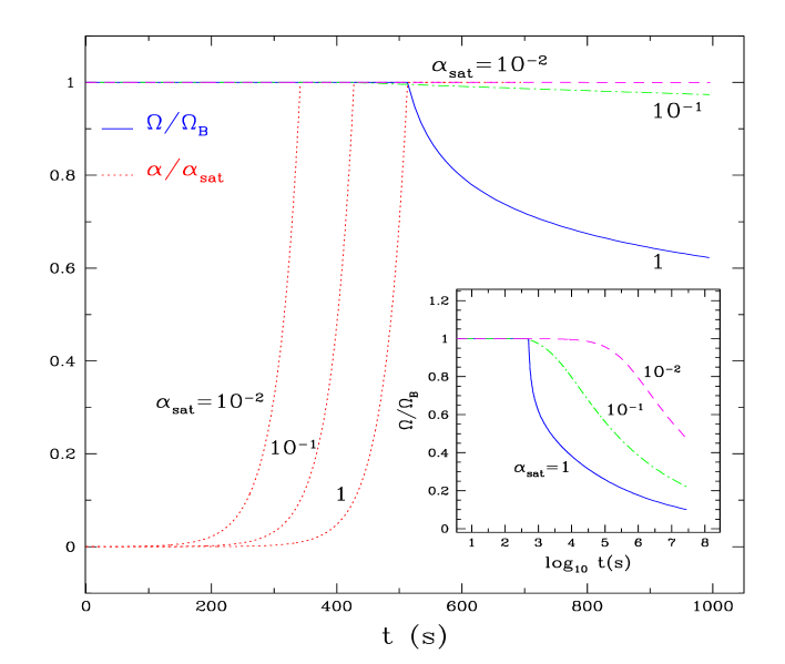
FIG. 1.: Time evolution of the mode amplitude (dotted lines) and of the star’s angular velocity (solid lines) normalized to the saturation value $\alpha_{\rm sat}$ and the break-up limit $\Omega_{{}_{\rm B}}$, respectively. Different curves refer to different values of the saturation amplitude. The small inset shows the decay of the star’s angular velocity on a logarithmic time scale.

Next, we consider the effect of an increasing mode amplitude on the kinematics of $r$-mode oscillations. For doing this we compute the equations of motion allowing the mode amplitude to vary as in Eq. (2) in the case before saturation. Fig. 2 shows the effect of a variable mode amplitude on the trajectories of two fiducial fluid elements following $r$-mode oscillations with $\ell=2$. We concentrate on two fluid elements which have the same initial longitude $\phi_{0}=0$ and latitude $\sim 50$ degrees, with the mode having an initial amplitude $\alpha_{0}=0.02$, which then saturates at $\alpha_{\rm sat}=0.1$. The initial positions are indicated with stars, while the positions at the end of each oscillation are indicated with filled squares. Note that in order to have a growth time which is larger but comparable with the oscillation period, we have artificially set $\Omega=5\Omega_{{}_{\rm B}}$ and the trajectories shown in Fig. 2 should therefore be considered only as indicative.

When compared with the corresponding trajectories shown in Fig. 1 of paper I, they show that the effect of an exponentially increasing mode amplitude is that of exponentially increasing the azimuthal and polar drifts between oscillations. As discussed in paper I when deriving the expression for the azimuthal drift [cf. Eq. (6) of paper I], one should expect secular effects to emerge every time that the velocity field at the position of the fluid element varies as it moves. This can happen either because the fluid velocity has a dependence on the position of the fluid element (as in the case of constant amplitude oscillations) or because the amplitude of the fluid velocity is changing (as during the growth of the instability). As a result, a mode amplitude which is exponentially growing in time will produce a secular motion, independently of whether the modes have reached nonlinear amplitudes.

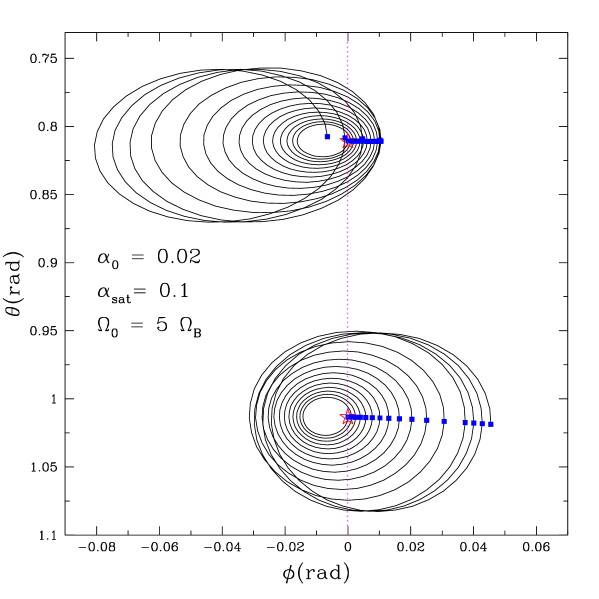
FIG. 2.: Projected trajectories $\theta(t)\sin\theta(t)\cos\phi(t)$, and $\phi(t)\sin\theta(t)\cos\phi(t)$ of two fiducial fluid elements as seen in the corotating frame. While the fluid elements are allowed to oscillate, the amplitude of the mode increases from an initial value $\alpha_{0}=0.02$ to a saturated one $\alpha_{\rm sat}=0.1$. The initial positions are indicated with stars, while the positions at the end of each period are indicated with filled squares. Note that we have set $\Omega=5\Omega_{{}_{\rm B}}$; this is to have a growth time which is larger but comparable with the oscillation period and to show schematically the effects of a increasing mode amplitude on the secular motions.

In the following Section, where we discuss the numerical evolution of the magnetic field as a result of the secular velocity field, it will be possible to distinguish the contribution to the field generation coming from the exponential growth phase of the mode from the one resulting from the secular drift at mode saturation.

B Evolution of the stellar magnetic field

We here present results from the solution of the induction equations as obtained with both the Lagrangian method [cf. Eq. (14) of paper I] and with the orbit-average method [cf. Eq. (16) of paper I] discussed in paper I. The computations have been performed for a number of different values of the saturation amplitudes, for modes with $\ell=2,3,4$, and with an initial dipolar magnetic field [cf. Eq. (8) of paper I].

From a numerical point of view, the Lagrangian and orbit-average approaches have a common strategy. Both of them, in fact, solve the equations of motion [cf. eqs. (3) of paper I] for a number of fiducial fluid elements suitably distributed on an isobaric surface of the star and calculated for several different mode numbers. In the Lagrangian approach, in particular, the new positions after each oscillation are used to reconstruct the strain tensor $S_{jk}=\partial{\tilde{x}}^{j}(t)/\partial{x}^{k}(t_{0})$ from which the new magnetic field components are computed. Conversely, in the numerically more expensive Eulerian approach, the secular polar and azimuthal velocities ${\tilde{v}}^{\hat{\theta}}$, ${\tilde{v}}^{\hat{\phi}}$ are computed after each oscillation period and their values transformed onto a finite difference grid corotating with the star, over which the induction equations are then solved. In this latter case, a second-order Lax-Wendroff evolution scheme is used to minimize artificial dissipative effects and accurately estimate the field growth rate.

     

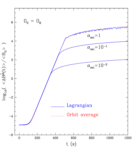
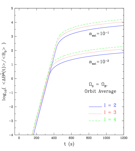
FIG. 3.: Growth of the logarithm of $\langle\Delta B^{\hat{\phi}}\rangle$ scaled to the initial poloidal field. The left panel refers to an $\ell=2$ mode and a number of different values of $\alpha_{\rm sat}$. The right panel shows the growth rate for different $\ell$ modes and two different saturation amplitudes. The underlying star has an initial angular velocity $\Omega_{0}$ equal to the break-up limit $\Omega_{{}_{B}}$, and $\langle B_{0}\rangle=10^{6}$ G. Note that in plotting the evolution of different mode numbers in the right panel we have assumed they all have the same growth time. This allows us to present them on a single plot but one should bear in mind the higher-order modes have considerably larger growth times [3].

Indicating by $\langle\Delta B^{\hat{i}}\rangle$ the $i$-th component of the volume average secular magnetic field, we show in Fig. 3 the time evolution of the averaged toroidal magnetic field normalized to the average initial magnetic field. The left panel of Fig. 3, in particular, shows the time evolution of the average toroidal field as computed with the Lagrangian approach (continuous lines) and with the orbit average approach (dotted lines). Different lines refer to different values of the saturation amplitude $\alpha_{\rm sat}$ and have been computed for an $\ell=2$ mode and a “fiducial” neutron star with mass $M=1.4{\rm M}_{\odot}$, radius $R=12.5$ km, and initial angular velocity $\Omega_{0}$ equal to the “break-up limit” $\Omega_{{}_{B}}\equiv(2/3)\sqrt{\pi G{\bar{\rho}}}$, with ${\bar{\rho}}=3M/(4\pi R^{3})$. The value of the initial toroidal field served only to set a lower limit to the vertical axis and was here set to be $10^{-6}\langle B_{0}\rangle$. Each line in the left panel shows an initial stage during which the toroidal field grows exponentially and a subsequent one during which the field has a growth which is a power-law of time. As mentioned in the previous Section, the two different regimes in the field growth reflect the fact that there are two regimes in which secular kinematic effects become apparent.

The first regime is related to the exponential growth of the mode amplitude and produces most of the new magnetic field. During this phase, the secular effects are extremely large [i.e. ${\cal O}(\alpha_{0}^{2}\exp(t))$] and the toroidal magnetic field is either produced or amplified by the wrapping of the poloidal magnetic field produced by the (mostly) toroidal secular velocity field. The amplification is so large that the toroidal magnetic field soon becomes comparable to and then larger than the seed poloidal field. Larger values of the saturation amplitude produce proportionally larger amplifications and these can be so dramatic in the case of $\alpha_{\rm sat}=1$, that the newly generated magnetic field at mode saturation has become about four orders of magnitude larger than any pre-existing magnetic field. Note that a magnetic configuration with strong toroidal magnetic fields is generally unstable and hoop magnetic stresses in the radial direction will tend to move magnetic field lines towards the poles [6]. Although the instability of this configuration might lead to a number of interesting astrophysical phenomena (see, for example, [7] where the buoyancy instability of this configuration is used for a $\gamma$-ray burst model), we will here assume that gas pressure gradients are always be able to counteract these hoop stresses.

The second regime is instead related to the saturated stage of the transition, during which the mode amplitude is constant in time. During this phase, the secular effects are much smaller [i.e. ${\cal O}(\alpha_{\rm sat}^{2}t)$] and so is the field growth rate, which is a power-law of time.

The left panel of Fig. 3 also gives a comparison between the Lagrangian and orbit-average methods. Despite the differences between the two approaches, the agreement is extremely good and deviations between the two appear only for the late-time, $\alpha_{\rm sat}=1$ growth rate, and at the beginning, when the growth rate is extremely small. This difference appears because of the difficulty of calculating the particle trajectories accurately for such large values of the mode amplitude and the inadequacy of the Lagrangian method in this regime.

     

FIG. 4.: Time evolution of $\langle\Delta B^{\hat{r}}\rangle$ (left panel) and of $\langle\Delta B^{\hat{\theta}}\rangle$ (right panel) scaled to the initial field strength. The calculation has been done with the orbit-average method for an $\ell=2$ mode and a saturation amplitude $\alpha_{\rm sat}=10^{-2}$.

The right panel of Fig. 3 shows the same quantity as the left one, but for different mode numbers and two different saturation amplitudes. Note that, in general, $r$ modes with different mode numbers saturate on different timescales, with the high-order modes having considerably longer growth times. However, in order to present them all in the same plot, we have assumed in the right panel of Fig. 3 that they all have the same timescale. Interestingly, higher mode numbers would, in principle, be more efficient in generating a toroidal magnetic field, and thus in converting the energy of the mode into magnetic energy, but modes with $\ell>2$ are also very unlikely to become unstable because of their longer growth times.

In Fig. 4 we show the corresponding evolution of the poloidal magnetic field components for an $\ell=2$ mode and a saturation amplitude $\alpha_{\rm sat}=10^{-2}$ as obtained through the orbit average method. Note that neither of the two poloidal magnetic field components shows a significant secular growth and that they both oscillate around the initial values. This is in agreement with Bragisnky’s dynamo model, whose velocity field has many analogies with the secular velocity field set up by the $r$ modes, and which predicts that the poloidal magnetic field should not be subject to a dynamo action and have a zero time average (see [8] for a complete discussion of Braginsky’s dynamo). Fig. 4 basically states that a large toroidal magnetic field will be the main outcome of the secular kinematic effects produced during the $r$-mode instability.

The numerical integration of the equations of motion and the calculation of the magnetic fields produced was usually stopped after 2000 s, corresponding to $\sim 10^{6}$ $r$-mode oscillations. At that stage and for our standard neutron star, the instability has already reached saturation and the toroidal field growth has entered a power-law growth phase which can be described analytically (cf. Fig. 5).

Fig. 5 synthesizes the results presented in the previous Figures and shows the time evolution of the total magnetic field $\langle\Delta B\rangle$ scaled to the initial magnetic field and over a timescale of one year. The left panel, in particular, refers to an $\ell=2$ mode, an initial angular velocity $\Omega_{0}=\Omega_{{}_{B}}$ and three different saturation amplitudes. The panel also presents a comparison between the fully numerical Lagrangian solution and the analytical one based on equations (26) and (27) of paper I. The agreement is remarkably good even for $\alpha_{\rm sat}\simeq 1$ when we expect the expansion procedures in powers of $\alpha$ to be rather poor.

     

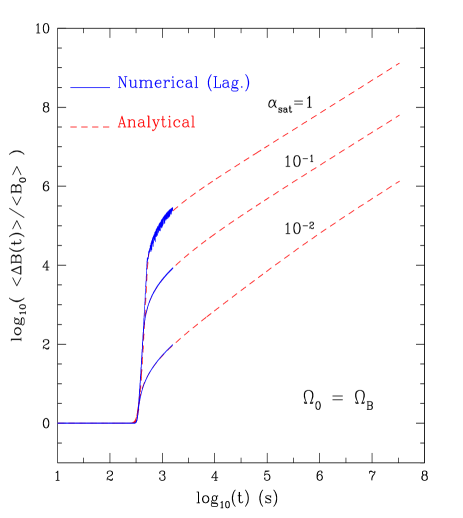
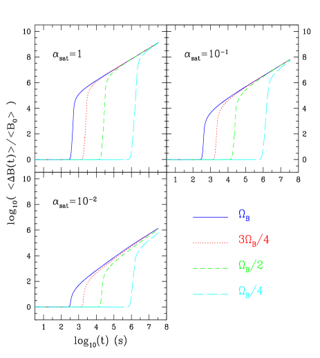
FIG. 5.: The left panel shows the long-time evolution of the logarithm of total magnetic field $\langle\Delta B\rangle$ scaled to the initial field for an $\ell=2$ mode and different saturation amplitudes. The star is set to have $\Omega_{0}=\Omega_{{}_{B}}$. The right panel is the same as the left one but shows the different evolutions resulting from values of the initial angular velocity $\Omega_{0}=\frac{1}{4}\Omega_{{}_{B}},\ \Omega_{0}=\frac{1}{2}\Omega_{{}_{B}},\ \Omega_{0}=\frac{3}{4}\Omega_{{}_{B}},\ \Omega_{0}=\Omega_{{}_{B}}$.

The right panel of Fig. 5 is the same as the left one but also shows the effect of a smaller initial angular velocity (i.e. $\Omega_{0}=\frac{1}{4}\Omega_{{}_{B}},\ \Omega_{0}=\frac{1}{2}\Omega_{{}_{B}},\ \Omega_{0}=\frac{3}{4}\Omega_{{}_{B}},\ \Omega_{0}=\Omega_{{}_{B}}$). Clearly, for stars rotating at slower angular velocities, the instability and the field growth set in at progressively later times. However, for any given saturation amplitude, the final magnetic field produced is rather insensitive of the rotation rate. This is because the magnetic field is generated mostly during the phase of exponential growth of the mode and as long as the star rotates sufficiently fast for the mode to grow unstable, the end result will remain roughly unchanged.

III Impact of Magnetic Fields

In paper I, as well as in the previous Sections of this paper, we have described how $r$-mode oscillations can produce secular drift velocity fields which, in a highly conducting plasma such as neutron star matter, can interact with pre-existing magnetic fields producing new ones. We have also discussed the set of equations that can be solved to calculate the magnitude of the newly generated magnetic fields and have solved them numerically to compute the values of the different magnetic field components produced for a number of different mode amplitudes and stellar angular velocities. We have not yet discussed the impact of these fields on the existence or growth of the $r$-mode oscillations. As mentioned in Section II, a fully self-consistent treatment is beyond the scope of this paper. However, important considerations can be made if we treat the $r$-mode instability and the generation of magnetic fields as evolving independently and with the magnetic field not “back-reacting” on the kinematic features of the $r$-mode oscillations. Under this simplifying hypothesis, it is possible to calculate the strength of the magnetic field necessary to prevent the amplification of the first $r$-mode oscillation, or damp the instability when this is free to develop. Both of these aspects are discussed in the following Sections IV and V.

IV Distortion of $r$ modes by the stellar magnetic field

As the magnetic field strength increases, the magnetic back-reaction forces generated by the $r$-mode motions of the fluid become larger and larger. As the magnetic field strength increases, the normal modes of the star corresponding to the zero-magnetic-field $r$ modes differ in character more and more from the zero-magnetic-field $r$ modes, taking on appreciable hydromagnetic and hydromagnetic-inertial properties. Eventually, the velocity perturbations corresponding to these normal modes are significantly different from the zero-magnetic-field $r$ modes to the point of preventing gravitational radiation from amplifying these distorted $r$-mode oscillations.

Since the normal modes of the star are global in character, the effects of a magnetic field cannot be analyzed fully by a local analysis, such as can be done by making a local comparison of forces. In contrast, a mode-energy approach takes into account the global properties of the modes and magnetic field and this is what we will consider in the following. During an oscillation the energy in the magnetic field will rise and fall. If there is not enough energy in the mode to supply the maximum magnetic energy increase required to complete an oscillation, a “full” $r$-mode oscillation will not occur (some other, smaller scale pulsations might still occur). Stated differently, if the magnetic field exceeds a critical value, $B_{\rm crit,p}$, the magnetic stress that builds up during an oscillation will be so large that it will halt the fluid motion involved in the oscillation, i.e. the fluid momentum density will be brought to zero. The condition that defines $B_{\rm crit,p}$ is therefore

$$\delta E_{{}_{\rm M}}=\widetilde{E}\ ,$$ (5)

where $\widetilde{E}$ the energy in the mode as measured in the corotating frame of the equilibrium star

$$\widetilde{E}=\frac{1}{2}\frac{\alpha^{2}\Omega^{2}}{R^{2}}\int^{R}_{0}\rho\,r^{6}dr\simeq 8.2\times 10^{-3}\alpha^{2}M\Omega^{2}R^{2}\ ,$$ (6)

and $\delta E_{{}_{\rm M}}$ is the change in magnetic energy density

$$\delta E_{{}_{\rm M}}\equiv\frac{1}{8\pi}\int_{V_{\infty}}\delta B^{2}{\;d^{3}{\bf x}}\ ,$$ (7)

with $\delta B^{2}=(\delta B^{\hat{p}})^{2}+(\delta B^{\hat{\phi}})^{2}$. Note that the fractional change in the mode energy produced by gravitational wave emission during a single oscillation period is $4\pi/\omega|\tau_{{}_{\rm GW}}|$. This is always $\ll 1$ and therefore can be neglected in this comparison.

The expression for $\delta E_{{}_{\rm M}}$ varies according to whether the neutron star core is composed of a normal neutron fluid (N) or is superconducting (SC). More particularly, we denote as $\delta E^{\rm N}_{{}_{\rm M}}$ and $B^{\rm N}_{\rm crit,p}$ the magnetic energy and the critical, volume averaged, magnetic field for a normal core. Similarly, we denote as $\delta E^{{}^{\rm SC}}_{{}_{\rm M}}$ and $B^{{}^{\rm SC}}_{\rm crit,p}$ the corresponding quantities for a superconducting core. The two cases will be considered separately below.

A When the stellar core is normal

The induction equation can be integrated in time to estimate the variations in the magnetic field produced by the perturbation velocity field as

$$\delta B^{\hat{\theta}}\simeq B^{\hat{\phi}}_{0}\int{\dot{\theta}}(t^{\prime})dt^{\prime}\simeq B^{\hat{\phi}}_{0}\int\frac{\delta v(t^{\prime})}{r}dt^{\prime}\simeq\delta B^{\hat{p}}\ ,$$ (8)

$$\delta B^{\hat{\phi}}\simeq B^{\hat{\theta}}_{0}\int{\dot{\phi}}(t^{\prime})dt^{\prime}\simeq B^{\hat{\theta}}_{0}\int\frac{\delta v(t^{\prime})}{r}dt^{\prime}\ ,$$ (9)

where we have set ${\dot{\theta}}\simeq{\dot{\phi}}\simeq\delta v/r$. Because of the periodic variation of the magnetic energy during an oscillation, expression (7) should be averaged over half of an oscillation period, so that the magnetic energy produced is

$$\delta E^{\rm N}_{{}_{\rm M}}=\left(\frac{9\pi}{32}\right)\frac{1}{\Omega^{2}}\int_{V_{*}}\left[B_{0}\frac{\delta v}{r}\right]^{2}{\;d^{3}{\bf x}}\ .$$ (10)

In deriving (10) we have not included contributions to $\delta E_{{}_{\rm M}}$ from changes in the magnetic field outside the star which are heavily suppressed by the high electric conductivity of the crust. Also, we have written the time average of the velocity perturbation as

$$\int^{P/2}_{0}\delta v(t^{\prime})dt^{\prime}\simeq\left(\frac{3\pi}{2}\right)\frac{\delta v}{\Omega}\ .$$ (11)

Note that both energies (6) and (10) depend quadratically on the velocity perturbation $\delta v$ and therefore on $\alpha$. As a result, the critical fields are not not sensitive to the amplitude development of the mode. The volume integral can be easily performed after assuming an initial dipolar magnetic field: $B_{0}=B_{\rm d}(R/r)^{3}\Psi(\theta)$, where $\Psi(\theta)\equiv 4\cos^{2}\theta+\sin^{2}\theta$. Indicating with $|{\mathbf{Y}}^{B}_{22}(\theta,\phi)|$ the modulus of the vector spherical harmonic, the magnetic energy produced over half of a period is then

$$\delta E^{{}^{\rm N}}_{{}_{\rm M}}=\left(\frac{9\pi}{32}\right)B^{2}_{\rm d}R^{4}\alpha^{2}\int^{2\pi}_{0}d\phi\int^{\pi}_{0}|{\mathbf{Y}}^{B}_{22}(\theta,\phi)|\Psi(\theta)\sin\theta d\theta\int^{R}_{pR}r^{-2}dr=\left[\frac{3\pi(1-p)}{32p}\right]\Lambda\alpha^{2}B^{2}_{\rm d}R^{3}\ ,$$ (12)

where all of the angular dependence is contained in $\Lambda$

$$\Lambda\equiv\int^{2\pi}_{0}d\phi\int^{\pi}_{0}|{\mathbf{Y}}^{B}_{22}(\theta,\phi)|\Psi(\theta)\sin\theta d\theta={\mathcal{O}}(1)\ .$$ (13)

It is worth noticing that we can here neglect the distortion of the magnetic field near the crust-core boundary during an $r$-mode oscillation. The reason for this is that, on the timescales relevant for the $r$ modes and regardless of whether the core is superconducting, the magnetic field lines (and flux tubes) are pinned in place at the crust-core boundary by the high conductivity of the crust.

Using (12) with $p=0.5$ and (13), we can now write the condition for $r$-mode prevention (5) in terms of a critical field given by

$$B^{{}^{\rm N}}_{\rm crit,p}\simeq 2.5\times 10^{16}\left(\frac{\Omega}{\Omega^{*}_{B}}\right)\left(M_{1.4}\right)^{1/2}\left(R_{12.5}\right)^{-1/2}\ {\rm G}\ ,$$ (14)

where $M_{1.4}\equiv M/1.4\,M_{\odot}$, $R_{12.5}\equiv R/12.5\,{\rm km}$, and $\Omega^{*}_{B}\equiv 5.62\times 10^{3}$ rad s^-1.

B When the stellar core is superconducting

When, as a result of the star’s cooling, the core temperature falls below a critical value, $T_{c}\sim 3\times 10^{9}$ K, the core is expected to become a Type II superconductor [10]. In such a superconducting core, the magnetic field is confined to flux tubes and the total energy of the flux tubes can be computed in terms of the total number $N$ of flux tubes in the core and of the mean total energy of a flux tube

$$\langle e\rangle=\frac{\phi_{0}}{8\pi}\langle H_{f}\ell_{f}\rangle\ ,$$ (15)

with $\ell_{f}$ being the average length of a flux tube, $H_{f}$ the magnetic field inside it and $\phi_{0}=hc/(2e)\simeq 2\times 10^{-7}$ G cm² the flux quantum. The total magnetic energy of the flux tubes of the unperturbed star is then

$$E^{{}^{\rm SC}}_{{}_{\rm M}}=\frac{\phi_{\rm tot}}{8\pi}\langle H_{f}\ell_{f}\rangle\ ,$$ (16)

where $\phi_{\rm tot}\approx\pi R^{2}B_{\rm d}$ is the total magnetic flux. The $r$-mode oscillations will shear and stretch the flux tubes, increasing their length by ${\delta\ell}$, and thus changing their energy content by an amount $\delta E^{{}^{\rm SC}}_{{}_{\rm M}}=({\phi_{\rm tot}}/{8\pi})H_{f}\delta\ell_{f}$ over half a period. Estimating the volume-averaged variation in the flux tube length as

$$\delta\ell\simeq\frac{9\pi^{2}}{56}\alpha^{2}R\ ,$$ (17)

we then obtain

$$\delta E^{{}^{\rm SC}}_{{}_{\rm M}}\simeq\frac{27\pi^{2}}{448}\alpha^{2}H_{f}B_{\rm d}R^{3}\simeq 4.5\times 10^{34}\alpha^{2}\left(\frac{H_{{}_{C1}}}{4.4\times 10^{15}}\right)B_{\rm d}R^{3}_{12.5}\ {\rm ergs}\ ,$$ (18)

where we have taken $H_{f}\approx H_{{}_{C1}}$, the lower critical field [9].

Note that expression (18) is only valid when the spacing between the flux tubes is much larger than the London penetration length, i.e. for $\langle B\rangle\ll H_{{}_{C1}}$. However, as $\langle B\rangle$ rises above $H_{{}_{C1}}$ and tends to the upper critical field $H_{{}_{C2}}\approx 10^{17}$ G, $H_{f}$ also rises and tends to $H_{{}_{C2}}$, with the flux tubes crowding one another. When $\langle B\rangle=H_{{}_{C2}}$, the normal cores of the flux tubes touch, the superconducting state is destroyed [9] and the variation in the magnetic energy is then again given by expression (12). Combining (18) with (12), we can now write the condition for $r$-mode prevention in terms of the critical field for a superconducting core

$$B^{{}^{\rm SC}}_{\rm crit,p}\simeq 9.7\times 10^{16}\left(\frac{\Omega}{\Omega^{*}_{B}}\right)^{2}M_{1.4}\left(R_{12.5}\right)^{-1}\left(\frac{H_{{}_{C1}}}{10^{16}\ {\rm G}}\right)^{-1}\ {\rm G}\ .$$ (19)

As for the critical field for a normal core, expression (19) is insensitive to the values of the mode saturation amplitude, underlining that if $B_{0}>B_{\rm crit,p}$ even very small amplitude fluctuations of $r$-mode character cannot occur. On the other hand, the critical fields are sensitive to the star’s spin rate; in particular, if $\Omega$ is $\approx\Omega^{*}_{B}$, the magnetic field needed to prevent oscillation of the $\ell=2$ mode is $\sim 10^{16}\,{\rm G}$ and hence $B_{{\rm crit},p}\sim B^{N}_{{\rm crit},p}$, whether or not the core is superconducting. If instead $\Omega\ll\Omega^{*}_{B}$, then $B_{{\rm crit},p}^{SC}\approx 10^{13}\,(\Omega/0.01\,\Omega_{B}^{*})^{2}H_{C1,16}^{-1}M_{1.4}R_{12.5}^{-1}\,$G, where $H_{C1,16}\equiv H_{C1}/10^{16}\,{\rm G}$.

The critical fields (14) and (19) are several orders of magnitude larger than the typical magnetic fields of young neutron stars that observations indicate to be in the range $10^{11}-10^{13}$ G. This suggests that the distortion of the first $r$-mode oscillations by magnetic fields is rather unlikely and that the $r$-mode instability in newly born neutron stars (or any compact object with analogous properties) is, in general, free to develop. The onset of the instability, however, will also lead to the production of very intense magnetic fields which could ultimately lead to the damping of the oscillations, as discussed below.

V Damping of $r$ modes by the stellar magnetic field

The damping of oscillations by the growing magnetic field reflects the question of whether the energy required to continue the oscillation for the next time step $\Delta t$ exceeds the energy that can be pumped into the mode in the time $\Delta t$ by the emission of gravitational radiation.

A When the stellar core is normal

A critical point in the balance between the energy spent in producing magnetic field and the energy in the mode provided by the emission of gravitational waves is reached when the two rates are equal

$$\frac{dE_{{}_{\rm M}}}{dt}=\left(\frac{d{\widetilde{E}}}{dt}\right)_{{}_{\rm GW}}\ ,$$ (20)

where

$$\left({d\widetilde{E}\over dt}\right)_{{}_{\rm GW}}=-{32\pi G\over c^{7}}\left[{4\over 3(5)!!}\right]^{2}\frac{\alpha^{2}\Omega^{4}\omega^{4}}{R^{2}}\left(\int_{0}^{R}\rho\,r^{6}dr\right)^{2}\ ,$$ (21)

is the rate of energy transferred to an $\ell=2$ mode [3]. After the equality (20) is reached, ${dE_{{}_{\rm M}}}/{dt}>(d{\widetilde{E}}/{dt})_{{}_{\rm GW}}$. The reason for this is that the toroidal magnetic field, and hence ${dE_{{}_{\rm M}}}/{dt}$, will continue to grow whereas $(d{\widetilde{E}}/{dt})_{{}_{\rm GW}}$ remains the same or decreases as gravitational radiation causes the star to spin down. The only source of energy to feed $E_{{}_{\rm M}}$ is thus the energy ${\widetilde{E}}$ of the mode which damps on a timescale

$$\tau_{{}_{\rm M}}=\frac{\widetilde{E}}{({dE_{{}_{\rm M}}}/{dt})}\ .$$ (22)

A measure of the relative importance of the two energy rates can be obtained through considering their ratio

$$g(t)\equiv\frac{{dE_{{}_{\rm M}}}/{dt}}{(d{\widetilde{E}}/{dt})_{{}_{\rm GW}}}\ ,$$ (23)

where, in the case of normal core, the rate of production of magnetic energy takes the form

$$\frac{dE^{{}^{\rm N}}_{m}(t)}{dt}=\left[\frac{4(1-p)}{9\pi p}\right]B^{2}_{{}_{S}}R^{3}\Lambda^{\prime}\alpha^{2}(t)\Omega(t)\int^{t}_{0}\alpha^{2}(t^{\prime})\Omega(t^{\prime})dt^{\prime}\ ,$$ (24)

with now $\Lambda^{\prime}\equiv\int^{2\pi}_{0}d\phi\int^{\pi}_{0}(\kappa_{2}(\theta))^{2}|{\mathbf{Y}}^{B}_{22}(\theta,\phi)|\Psi(\theta)\sin\theta d\theta$, which is again ${\mathcal{O}}(1)$.

Fig. 6 shows the numerical computation of the ratio (23) for a “fiducial” neutron star initially rotating at the break-up limit $\Omega^{*}_{B}$. The rate of energy loss to gravitational radiation has been computed for an $\ell=2$ mode and a polytropic equation of state with $\Gamma=2$. The left panel shows the time evolution of $g(t)$ for saturation amplitudes $\alpha_{\rm sat}=0.1$ and four different values of the initial magnetic field $\langle B_{0}\rangle$ which are indicated with different types of thick lines. The right panel is the same as the left one except for having $\alpha_{\rm sat}=1$. For each curve in Fig. 6 it is straightforward to distinguish the initial phase of exponential growth of the magnetic field (and of the magnetic energy production rate) from the subsequent phase of power-law growth. It also appears evident that, for a given saturation amplitude, different values of $\langle B_{0}\rangle$ have only the effect of moving the curves in the vertical direction: the smaller the initial field, the longer it will take to reach a sufficiently strong magnetic field necessary for suppression.

As discussed in paper I, we expect the drift of fluid elements given by the velocity field ${\mathbf{v}}_{\rm d}$ [cf. Eq. (7) of paper I] to be qualitatively correct to ${\cal O}(\alpha^{2})$. However, within our approach we cannot exclude the possibility that the actual drift velocity is smaller (or larger) than the estimated one. To assess the variations brought about by a smaller secular velocity field, we use the thin lines in Fig. 6 that are near to the thick lines of the same type to show the magnetic field evolution which has been calculated with the secular velocity field being one tenth of that computed in paper I. Because of the exponential growth in the mode amplitude and in the toroidal magnetic field, the overall differences produced are rather small.

 

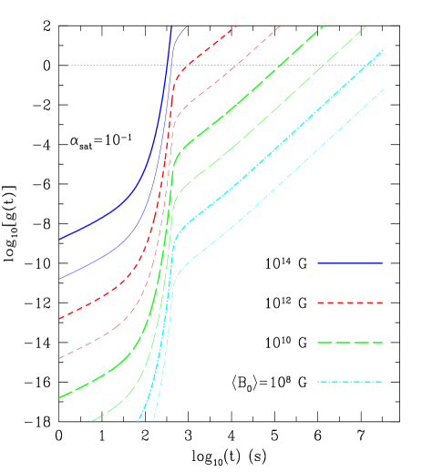
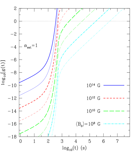
FIG. 6.: Time evolution of the ratio $g(t)$. The calculation refers to our “fiducial” neutron star initially rotating at the break-up limit $\Omega^{*}_{B}$. The left and right panels show the evolution for different values of the saturation amplitude. Lines of different type refer to different values of the initial magnetic field $\langle B_{0}\rangle$. Nearby thick and thin lines of the same type are used to compare the magnetic field evolution produced by the secular velocity field calculated in paper I [cf. Eq. (7) of paper I] and a velocity field which is just a tenth of it.

When read in terms of the times at which suppression of the oscillations begins, Fig. 6 indicates that for an initial magnetic field $\langle B_{0}\rangle=10^{10}-10^{12}$ G, the instability starts to be suppressed after a time between 2 days and 15 minutes for a saturation amplitude $\alpha_{\rm sat}=0.1$ (see also Table I). When this happens the total magnetic fields produced are in the range $10^{14}-10^{15}$ G. The condition for oscillation suppression (20) can also be used to calculate $\Omega_{\rm crit}$: the critical spin rate above which $r$ modes are excited and below which they are damped. Values of the critical angular velocity for a normal core normalized to the break-up angular velocity $\Omega^{*}_{B}$ are indicated in Table I. The Table reports the critical spin rates as a function of the initial magnetic field strengths for a number of different saturation amplitudes. For each pair of these parameters, we also indicate in brackets the time (in seconds) $t_{\rm crit}$ at which the condition (20) is reached. As we will discuss in Section VI, the knowledge of the critical angular velocity is in fact very important as it provides the final (and maximum) gravitational wave frequency at which the last gravitational radiation is emitted. Together with the initial star’s spin frequency, the maximum frequency determines the domain over which a signal-to-noise ratio can be calculated [cf. Eq. (30)].

It is worth underlining that even when the $r$-mode instability is rapidly suppressed by generation of intense magnetic fields, there is sufficient time for the star to loose a good fraction of its rotational energy to gravitational waves. This is because the loss-rate of angular momentum to gravitational waves is a steep function of the star’s angular velocity [cf. Eq. (4)] and is large mostly soon after the amplitude saturation. Therefore, for initial magnetic fields of the order of $10^{10}$ G, most of the astrophysical considerations about the importance of the $r$-mode instability in spinning down newly-born neutron stars [11] are basically unchanged. $\Omega^{{}^{\rm N}}_{\rm crit}/\Omega^{*}_{B},\ \ (t_{\rm crit}$ in s) $\langle B_{0}\rangle=10^{8}\$G $\langle B_{0}\rangle=10^{10}\$G $\langle B_{0}\rangle=10^{12}\$G $\langle B_{0}\rangle=10^{14}\$G $\alpha_{\rm sat}=1.0~{}~{}~{}$ 0.318   ($2.90\times 10^{5}$) 0.467   ($3.34\times 10^{3}$) 0.948   ($5.24\times 10^{2}$) 0.999   ($3.52\times 10^{2}$) $\alpha_{\rm sat}=10^{-1}$ – 0.535   ($1.37\times 10^{5}$) 0.975   ($9.75\times 10^{2}$) 0.999   ($3.23\times 10^{2}$) $\alpha_{\rm sat}=10^{-2}$ – – 0.974   ($5.62\times 10^{4}$) 0.999   ($3.23\times 10^{2}$)
TABLE I.: Normalized critical angular velocities [i.e. final values of the star’s angular velocity when $g(t)=1$, normalized to the initial break-up angular velocity $\Omega^{*}_{B}$] for different values of the magnetic field $\langle B_{0}\rangle$ and saturation amplitude $\alpha_{\rm sat}$. Values not reported refer to times longer than one year, for which the instability is suppressed by viscosity rather than by the production of magnetic field. The numbers in brackets indicate the time (in seconds) after which the condition for suppression is reached.

B When the stellar core is superconducting

In the case of a superconducting core, the calculation of the damping of the $r$ mode oscillations is slightly more complicated (and uncertain) because additional considerations need to be made about the time variations of the total magnetic flux $\phi_{\rm tot}$ and about the magnetic field components that contribute mostly to the flux. Once $B^{\hat{\phi}}$ exceeds $B^{\hat{p}}$, the magnetic energy rate can be expressed as

$$\frac{dE^{{}^{\rm SC}}_{{}_{\rm M}}(t)}{dt}\simeq\frac{\kappa_{2}(\theta)}{60}H_{{}_{C1}}B^{\hat{p}}R^{3}\alpha^{2}(t)\Omega(t)\ .$$ (25)

Hence, for a superconducting core, the actual critical spin rate is likely to be

$$\Omega^{{}^{\rm SC}}_{\rm crit}\simeq 0.7\,\Omega_{B}^{*}\,\left(\frac{B^{\hat{p}}}{10^{12}{\rm G}}\right)^{1/7}\left(\frac{H_{f}}{10^{16}{\rm G}}\right)^{1/7}M_{1.4}^{-2/7}R_{12.5}^{-3/7}\ ,$$ (26)

which is again independent of the mode amplitude.

VI Gravitational wave detectability

The relevance of the gravitational radiation emitted by $r$-modes oscillations has been investigated by a number of authors who have considered them both as single sources [3, 12, 13] and as a cosmological population producing a stochastic background [14]. Their estimates indicate that sufficiently close sources might be detectable by LIGO and VIRGO when they reach their “enhanced” level of sensitivity or that two nearby interferometers with “advanced” sensitivities might be used for the detection.

Using the results obtained in the previous Section and bearing in mind the simplifying assumptions under which they have been derived, we now re-evaluate the possibility of detecting gravitational waves from $r$ modes in magnetic neutron stars. All of the results discussed below refer to a “fiducial” neutron star with a normal core. For an $\ell=2$ mode, the rate of angular momentum loss due to the emission of gravitational waves can be written as [3]

$${dJ_{c}\over dt}=\frac{D^{2}}{2}\omega\langle\langle h_{+}^{2}+h_{\times}^{2}\rangle\rangle\ ,$$ (27)

where $h_{+}$ and $h_{\times}$ are the strain amplitudes of the two polarizations of gravitational waves, $D$ is the distance to the source, and $\langle\langle\ldots\rangle\rangle$ denotes the average over the orientation of the source and its location on the sky. Here $J_{c}=-3\tilde{J}MR^{2}\Omega_{s}\alpha^{2}$ is the canonical angular momentum [15] (see also [3]) and $\tilde{J}=\int_{0}^{R}\rho\,r^{6}dr/(MR^{4})$.

Following [3], the averaged gravitational wave amplitude is then given by

$$h(t)=\sqrt{\frac{1}{10}\langle\langle h_{+}^{2}+h_{\times}^{2}\rangle\rangle}=\frac{256}{135}\sqrt{\frac{\pi}{30}}\frac{GM}{c^{5}}\frac{\alpha\Omega^{3}R^{3}}{D}\tilde{J}\ ,$$ (28)

and its time evolution for a “fiducial” neutron star placed at 20 Mpc is shown in Fig. 7. The left panel, in particular, shows evolutionary tracks for a number of different initial values of the magnetic field and a saturation amplitude $\alpha_{\rm sat}=1$. The tracks terminate when $g(t)=1$, which is marked with an open symbol (different symbols refer to different initial magnetic fields). The right panel, on the other hand, refers to an initial magnetic field $\langle B_{0}\rangle=10^{10}$ G and shows the effect of different saturation amplitudes on the reaching of a magnetic energy production rate sufficient to suppress the instability (which occurs at the point marked with filled squares). Taking a saturation amplitude $\alpha_{\rm sat}=0.1$, one sees that the emission of gravitational waves would start being suppressed after about 20 days.

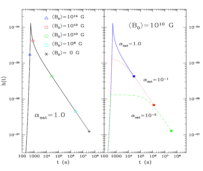
FIG. 7.: Time evolution of the averaged gravitational wave amplitude. The left panel is for a saturation amplitude $\alpha_{\rm sat}=1$ and shows the different behaviour with different initial values of the magnetic field. The evolutionary tracks terminate when $g(t)=1$ and different final points are marked with different open symbols. The right panel refers to an initial field of $\langle B_{0}\rangle=10^{12}$ G and shows the influence of the saturation amplitude on the evolution of the wave amplitude. A filled square indicates the time at which $g(t)=1$.

A more useful quantity for discussing the detectability of the gravitational waves emitted is the characteristic amplitude $h_{c}$, defined as

$$h_{c}(f)\equiv h(t)\sqrt{f^{2}\bigg{|}\frac{dt}{df}\bigg{|}}\ ,$$ (29)

where $f$ is the gravitational wave frequency and $f=\omega/(2\pi)=2\Omega/(3\pi)$ for a $\ell=2$ mode.

In Fig. 8 we show the frequency evolution of the characteristic amplitude for a magnetic neutron star located at 20 Mpc and with a saturation amplitude $\alpha_{\rm sat}=1$. As in Fig. 7, different symbols mark the frequency at which $g(t)=1$ for different values of the initial magnetic field. The frequency evolutionary track should be compared to the expected root-mean-square strain noise $h_{\rm rms}$ curves, indicated with dashed lines Fig. 8 and referring to the LIGO “first interferometers” (LIGO I), to the “enhanced interferometers” (LIGO II), and to the “advanced interferometers” (LIGO III). Analytic expressions for the expected $h_{\rm rms}$ have been presented in [3].

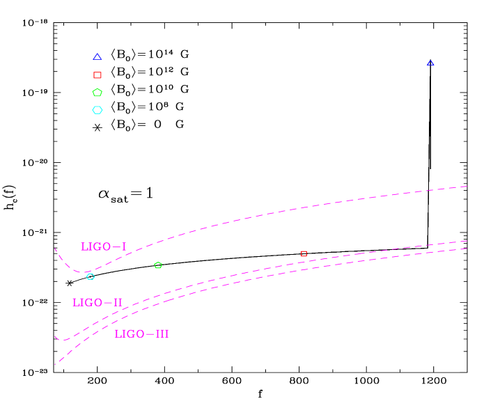
FIG. 8.: Frequency evolution for the characteristic amplitude for a magnetic neutron star located at 20 Mpc and with a saturation amplitude $\alpha_{\rm sat}=1$. As in Fig. 7, different symbols mark the frequency at which $g(t)=1$ for different values of the initial magnetic field. The three dashed lines show the expected $h_{\rm rms}$ for the three stages of development of the LIGO interferometers. Note that the spike in $h_{c}$ is the result of a vanishing $df/dt$ at the onset of the instability and does not contribute significantly to the SNR.

The characteristic amplitude also allows a direct calculation of the signal-to-noise ratio (SNR) for a single source at a distance $D$. Using matched filtering techniques, the SNR can be written as [3]

$$\left({S\over N}\right)^{2}=2\int^{f_{\rm max}}_{f_{\rm min}}{df\over f}\left({h_{c}\over h_{\rm rms}}\right)^{2}\ ,$$ (30)

where, for a strain noise with power spectrum $S_{h}(f)$, $h_{\rm rms}\equiv\sqrt{fS_{h}(f)}$. The integral in (30) is computed between the minimum frequency $f_{\rm min}=2\Omega_{0}/(3\pi)$ and the maximum frequency $f_{\rm max}=2\Omega_{\rm crit}/(3\pi)$ at which the gravitational radiation is emitted, but is largely dominated by the amplitude-saturated part of the evolution. As a consequence, it is strongly influenced by the angular velocity at which the mode is suppressed $\Omega_{\rm crit}$ and, as discussed in the previous Section, on the initial strength of the magnetic field.

In Table II we report the results of the calculation of signal-to-noise ratios obtained through the evolutionary models discussed in the previous Sections. The SNR are given for $\alpha_{\rm sat}=1$, ($\alpha_{\rm sat}=10^{-1}$) and different values of the initial magnetic field. For a zero initial magnetic field and $\alpha_{\rm sat}=1$, we recover the results obtained by [3]

$S/N:\alpha_{\rm sat}=1$	$\langle B_{0}\rangle=0\$G	$\langle B_{0}\rangle=10^{8}\$G	$\langle B_{0}\rangle=10^{10}\$G	$\langle B_{0}\rangle=10^{12}\$G	$\langle B_{0}\rangle=10^{14}\$G
$(\alpha_{\rm sat}=10^{-1})$
LIGO-I	1.2 (0.7)	0.8 (—)	0.4 (0.4)	0.1 (0.1)	$<0.01$
LIGO-II	7.6 (4.1)	4.8 (4.1)	2.2 (2.1)	0.8 (0.6)	$<0.01$
LIGO-III	10.6 (5.4)	6.4 (5.4)	2.9 (2.7)	1.1 (0.8)	$<0.01$

TABLE II.: Signal-to-Noise ratios for different values of the saturation amplitude $\alpha_{\rm sat}$ and of the initial magnetic field $\langle B_{0}\rangle$. The values referring to a zero initial magnetic field coincide with those calculated by [3]. As for Table I, the values not reported refer to times longer than one year.

Note that the presence of a relatively weak initial magnetic field (i.e. $\langle B_{0}\rangle=10^{8}$ G) does not significantly change the SNR as compared to an neutron star with zero magnetic field. However, this is not the case when the initial magnetic field is taken to be stronger and, in particular, for an initial $\langle B_{0}\rangle=10^{12}$ G, the SNR is such that even LIGO-III would only be able to detect it if $\alpha_{\rm sat}$ is ${\cal O}(1)$. Overall our results indicate therefore that the development of the $r$-mode instability in a magnetic neutron star could significantly reduce the expectations of detection of gravitational waves from $r$-mode oscillations.

VII Conclusions

We have computed numerically the growth of the magnetic field generated by the secular kinematic effects emerging during the evolution of the $r$-mode instability. We have treated the magnetic field growth as a kinematic dynamo problem, thus neglecting any back-reaction of the magnetic field on the forces driving the velocity field. The toroidal magnetic field computed in this way exhibits an exponential growth which is a direct consequence of the exponential development of the $r$-mode instability. During this stage of the growth, the toroidal field can become extremely large and, in the case of a saturation amplitude of order unity, it can grow to be four orders of magnitude larger than the seed poloidal field. At mode saturation and thereafter, the field growth rate is smaller but nonzero, thus still contributing significantly to the production of very intense magnetic fields.

Although we have neglected the back-reaction of the magnetic field on the kinematics of the $r$-mode oscillations, we can estimate the strength of the magnetic fields that would either prevent the onset of the $r$-mode instability or damp it when this is allowed to grow. Our estimates indicate that the critical initial magnetic field which would suppress even the first $r$-mode oscillation is $\langle B_{0}\rangle_{\rm crit}\sim 10^{16}$ G and this is basically independent of whether the core is superconducting or not. Such a magnetic field is two orders of magnitude larger than those usually associated with young neutron stars and it is therefore likely that most newly born neutron stars will have an initial magnetic field which is sufficiently weak for the instability to be triggered. However, depending on the strength of the initial magnetic field and on the mode amplitude at saturation, an $r$-mode instability which is initially free to develop could be subsequently damped by the generation of magnetic fields on timescales much shorter than the ones set by viscous effects. As an example, with an initial magnetic field strength $\langle B_{0}\rangle=10^{10}$ G and a normal stellar core, we find that the instability would be suppressed in less than four hours for a saturation amplitude $\alpha_{\rm sat}=1$ and in less than ten days for $\alpha_{\rm sat}=0.1$.

An important point to stress is that even in the case the $r$-mode instability is rapidly suppressed by the coupling of the mass-currents with magnetic fields, the star will have had sufficient time to loose a good fraction of its rotational energy to gravitational waves. This is because the loss-rate of angular momentum to gravitational waves is a steep function of the star’s angular velocity and is therefore most efficient only in the very initial stages of the instability. As a result, for realistic values of the initial magnetic field, most of the astrophysical considerations about the importance of the $r$-mode instability in spinning down newly-born neutron stars remain basically valid.

The validity of our scenario could be verified in a number of ways. As discussed in the previous Section, the larger the initial magnetic field, the sooner the condition for mode damping will be reached. We could therefore expect a positive correlation of the stellar spin rate at about one year and the initial poloidal magnetic field of the neutron star. For the same reason, we could expect an anti-correlation between the stellar spin rate and the toroidal magnetic field at about one year. Our results also have a direct impact on the gravitational wave detectability of $r$ modes from unstable neutron stars. Since the SNR for the detection of gravitational waves from $r$-mode oscillations depends sensitively on the star’s spin frequency at mode suppression, and the latter is determined by the mode amplitude at saturation and the initial magnetic field, we have found that the SNR could be significantly above unity only if the initial magnetic field is below $10^{12}$ G. Moreover, because of the quantitative difference in the mode damping in the case of a superconducting stellar core, the determination of the critical frequency could be used to infer a signature of the onset of proton superconductivity in the core.

Finally, we note that some fundamental issues remain unresolved. A most outstanding one is whether the magnetic field will distort the $r$-mode velocity field in such a fine-tuned way so as to cancel the fluid drift before it suppresses the oscillation. As discussed in [1], considerations of the energy densities in play suggest that this is rather unlikely, but a more detailed analysis of this would certainly provide important information about the evolution of the $r$-mode instability in magnetic neutron stars.

- [1] L. Rezzolla, F. K. Lamb, and S. L. Shapiro, 1999, Astrophys. J. 531, L141 (2000).
- [2] L. Rezzolla, F. K. Lamb, D. Marković, and S. L. Shapiro, Phys. Rev. D, (2001), paper I.
- [3] B. J. Owen, L. Lindblom, C. Cutler, B. F. Schutz, A. Vecchio, and N. Andersson, Phys. Rev. D 58, 084020 (1998).
- [4] L. Lindblom, B. J. Owen, and S. M. Morsink, Phys. Rev. Lett. 80, 4843 (1998).
- [5] N. Andersson, K. D. Kokkotas, and B. F. Schutz, 1999, Astrophys. J. 510, 846
- [6] D. Biskamp, Nonlinear Magnetohydrodynamics, Cambridge Univ. Press, Cambridge, Great Britain (1993).
- [7] H. C. Spruit, Astron. and Astrophys. 341, L1 (1999).
- [8] H. K. Moffatt, Magnetic Field Generation in Electrically Conducting Fluids, Cambridge Univ. Press, Cambridge, Great Britain, pp.179-196 (1978).
- [9] P. G. de Gennes, Superconductivity of Metals and Alloys, New York, Benjamin (1966)
- [10] F. K. Lamb, in Frontiers of Stellar Evolution, ed. D. L. Lambert, Astronomical Society of the Pacific, pp. 299-388 (1991)
- [11] N. Andersson, and K. D. Kokkotas, Int. Journ. of Mod. Phys. D, in press (2000).
- [12] P. R. Brady, and T. Creighton, Phys.Rev. D 61, 082001 (2000).
- [13] C. L. Fryer, D. E. Holz, and S. A. Hughes, preprint astro-ph/0106113 (2001).
- [14] V. Ferrari, S. Matarrese, and R. Schneider, Mon. Not. R. Astr. Soc. 303, 258 (1999).
- [15] J. L. Friedman and B. F. Schutz, Astrophys. J. 222, 281 (1978)