Properties of $r$ modes in rotating magnetic neutron stars.
I. Kinematic Secular Effects and Magnetic Evolution Equations.

Abstract

The instability of $r$-mode oscillations in rapidly rotating neutron stars has attracted attention as a potential mechanism for producing high frequency, almost periodic gravitational waves. The analyses carried so far have shown the existence of these modes and have considered damping by shear and bulk viscosity. However, the magnetohydrodynamic coupling of the modes with a stellar magnetic field and its role in the damping of the instability has not been fully investigated yet. Following our introductory paper [1], we here discuss in more detail the existence of secular higher-order kinematical effects which will produce toroidal fluid drifts. We also define the sets of equations that account for the time evolution of the magnetic fields produced by these secular velocity fields and show that the magnetic fields produced can reach equipartition in less than a year. The full numerical calculations as well as the evaluation of the impact of strong magnetic fields on the onset and evolution of the $r$-mode instability will be presented in a companion paper [2].

I Introduction

The basic properties of $r$-mode oscillations in Newtonian rotating stars were investigated in 1978 by Papaloizou and Pringle [3] in an attempt to explain the short-period oscillations seen in cataclysmic variables in terms of non-radial oscillations of rotating white dwarfs. Subsequent work [4, 5] has increased our understanding of these oscillations, which have close similarities with the Rossby waves observed in the Earth’s atmosphere and oceans. Almost twenty years later, $r$-mode oscillations have become the focus of renewed attention when they were shown to be unstable to the emission of gravitational radiation. The first calculations in this sense were carried out by Andersson [6] and by Friedman and Morsink [7]. Since then, the literature on the subject has been growing rapidly. Exhaustive reviews of our present understanding and of unresolved issues concerning the $r$-mode instability can be found in [8] and in [9].

A significant difference from previously investigated mode-instabilities is that gravitational radiation couples with $r$-mode oscillations primarily through time-varying mass-current multipole moments rather than through the usual time-varying mass multipole moments. Coherent, large-scale fluid currents in a hot plasma with high electrical conductivity, such as neutron star matter, represent the basic conditions for the generation of large scale magnetic fields. This paper is devoted to studying whether intense magnetic fields can be produced as a result of the onset and growth of the $r$-mode instability. In particular, we here extend the discussion first presented in [1] about the existence of secular velocity fields which interact with the magnetic field pre-existing in the neutron star. We show in more detail that such secular effects can be derived with confidence from linearized expressions and are responsible for differential rotation, both in the radial and in the polar directions. As a result, secular toroidal drifts appear on isobaric surfaces and generate large-scale magnetic fields. We also derive here the sets of equations necessary for the calculation of the magnetic fields produced in this way. In a companion paper [2] (hereafter paper II) we will present in detail the results of the numerical solution of the equations presented here and comment on the impact that the large magnetic fields produced will have on the onset and development of the instability.

The organization of the paper is as follows: Section II introduces the physical framework of our approach and synthesizes the results. Section III, takes a closer look at the linear equations of motion for fiducial fluid elements on isobaric surfaces. Starting from those we then derive the higher-order secular velocity field and comment on the validity of our results. Section IV is devoted to the formulation of the set of equations necessary for the calculation of the magnetic field produced by the secular velocity field derived in the previous Section. In particular, we discuss two different approaches and comment on the corresponding advantages and shortcomings. Section V finally presents our conclusions and refers the reader to the numerical results and their astrophysical consequences which are presented in paper II.

II Physical Picture

The energy budget governing the evolution of the $r$-mode instability is traditionally assumed to be regulated only by the emission of gravitational waves and viscosity, which act as sources and sinks of energy, respectively [10, 11, 12] (In a frame corotating with the star, the emission of gravitational waves is seen as an input of energy for the mode.). However, it is natural to expect that other sources and sinks should intervene in this budget, most notably the loss of rotational and mode energy to electromagnetic radiation [13] and to the coupling of the mass-currents produced by the oscillations with the magnetic field present in the neutron star [1]. In the case of the $r$-mode instability, this is particularly relevant. The reason for this is twofold: firstly, because the oscillations produce large scale mass-currents and, secondly, because the generation of magnetic field is a generic feature of shearing flows perpendicular to magnetic field lines in a highly conducting plasma, such as hot neutron star matter. This reflects the fact that, in such conditions, the magnetic field is predominantly advected with the fluid. When the electrical conductivity is infinite (the ideal MHD limit), magnetic field lines are “frozen” in the fluid and move entirely with it (Alfvèn Theorem, [15]). As pointed out by Spruit [16], the generation of magnetic fields under these circumstances can be so efficient that extremely intense magnetic fields could be created during the instability. When these become buoyant-unstable they can then generate powerful flashes of $\gamma$-rays.

This paper, similarly to the one preceding it [1] and the one following [2], aims at determining the strength of this coupling and the consequences that it will have on the onset and evolution of the instability. In particular, we will show that the kinematic properties of the $r$-mode oscillations will give rise to a secular velocity field which, once coupled to any seed magnetic field, will produce exponentially growing magnetic fields as the instability develops. A detailed analysis of this coupling, which inevitably introduces a change in the character of the modes, is beyond the scope of the present paper. However, the important qualitative effects can be estimated rather simply. If the magnetic field produced as a result of this coupling is strong enough, it will significantly distort the $r$-mode oscillations so as prevent the amplification of $r$ modes by gravitational radiation. If the magnetic field is initially weak, it will be subsequently amplified and cause the instability to die out as the star spins down.

III Kinematic properties of the linear $r$ modes

As mentioned above, a key role in the coupling between $r$-mode oscillations and the magnetic field is played by the kinematic properties of the modes. As we will discuss below, a careful look at the equations of motion will reveal nonlinear effects which manifest themselves mostly in secular velocity fields. Within this Section we will assume that the $r$-mode oscillations have amplitudes which are constant in time, that the nonlinear coupling among different modes is negligible [17], and that there is no magnetic field. The analysis of the kinematical properties of $r$-mode oscillations in the case of a time-growing mode amplitude will be discussed in paper II (cf. Section II.A)

A The Eulerian perturbation velocity field

We begin our analysis by considering the motion of fiducial fluid elements on an isobaric surface of a rotating star experiencing $r$-mode oscillations. For a Newtonian inviscid star, these are solutions of the perturbed hydrodynamic equations having Eulerian velocity perturbations of “axial type” [10, 7]. In an orthonormal basis, and at first order in the star’s unperturbed angular velocity $\Omega$, such perturbations may be written as

$$\delta{\mathbf{v}}_{1}(r,\theta,\phi,t)=\alpha\Omega R\left({r\over R}\right)^{\ell}{\mathbf{Y}}^{B}_{\ell\,m}e^{i\sigma t}\ ,$$ (1)

where $R$ is the radius of the unperturbed star and $\sigma$ is the frequency of the mode in the inertial frame. The dimensionless coefficient $\alpha$ describes the amplitude of the perturbation and we have indicated with and index “1” the velocity perturbations which are linear in $\alpha$. In Eq. (1), ${\mathbf{Y}}^{B}_{\ell\,m}$ is the magnetic-type vector spherical harmonic, and may be defined in terms of the spherical harmonic functions $Y_{\ell\,m}$ by (see, e.g., [18])

$${\mathbf{Y}}^{B}_{\ell\,m}(\theta,\phi)=\frac{1}{\sqrt{\ell(\ell+1)}}\left[r{\nabla}\times(r{\nabla}Y_{\ell\,m})\right]\ .$$ (2)

Consider now a frame instantaneously corotating with the star. In this frame, the differential equations governing the motion of fiducial fluid elements of an $\ell=m$ mode in the coordinate basis $(t,\,r,\,\theta,\,\phi)$ are

$${\dot{r}}(t,\theta,\phi)=0\ ,$$ (4)

(5)

$${\dot{\theta}}(t,\theta,\phi)=\alpha\Omega\left(\frac{r}{R}\right)^{\ell-1}c_{\ell}\sin\theta(\sin\theta)^{\ell-2}\cos\left[\ell\phi+\left(\frac{2\Omega}{\ell+1}\right)t\right]\ ,$$ (6)

(7)

$${\dot{\phi}}(t,\theta,\phi)=-\alpha\Omega\left(\frac{r}{R}\right)^{\ell-1}c_{\ell}\cos\theta(\sin\theta)^{\ell-2}\sin\left[\ell\phi+\left(\frac{2\Omega}{\ell+1}\right)t\right]\ ,$$ (8)

where

$$c_{\ell}\equiv\left(-\frac{1}{2}\right)^{\ell}\frac{\ell}{(\ell+1)!}\sqrt{\frac{(2\ell+1)!}{\pi}}\ ,$$ (9)

and the dot refers to the total derivative with respect to the time coordinate. The angular frequency $\sigma$ of an $r$-mode in the inertial frame can be related to its angular frequency $\omega$ in the corotating frame and the stellar angular velocity. At the lowest order in $\Omega$, this relation is given by [3, 6]

$$\sigma=\omega-\ell\Omega=\frac{2\ell\Omega}{\ell(\ell+1)}-\ell\Omega=-{(\ell-1)(\ell+2)\over\ell+1}\Omega\ .$$ (10)

Throughout this paper and in the companion paper II we will restrict ourselves to the study of the $r$-mode instability in the slow rotation approximation, retaining only the the lowest order term in $\Omega$. Nevertheless, we will often consider neutron stars spinning very near the break-up limit. While this approximation might be a reasonable one [19], it is important to bear in mind that significant modifications could appear in our picture of the $r$-mode instability if the general relativistic rotational effects are fully taken into account.

B Nonlinear Motions of Fluid Elements with constant amplitude

As will become apparent in Section IV, the linear-order equations (* ‣ III A) do not generate a significant secular magnetic field since they lead to unitary strain tensors [cf. Eq. (19)]. However, equations (* ‣ III A) can provide important information about the nonlinear motions of fluid elements and, in particular, about whether they lead to a secular drift velocity. When the nonlinear expressions are not available, in fact, a rather standard technique [20, 21] allows to calculate second-order quantities from linear results. This is an approximation but in some relevant examples, such as sound waves and shallow water waves, one finds that the lowest-order nonlinear corrections to the linear velocity field make no contribution to the estimated velocity field: i.e. the drift velocity is given exactly to ${\cal O}(\alpha^{2})$ by the linear velocity field.

We have made use of this technique and obtained analytical expressions for the values of the velocity perturbations at second-order in $\alpha$. In particular, we have expanded the equations of motion in powers of $\alpha$, averaged over a gyration, and retained only the lowest-order non-vanishing term (see Appendix A for details). Interestingly, we find that a second-order in $\alpha$ drift velocity exists in the $\phi-$direction and the total displacement in $\phi$ from the onset of the oscillation at $t_{0}$ up to time $t$ is then found to be (see Appendix A)

$$\Delta{\tilde{x}}^{\phi}(r,t)\equiv\int^{t}_{t_{0}}\delta v^{\phi}_{1}(t^{\prime})dt^{\prime}=\frac{2}{\ell+1}\left(\frac{r}{R}\right)^{\ell-1}\kappa_{\ell}(\theta)\int^{t}_{t_{0}}\alpha^{2}(t^{\prime})\Omega(t^{\prime})dt^{\prime}+{\cal O}(\alpha^{3})\ .$$ (11)

with $t\gg\Delta t$. The matching coefficient $\kappa_{\ell}(\theta)$ is introduced to relate the instantaneous and secular velocities and is dependent on the mode number $\ell$ and on the $\theta$ position on an isobaric surface of the star. For the $\ell=2$, $\kappa_{2}(\theta)\equiv(1/2)^{7}(5!/\pi)(\sin^{2}\theta-2\cos^{2}\theta)$ and hence the net displacement in the azimuthal direction after an oscillation is approximately $2\pi\alpha$ times the radius of gyration. The presence of a secular motion in Eq. (11) is indicated by a non-periodic argument for the integral in the second expression on the left-hand-side. Note also that, for a star with constant angular velocity, a net secular azimuthal motion is obtained both when the mode’s amplitude is constant [in which case this is ${\cal O}(\alpha^{2}t)$] and when the mode’s amplitude is exponentially growing in time [in which case this is ${\cal O}(\alpha^{2}_{0}\exp(2t/\tau_{{}_{\rm GW}}))$, where $\alpha_{0}$ is the initial mode amplitude and $\tau_{{}_{\rm GW}}$ is the timescale for the instability to develop]. As we will discuss in paper II, this latter case will produce an even stronger azimuthal drift.

The azimuthal drift velocity of a given fluid element is readily calculated from (11). In an orthonormal basis and for the $\ell=2$ mode, this is

$${\mathbf{v}}_{\rm d}(r,\theta,t)=\frac{2}{3}\kappa_{2}(\theta)\alpha^{2}(t)\Omega(t)R\left(\frac{r}{R}\right)^{2}{\bf e}_{\hat{\phi}}\ ,$$ (12)

where ${\bf e}_{\hat{\phi}}$ is the unit vector in the $\phi$ direction. It is worth underlining that the secular velocity field (12) is responsible for a differential rotation in both the radial and polar directions.

It is important to emphasize that using equations (* ‣ III A) to compute the displacement of an element of fluid expanding ${\dot{\theta}}$ and ${\dot{\phi}}$ in powers of $\alpha$ is not equivalent to considering nonlinear effects in the fluid equations. The order in $\alpha$ to which we compute the fluid displacement given by the linear velocity field (* ‣ III A) is therefore a distinct (although related) question. We can compute the fluid motions predicted by the linear velocity field to any order we like, but if we compute them to orders higher than $\alpha$ it does not mean we have properly considered nonlinear fluid effects. However, using as guides analogous fluid-dynamical processes whose nonlinear behaviour is known, we expect the existence of a secular drift velocity of ${\cal O}(\alpha^{2})$. Moreover, we expect the drift of fluid elements given by the velocity field ${\mathbf{v}}_{\rm d}$ to be qualitatively correct and perhaps exact to ${\cal O}(\alpha^{2})$. After this prediction was first made [1], the existence of an ${\cal O}(\alpha^{2})$ drift velocity and differential rotation has been verified both in analytical simplified models [22] and, at least qualitatively, through nonlinear numerical simulations [23, 24]. It should also be noted that the differential rotation described by Eq. (12) is of kinematic nature and is set up on the timescale given by the rotation period of the star. This is much shorter than the timescale of gravitational wave emission over which the differential rotation, first proposed by Spruit [16], is produced.

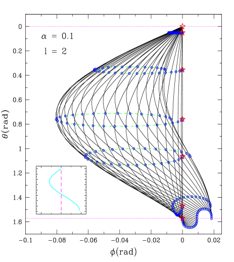
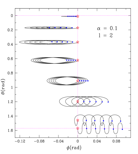
FIG. 1.:  Projected trajectories $\theta(t)\sin\theta(t)\cos\phi(t)$, and $\phi(t)\sin\theta(t)\cos\phi(t)$ of seven fiducial fluid elements as seen in the corotating frame. The left diagram shows the projected trajectories over one period of fiducial fluid elements subject to an $r$-mode oscillation with $\ell=2$, $\alpha=0.1$, and $\Omega=\Omega_{{}_{B}}$. All of the fluid elements are initially positioned on the $\phi_{0}=0$ meridian and have different latitudes (indicated with stars). Continuous lines show the simultaneous positions of the fluid elements and different lines refer to different times. The trajectories of some representative fluid elements are shown with dashed circles. The small inset in the left diagram of Fig. 1 shows the initial positions (dashed line) and final positions (continuous line) of the different fluid elements. The right panel uses the same quantities as in the left one, but shows the trajectories of eight fluid elements for five oscillations.

In Fig. 1 we show numerical integrations of the equations of motion (6) and (8) on the northern hemisphere of the rotating star. In particular, the left panel of Fig. 1 shows the projected $(\theta,\phi)$ trajectories over one period for fiducial fluid elements subject to an $r$-mode oscillation with $\ell=2$ (the coordinates are those of a reference frame corotating with the star). All of the fluid elements are initially positioned on the $\phi_{0}=0$ meridian, but at different latitudes and these positions are indicated with stars (because of the polar dependence of equations [6] and [8], it is sufficient to study them in the northern hemisphere only). The continuous lines show the simultaneous positions of fluid elements at different times (some of these positions are indicated with circles), and the dashed lines are used to trace the trajectories of representative fluid elements. In solving equations (6) and (8) we have assumed that $\alpha$ has the constant value $0.1$ and that the star is rotating at the break-up limit $\Omega_{{}_{B}}\equiv(2/3)\sqrt{\pi G{\bar{\rho}}}$, with ${\bar{\rho}}=3M/(4\pi R^{3})$ being the average mass density.

Several interesting properties can be deduced from Fig. 1: a) the trajectories over one period $\omega/2\pi$ are not closed; b) while the excursions in the $\theta$ and $\phi$ directions are comparable, the net displacement $\Delta\phi$ in longitude after one cycle is much larger than the net displacement $\Delta\theta$ in latitude (indeed one can show that this is zero at ${\cal O}(\alpha^{2})$); c) both $\Delta\phi$ and $\Delta\theta$ are linearly proportional to $\alpha$; d) the motions have a simple dependence on latitude. The small inset in the left diagram of Fig. 1 shows schematically the position of the fluid elements at the beginning of the oscillation (dashed line) and after one cycle (continuous line). The right panel of Fig. 1 shows the trajectories of fiducial fluid elements during five full oscillations and the net displacement produced by their motions.

Despite the complexity of the different trajectories, all of the information about their secular behaviour is contained in (11) and (12). These expressions are at the basis of our study of the interaction between $r$-mode oscillations and any magnetic field that is initially present in the rotating neutron star.

IV Evolution Equations for the Magnetic Field

In this Section we first discuss the model assumed for a magnetic neutron star (Section IV A) and then illustrate the techniques employed to compute the evolution of an arbitrarily small seed magnetic field as a result of the secular drift produced by the $r$-mode oscillations. In particular, we have considered both Lagrangian and Eulerian formulations of the induction equation. The first exploits the possibility of calculating the strain tensor produced by the oscillation. The second approach, on the other hand, is more commonly used and treats the induction equation as a set of partial differential equations. For compactness, the numerical results obtained using both of these methods are presented in Paper II.

A Simplified model of magnetic neutron stars

The properties of the magnetic fields of neutron stars still contain a number of unresolved aspects, mostly connected with the properties of matter at very high densities [25]. For simplicity, we will assume that the stellar magnetic field ${\mathbf{B}}$ is initially dipolar and aligned with the star’s spin axis. Then

$${\mathbf{B}}_{0}={\mathbf{B}}^{\hat{p}}(t=0)=B_{{}_{\rm d}}\frac{R^{3}}{r^{3}}\left(2\cos\theta{\mathbf{e}}_{\hat{r}}+\sin\theta{\mathbf{e}}_{\hat{\theta}}\right)\ ,$$ (13)

where $B_{{}_{\rm d}}$ is the strength of the equatorial magnetic field at the stellar surface and which is observed to be in the range $10^{11}-10^{13}$ G. The use of a dipolar magnetic field allows us to consider the star as being initially in magnetohydrostatic equilibrium and therefore avoids the calculation of a stable initial configuration. Moreover, we will assume that the electrical currents are concentrated at the origin and to avoid singularities we restrict our considerations to a region of the star with radius $pR\leq r\leq R$, where $0<p<1$, and $R$ is the stellar radius. Because any misalignment between the magnetic field and the rotation axis will only introduce geometrical corrections ${\mathcal{O}}(1)$, we expect that all of the features of the generation and evolution discussed below will not change significantly when a more generic initial configuration is considered.

Except for the very first moments after the star’s birth, the electrons in the outer layers of a neutron star are strongly degenerate and form an almost ideal Fermi-gas. Atoms are partially or fully ionized and form either a strongly coupled Coulomb liquid or a Coulomb crystal [26]. The electrical and thermal transport properties of this dense matter are mainly determined by the transport properties of the electrons, which are the most important carriers of electrical charge and heat. At temperatures above the crystallization temperature of the ions, the electrical and thermal conductivities are governed by electron scattering off ions. Increasingly accurate calculations of the electrical and thermal conductivity of the matter in hot neutron star envelopes can be found in the literature [26, 27, 28] and an approximate expression for the electrical conductivity is given by [25]

$$\sigma_{{}_{E}}\approx 10^{26}\left(\frac{10^{8}\ \rm K}{T}\right)^{2}\left(\frac{\rho}{10^{14}\ {\rm g\ cm}^{-3}}\right)^{3/4}\ {\rm s}^{-1}\ ,$$ (14)

where $T$ and $\rho$ are the stellar temperature and mass density. Even for a magnetic field that varies on a length-scale as small as $\Delta R\simeq 0.1R$, the magnetic diffusion timescale is

$$\tau_{\rm diff}=\frac{4\pi(\Delta R)^{2}\sigma_{{}_{E}}}{c^{2}}\approx 3\times 10^{6}\left(\frac{\Delta R}{10^{5}\ {\rm cm}}\right)^{2}\left(\frac{10^{9}\ \rm K}{T}\right)^{2}\left(\frac{\rho}{10^{14}\ {\rm g\ cm}^{-3}}\right)^{3/4}\ {\rm yr}\ .$$ (15)

This is well over six orders of magnitude larger than the one year timescale usually discussed for the existence of of $r$ modes for a typical newly-born neutron star. As a result, we can neglect the effects of Ohmic dissipation, treating the fluid as perfectly conducting on the timescales of interest here.

B Lagrangian approach

In order to simplify our notation, hereafter we will drop the index “1” for the linear velocity so that $\delta{\mathbf{v}}\equiv\delta{\mathbf{v}_{1}}$. Combining then the equation of mass conservation

$$\frac{d\rho}{dt}=-\rho\left(\nabla\cdot{\mathbf{v}}\right)\ ,$$ (16)

where $d/dt\equiv(\partial/\partial t+{\mathbf{v}}\cdot\nabla)$, with the induction equation

$$\frac{\partial{\mathbf{B}}}{\partial t}=\nabla\times\left({\mathbf{v}}\times{\mathbf{B}}\right)\ ,$$ (17)

one obtains

$$\frac{D}{Dt}\left(\frac{{\mathbf{B}}}{\rho}\right)=\left(\frac{{\mathbf{B}}}{\rho}\cdot\nabla\right)\delta{\mathbf{v}}\ ,$$ (18)

where we have decomposed the velocity ${\mathbf{v}}$ into ${\mathbf{v}}={\mathbf{v}}_{0}+\delta{\mathbf{v}}$, with ${\mathbf{v}}_{0}\equiv\Omega\times{\mathbf{r}}$ being the uniform stellar rotation velocity and $\delta{\mathbf{v}}$ the $r$-mode velocity perturbation. Here, ${D}/{Dt}\equiv({\partial}/{\partial t}+{\mathbf{v}}\cdot\nabla-{\mathbf{\Omega}}\times)$ is the Lagrangian derivative for a fluid element moving at velocity ${\mathbf{v}}$ as seen in the corotating frame. Equation (18) can be integrated analytically to give [15, 29] (see Appendix B for a derivation)

$$\frac{B^{j}}{\rho}({\tilde{\mathbf{x}}},t)=\frac{B^{k}}{\rho}({\mathbf{x}},t_{0})\frac{\partial{\tilde{x}}^{j}(t)}{\partial x^{k}(t_{0})}\ .$$ (19)

Note that $\nabla\cdot{\mathbf{v}}_{0}=0$ at first order in the stellar angular velocity and $\nabla\cdot\delta{\mathbf{v}}=0$ by definition of axial perturbations [cf. equations (* ‣ III A)]. To lowest order in $\Omega$ and $\alpha$ the flow is therefore incompressible and we can set $\rho({\tilde{\mathbf{x}}},t)=\rho({\mathbf{x}},t_{0})$. The integral form (19) of the induction equation is particularly advantageous as it shows that the magnetic field at time $t$ and position ${\tilde{\mathbf{x}}}$ can be computed from the magnetic field at time $t_{0}$ and position ${\mathbf{x}}$, using the tensorial coordinate strain $\partial{\tilde{x}}^{j}(t)/\partial{x}^{k}(t_{0})$ that develops between $t_{0}$ and $t$. The advection of magnetic field lines is an obvious consequence of Eq. (19) and the problem of the magnetic field evolution is therefore transformed into the problem of determining the time evolution of the strain tensor $S_{jk}\equiv\partial{\tilde{x}}^{j}/\partial{x}^{k}$. While very compact and relatively simpler to solve numerically, Eq. (19) has the disadvantage of being sensitive to the accurate calculation of the strain tensor, which might become difficult when the instability is fully developed. For this reason, and to verify the validity of the Lagrangian approach for very large saturation amplitudes, we have also implemented a more traditional Eulerian method for the solution of the induction equation which is discussed in the following Section.

C Orbit Average Eulerian approach

We start by rewriting the induction equation (17) as

$$\frac{{\mathcal{D}}{\mathbf{B}}}{{\mathcal{D}}t}=\nabla\times\left(\delta{\mathbf{v}}\times{\mathbf{B}}\right)=-\left(\delta{\mathbf{v}}\cdot\nabla\right){\mathbf{B}}+\left({\mathbf{B}}\cdot\nabla\right)\delta{\mathbf{v}}\ ,$$ (20)

where now ${\mathcal{D}}{\mathbf{B}}/{{\mathcal{D}}t}\equiv({\partial}/{\partial t}+{\mathbf{v}}_{0}\cdot\nabla-{\mathbf{\Omega}}\times){\mathbf{B}}=({D}/{Dt}-\delta{\mathbf{v}}\cdot\nabla){\mathbf{B}}$ is the time derivative of the magnetic field in a coordinate system instantaneously corotating with the star. Writing the directional derivatives in (20) explicitly within an orthonormal coordinate system $({\mathbf{e}}_{\hat{r}},{\mathbf{e}}_{\hat{\theta}},{\mathbf{e}}_{\hat{\phi}})$ gives

$$\frac{{\mathcal{D}}B^{\hat{r}}}{{\mathcal{D}}t}=-\delta v^{\hat{r}}\frac{\partial B^{\hat{r}}}{\partial r}+B^{\hat{r}}\frac{\partial\delta v^{\hat{r}}}{\partial r}+\frac{B^{\hat{\theta}}}{r}\frac{\partial\delta v^{\hat{r}}}{\partial\theta}-\frac{\delta v^{\hat{\theta}}}{r}\frac{\partial B^{\hat{r}}}{\partial\theta}+\frac{1}{r\sin\theta}\left(B^{\hat{\phi}}\frac{\partial\delta v^{\hat{r}}}{\partial\phi}-\delta v^{\hat{\phi}}\frac{\partial B^{\hat{r}}}{\partial\phi}\right)\ ,$$ (22)

(23)

$$\frac{{\mathcal{D}}B^{\hat{\theta}}}{{\mathcal{D}}t}=-r\delta v^{\hat{r}}\frac{\partial}{\partial r}\left(\frac{B^{\hat{\theta}}}{r}\right)+\,r\,B^{\hat{r}}\frac{\partial}{\partial r}\left(\frac{\delta v^{\hat{\theta}}}{r}\right)-\frac{\delta v^{\hat{\theta}}\sin\theta}{r}\frac{\partial}{\partial\theta}\left(\frac{B^{\hat{\theta}}}{\sin\theta}\right)+\frac{B^{\hat{\theta}}\sin\theta}{r}\frac{\partial}{\partial\theta}\left(\frac{\delta v^{\hat{\theta}}}{\sin\theta}\right)$$ (24)

$$\hskip 39.83368pt+\frac{1}{r\sin\theta}\left(B^{\hat{\phi}}\frac{\partial\delta v^{\hat{\theta}}}{\partial\phi}-\delta v^{\hat{\phi}}\frac{\partial B^{\hat{\theta}}}{\partial\phi}\right)\ ,$$ (25)

(26)

$$\frac{{\mathcal{D}}B^{\hat{\phi}}}{{\mathcal{D}}t}=-r\delta v^{\hat{r}}\frac{\partial}{\partial r}\left(\frac{B^{\hat{\phi}}}{r}\right)+\,r\,B^{\hat{r}}\frac{\partial}{\partial r}\left(\frac{\delta v^{\hat{\phi}}}{r}\right)-\frac{\delta v^{\hat{\theta}}\sin\theta}{r}\frac{\partial}{\partial\theta}\left(\frac{B^{\hat{\phi}}}{\sin\theta}\right)+\frac{B^{\hat{\theta}}\sin\theta}{r}\frac{\partial}{\partial\theta}\left(\frac{\delta v^{\hat{\phi}}}{\sin\theta}\right)$$ (27)

$$\hskip 39.83368pt+\frac{1}{r\sin\theta}\left(B^{\hat{\phi}}\frac{\partial\delta v^{\hat{\phi}}}{\partial\phi}-\delta v^{\hat{\phi}}\frac{\partial B^{\hat{\phi}}}{\partial\phi}\right)\ .$$ (28)

The induction equations (20) are not yet in a useful form since they refer to instantaneous values of the velocity perturbations. The magnetic field produced over a single oscillation is simply estimated to be $\delta B\approx\pi\alpha B$ and is uninterestingly small unless the seed magnetic field is already very large. We need therefore to perform an orbit average of the induction equations (20) over a timescale $\omega^{-1}\ll\tau\ll T$, where $T$ is the timescale for a global change of the velocity and magnetic fields. In this case we can introduce a time-average (secular) drift velocity ${\tilde{\mathbf{v}}}\equiv\langle\delta{\mathbf{v}}\rangle$, whose components at a time $t$ are defined as

$${\tilde{v}}^{\hat{i}}(r,\theta,\phi,t)\equiv\frac{1}{2\tau}\int^{\tau}_{-\tau}\delta v^{\hat{i}}(r,\theta,\phi,t+t^{\prime})\,dt^{\prime}\ ,\hskip 56.9055pti=2,\ 3.$$ (29)

and where, of course, ${\tilde{v}}^{\hat{r}}=0$. For simplicity and because of the smallness of $\delta{\mathbf{B}}$, we can neglect the nonlinear term $\nabla\times(\langle\delta{\mathbf{v}}\times\delta{\mathbf{B}}\rangle)$ introduced by the time average and correlating the velocity perturbation with the magnetic field perturbation. The orbit average of equations (20) then has the only effect of replacing $\delta v^{\hat{i}}$ with ${\tilde{v}}^{\hat{i}}$.

At this point a number of considerations can be made to simplify the solution of the orbit average of the Eulerian equations (20). Firstly, we note that the secular velocities must have the same variable separability as the originating instantaneous velocity perturbations. As a result, they can be similarly decomposed as [cf. Eq. (1)]

$${\tilde{v}^{i}}=f(r)g_{i}(\theta,\phi)=r^{\ell}g_{i}(\theta,\phi)\ ,\hskip 56.9055pti=2,~{}3\ ,$$ (30)

so that $\partial{\tilde{v}}^{\hat{i}}/\partial r=\ell{\tilde{v}}^{\hat{i}}/r$, and $\partial({\tilde{v}}^{\hat{i}}/r)/\partial r=(\ell-1){\tilde{v}}^{\hat{i}}/r^{2}$. By exploiting the property (30) we are therefore able to remove all of the radial derivatives in equations (20).

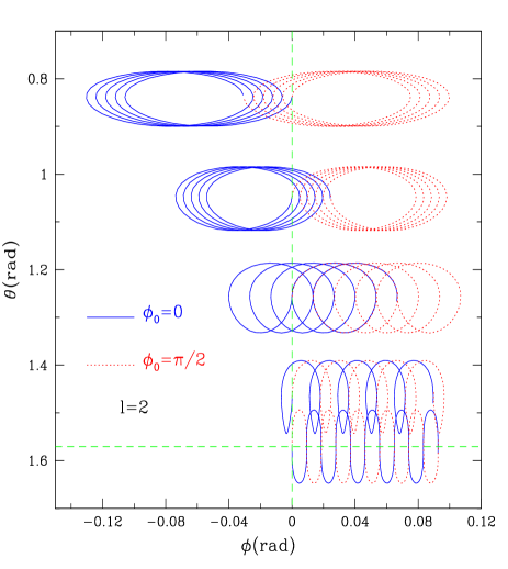
FIG. 2.:  This panel shows the trajectories $\theta(t)$, and $\phi(t)$ of fiducial fluid elements during five oscillations for a mode with $\ell=2$, $\alpha=0.1$, and $\Omega=\Omega_{{}_{B}}$. Continuous lines refer to fluid elements initially positioned on the $\phi_{0}=0$ meridian, while the dotted ones refer to fluid elements initially positioned on the $\phi_{0}=\pi/2$ meridian and have been rescaled as $\phi(t)\rightarrow\phi(t)-\pi/2$ in order to be superimposed on the same plot.

Secondly, while ${\tilde{v}}^{\hat{\phi}}$ has a polar dependence, it must be axisymmetric if it is continuous and periodic. This can most easily be seen by considering the equations of motion (* ‣ III A). In the case $\ell=2$, for instance, $\dot{\phi}$ will be periodic with period $\pi$ and will change sign at $\phi_{0}=\pi/2$. A similar $\pi$-periodicity must be expected also for ${\tilde{v}}^{\hat{\phi}}$ which, however, cannot change sign at $\phi_{0}=\pi/2$, nor vary as a function $\phi$, since either of these two features would make fluid elements converge secularly and thus produce discontinuities. This property of ${\tilde{v}}^{\hat{\phi}}$ is synthesized in Fig. 2, which shows the trajectories of fiducial fluid elements during five oscillations and the overall displacement that results from these motions (this is the same as the left panel of Fig. 1, but here we have considered only fluid motions near to the star’s equator). In particular, we show fluid trajectories for two different initial longitudes, i.e. $\phi_{0}=0$ and $\phi_{0}=\pi/2$, and rescale the latter trajectories so that they can be superimposed on the same plot. As expected, $\dot{\phi}$ has different signs for the two initial data, but in both cases ${\tilde{v}}^{\hat{\phi}}$ has the same sign, magnitude and polar dependence, so that we can set

$$\frac{\partial{\tilde{v}}^{\hat{\phi}}}{\partial\phi}=0\ .$$ (31)

Thirdly, while ${\tilde{v}}^{\hat{\theta}}$ does not have symmetries, it has some important properties: i) it has an overall periodic (in time) behaviour, with period $\gg 2\pi/\omega$; ii) the azimuthal dependence is of the form $e^{im\phi}$; iii) it is always much smaller than ${\tilde{v}}^{\hat{\phi}}$; iv) the polar dependence involves only the lowest order Legendre polynomials.

FIG. 3.:  Time evolution of the polar profile of ${\tilde{v}}^{\hat{\theta}}$ and ${\tilde{v}}^{\hat{\phi}}$ at the surface of the star and for an $\ell=2$ mode, saturated at an amplitude $\alpha_{\rm sat}=10^{-2}$. Different curves refer to different times and show the velocity increase produced by the growth of the mode amplitude. The velocity profiles shown here refer to a time $t<340$ s. The velocity and subsequently decreases as a result of the star’s spin down (not shown here).

This periodic behaviour of ${\tilde{v}}^{\hat{\theta}}$ guarantees that the polar deformations of the magnetic field are confined to very small scales and, when averaged over the relevant timescales, will produce negligible net effects.

Properties iii) and iv) are shown in Fig. 3 where we have plotted the evolution of the polar profiles for ${\tilde{v}}^{\hat{\theta}}$ and ${\tilde{v}}^{\hat{\phi}}$ at the surface of the star during the growth of an $\ell=2$ mode. Different curves refer to different times and show the progressive increase of ${\tilde{v}}^{\hat{\theta}}$ and ${\tilde{v}}^{\hat{\phi}}$ as a result of the mode’s growth. The largest velocity values are reached at saturation (which was here set to be $\alpha_{\rm sat}=10^{-2}$ and occurs at $t\simeq 340$ s) and it should be noted that ${\tilde{v}}^{\hat{\phi}}$ is almost two orders of magnitude larger than ${\tilde{v}}^{\hat{\theta}}$. Since both ${\tilde{v}}^{\hat{\theta}}$ and ${\tilde{v}}^{\hat{\phi}}$ depend linearly on $\Omega$ [cf. equations [* ‣ III A)], their values progressively decrease after saturation as a result of the star’s spin-down (This is not shown in Fig. 3.).

The azimuthal dependence of ${\tilde{v}}^{\hat{\theta}}$ is the same that would be imprinted on the magnetic field produced by the poloidal velocities. In fact, even an initially axisymmetric magnetic field would acquire non-axisymmetric features driven by ${\tilde{v}}^{\hat{\theta}}$. However, because these departures away from axisymmetry are always linearly dependent on ${\tilde{v}}^{\hat{\theta}}$ and on its $\phi$-derivative, we will assume them to be negligible and set

$$\frac{\partial{\tilde{v}}^{\hat{\theta}}}{\partial\phi}=\frac{\partial B^{\hat{r}}}{\partial\phi}=\frac{\partial B^{\hat{\theta}}}{\partial\phi}=\frac{\partial B^{\hat{\phi}}}{\partial\phi}=0\ .$$ (32)

As a result of (31), (32) and after some regrouping, the induction equations (20) take the form

$$\frac{{\mathcal{D}}B^{\hat{r}}}{{\mathcal{D}}t}=-\frac{{\tilde{v}}^{\hat{\theta}}}{r}\frac{\partial B^{\hat{r}}}{\partial\theta}\ ,$$ (34)

(35)

$$\frac{{\mathcal{D}}B^{\hat{\theta}}}{{\mathcal{D}}t}=\frac{B^{\hat{r}}{\tilde{v}}^{\hat{\theta}}}{r}-\frac{{\tilde{v}}^{\hat{\theta}}}{r}\frac{\partial B^{\hat{\theta}}}{\partial\theta}+\frac{B^{\hat{\theta}}}{r}\frac{\partial{\tilde{v}}^{\hat{\theta}}}{\partial\theta}\ ,$$ (36)

(37)

$$\frac{{\mathcal{D}}B^{\hat{\phi}}}{{\mathcal{D}}t}=\frac{B^{\hat{r}}{\tilde{v}}^{\hat{\phi}}}{r}-\frac{{\tilde{v}}^{\hat{\theta}}}{r}\frac{\partial B^{\hat{\phi}}}{\partial\theta}+\frac{{B}^{\hat{\theta}}}{r}\frac{\partial{\tilde{v}}^{\hat{\phi}}}{\partial\theta}+\left({\tilde{v}}^{\hat{\theta}}B^{\hat{\phi}}-B^{\hat{\theta}}{\tilde{v}}^{\hat{\phi}}\right)\frac{\cot\theta}{r}\ ,$$ (38)

The set of equations (32) has now only time and polar derivatives, and can be more easily solved numerically. Results of the numerical integration of (32) and of the comparison with results obtained from the Lagrangian approach will be presented in paper II. It is important to underline that the only approximation made in obtaining equations (32) from the more general equations (20) comes from ignoring the deviations away from axisymmetry in the velocity field. In this respect, dynamo theory and in particular Braginsky’s dynamo model [30], suggests that such an assumption can only lead to an underestimation of the actual growth rate of the magnetic field [31, 15].

The Eulerian or orbit average approach presented above is clearly more complicated to implement numerically than the corresponding Lagrangian method as it involves the use of a numerical grid on which the set of coupled partial differential equations needs to be solved. However, the Eulerian method has also been shown to be more accurate when the $r$-mode instability has reached saturation and the velocity perturbations at the star’s surface are ${\cal O}(\Omega R)$. In paper II we will present a close comparison of the two approaches discussed above.

D Simplified analytical model of the r-mode instability

While a detailed discussion of the full numerical calculations will be presented in paper II, in what follows we show how, with simple back of the envelope calculations, it is possible to predict the generation of very large toroidal magnetic fields as a result of the azimuthal secular velocity field produced by the onset and saturation of the $r$-mode instability. The estimates discussed below will then be confirmed by the full numerical calculations.

We start by considering the phenomenological expressions for the time evolution of the stellar angular velocity and the mode amplitude during the period of activity of the instability [12]. These can be summarized analytically as (see also Fig. 1 of paper II)

$$\Omega(t) = \left\{\begin{array}[]{ll}\Omega_{0}&\hskip 31.2982pt\textrm{~{}if \ $t\leq t_{\rm sat}$}\ ,\\ \Omega_{0}\left[1+C_{1}\Omega^{2\ell+2}_{0}(t-t_{\rm sat})\right]^{-(2\ell+2)}&\hskip 31.2982pt\textrm{~{}if \ $t>t_{\rm sat}$}\ ,\end{array}\right.$$ (41)

$$\alpha(t) = \left\{\begin{array}[]{ll}\alpha_{0}\;\textrm{exp}(t/|\tau_{{}_{\rm GW}}|)&\hskip 113.81102pt\textrm{if \ $t\leq t_{\rm sat}$}\ ,\\ \alpha_{\rm sat}&\hskip 113.81102pt\textrm{if \ $t>t_{\rm sat}$}\ .\end{array}\right.$$ (45)

Here $|\tau_{{}_{\rm GW}}|$ is the timescale for the onset of the instability, while $\Omega_{0}$ is the star’s initial angular velocity. $C_{1}$ is a short-hand for

$$C_{1}\equiv\frac{64\pi G}{c^{2\ell+3}}\frac{(2\ell+2)(\ell-1)^{2\ell}}{[(2\ell+1)!!]^{2}}\left(\frac{\ell+2}{\ell+1}\right)^{2\ell+2}\frac{Q\alpha^{2}_{\rm sat}}{1-Q\alpha^{2}_{\rm sat}}\int_{0}^{R}\rho\,r^{2\ell+2}dr\ ,$$ (47)

with $Q$ being a nondimensional quantity accounting for the internal structure of the star. For an $\ell=m=2$ mode [12]

$$Q\equiv\frac{9}{16\pi R^{2}}\left({\int^{R}_{0}\rho\,r^{6}dr}\right)\left({\int^{R}_{0}\rho\,r^{4}dr}\right)^{-1}\ .$$ (48)

Using (41) and (45), Eq. (11) can be integrated to give

$${\tilde{x}}^{\phi}(t)=\left\{\begin{array}[]{ll}\displaystyle\left(\frac{r}{R}\right)\frac{\kappa_{2}\Omega_{0}\alpha^{2}_{0}}{2}\,|\tau_{{}_{\rm GW}}|\biggl{[}\textrm{exp}(2t/|\tau_{{}_{\rm GW}}|)-1\biggr{]}\ ,&\hskip 21.33955pt\textrm{if \ $t\leq t_{\rm sat}$}\ ,\\ \\ \displaystyle\left(\frac{r}{R}\right)\frac{\kappa_{2}\Omega_{0}\alpha^{2}_{0}}{2}\,|\tau_{{}_{\rm GW}}|\biggl{[}\textrm{exp}(2t/|\tau_{{}_{\rm GW}}|)-1\biggr{]}\ +\\ \displaystyle\hskip 56.9055pt\left(\frac{6r}{5R}\right)\frac{(\kappa_{2})^{2}\alpha^{2}_{\rm sat}}{C_{1}\Omega^{5}_{0}}\biggl{\{}\left[1+C_{1}\Omega^{6}_{0}(t-t_{\rm sat})\right]^{5/6}-1\biggr{\}}\ ,&\hskip 21.33955pt\textrm{if \ $t>t_{\rm sat}$}\ .\end{array}\right.$$ (53)

Using Eq. (19), we can now estimate the average magnetic field produced at a given time at the surface of the star as a result of the secular drift (53). Assuming the initial magnetic field to be predominantly poloidal, i.e. $B^{\phi}({\mathbf{x}},t_{0})\ll B^{\theta}({\mathbf{x}},t_{0})$, the toroidal magnetic field produced is then

$$B^{\phi}({\tilde{\mathbf{x}}},t)=B^{r}({\mathbf{x}},t_{0})\frac{{\tilde{x}}^{\phi}(t)}{r}+B^{\theta}({\mathbf{x}},t_{0})\frac{\partial{\tilde{x}}^{\phi}(t)}{\partial\theta}\ .$$ (55)

For a “fiducial” neutron star, with mass $M=1.4{\rm M}_{\odot}$, radius $R=12.5$ km, and initial angular velocity $\Omega_{0}$ equal to $\Omega_{{}_{B}}$, the timescale for the onset of an unstable $\ell=m=2$ mode is then $|\tau_{{}_{\rm GW}}|\simeq 37$ s. If the initial perturbation has amplitude $\alpha_{0}=10^{-6}$, the mode will saturate at $\alpha_{\rm sat}=0.1$ after a time $t_{\rm sat}\simeq 430$ s [cf. Eq. (45)] and the volume averaged toroidal magnetic fields at saturation and after one year can be estimated to be respectively

$$\langle{\Delta B}^{\hat{\phi}}(t=t_{\rm sat})\rangle\simeq\int_{\rm V_{*}}\left[{B}^{\hat{r}}_{0}+\frac{2}{\pi}{B}^{\hat{\theta}}_{0}\right]{\tilde{x}^{\hat{\phi}}}{\;d^{3}{\bf x}}\sim 3.9\times 10^{2}\ \langle{B}^{\hat{p}}_{0}\rangle\ {\rm G}\ ,$$ (56)

(57)

$$\langle{\Delta B}^{\hat{\phi}}(t=1{\rm yr})\rangle\sim 1.2\times 10^{8}\ \langle{B}^{\hat{p}}_{0}\rangle\ {\rm G}\ ,$$ (58)

where $\langle({B}^{\hat{p}}_{0})^{2}\rangle\equiv\langle({B}^{\hat{r}}_{0})^{2}+({B}^{\hat{\theta}}_{0})^{2}\rangle$ is the initial poloidal magnetic field averaged over the stellar volume ${\rm V_{*}}$. Expressions (56) show that, in the absence of a back-reaction on the kinematics of the $r$-mode instability, the toroidal magnetic field is tightly wrapped around the star so as to have become about two orders of magnitude larger that the seed poloidal magnetic field in the short time necessary for the instability to reach saturation. Moreover, the total magnetic field could be amplified by eight orders of magnitude on a timescale of one year.

More detailed computations of the evolution of the magnetic field will be presented in paper II. However, the simple estimates outlined above already show that an initial magnetic field ${B}^{\hat{p}}_{0}$ could produce, after one year, an equipartition toroidal magnetic field of $\sim 10^{15}$ G, i.e. a toroidal magnetic field whose energy is comparable with the rotational energy of the star. Thus, an initial magnetic field exceeding $10^{8}$ G, (much below the measured magnetic field in young pulsars) would cause significant departures from the standard evolution of the $r$-mode instability. The impact of these very intense magnetic fields on the existence or growth of the $r$-mode oscillations will be discussed in detail in paper II. There, it will be possible to calculate the strength of the magnetic field necessary to significantly distort the first $r$-mode oscillation, or suppress the instability when this is free to develop.

V Conclusions

We have investigated the onset and growth of the $r$-mode instability in rotating magnetized neutron stars. Because of the high conductivity of the hot neutron star matter and the peculiar nature of the instability which is powered by large scale mass currents, it is not possible to ignore the presence of the strong magnetic fields that are expected to accompany newly born neutron stars.

Expanding the perturbed velocity field in powers of the mode amplitude we have derived a second-order analytic expression for a secular velocity field which we expect to emerge during the nonlinear growth of the instability. These secular motions produce a differential rotation both in the radial and in the polar directions. On an isobaric surface, the secular effects manifest themselves as a toroidal drift and couple with any pre-existing magnetic field to produce toroidal magnetic fields that rapidly grow in magnitude. In order to study how these kinematic effects interact with a magnetic field, we have discussed two different approaches to the solution of the induction equation and have derived sets of equations for the two cases. While we have left the discussion of the numerical results obtained to the companion paper II, we have here provided first estimates of the magnitudes of the magnetic fields that would be produced as a result of the shearing of a pre-existing poloidal magnetic field into a toroidal one. In particular, we have shown that it could be relatively simple to obtain, on the timescale usually discussed for the existence of the $r$-mode instability, magnetic fields that would be in equipartition the rotational kinetic energy of the star. The magnetic fields that are produced in this way will influence the $r$-mode instability either by preventing its onset (when sufficiently strong) or by suppressing its saturated development. Precise estimates of the critical magnetic field for prevention and damping of the instability will be presented in paper II.

A Equations of Motion: nonlinear effects from linearized equations

In this Appendix we outline the perturbative analysis which allows the periodic and secular parts in the linearized equations (* ‣ III A) to be distinguished. Here we will assume $\ell=2$, but the formalism presented can easily be generalized to the case of an arbitrary $\ell$. We start by rewriting (* ‣ III A) as

$${\dot{\theta}}(t,\theta,\phi)=\alpha A\sin\theta\cos\left(2\phi+\omega t\right)\ ,$$ (A4)

$${\dot{\phi}}(t,\theta,\phi)=-\alpha A\cos\theta\sin\left(2\phi+\omega t\right)\ ,$$

where

$$A\equiv\omega\left(\frac{r}{R}\right)c_{2}=\omega\left(\frac{r}{R}\right)\frac{1}{8}\sqrt{\frac{5!}{\pi}}\ .$$ (A5)

Next, we expand the solution of (A) in a series of powers of the mode amplitude $\alpha$, i.e. we look for solutions of the form

$${\theta}(t)=\phi_{0}+\alpha\phi_{1}(t)+\alpha^{2}\phi_{2}(t)+{\mathcal{O}}(\alpha^{3})\ ,$$ (A7)

(A8)

$${\phi}(t)=\theta_{0}+\alpha\theta_{1}(t)+\alpha^{2}\theta_{2}(t)+{\mathcal{O}}(\alpha^{3})\ .$$ (A9)

Substituting (A) into (A) yields

$${\dot{\theta}}(t,\theta,\phi)=\alpha A\bigg{\{}\left[\sin\theta_{0}\cos(\theta_{1}+\theta_{2})+\sin(\theta_{1}+\theta_{2})\cos\theta_{0}\right]\times$$ (A11)

$$\hskip 142.26378pt\left[\cos(2\phi_{0}+\omega t)\cos(2\phi_{1}+2\phi_{2})-\sin(2\phi_{0}+\omega t)\sin(2\phi_{1}+2\phi_{2})\right]\bigg{\}}\ ,$$ (A12)

(A13)

$${\dot{\phi}}(t,\theta,\phi)=-\alpha A\bigg{\{}\left[\cos\theta_{0}\cos(\theta_{1}+\theta_{2})-\sin(\theta_{1}+\theta_{2})\sin\theta_{0}\right]\times$$ (A14)

$$\hskip 142.26378pt\left[\sin(2\phi_{0}+\omega t)\cos(2\phi_{1}+2\phi_{2})+\cos(2\phi_{0}+\omega t)\sin(2\phi_{1}+2\phi_{2})\right]\bigg{\}}\ .$$ (A15)

where we have used the abbreviated notation of $\theta_{i}$ for $\alpha^{i}\theta_{i}$ and $\phi_{i}$ for $\alpha^{i}\phi_{i}$. Making use of the relations

$$\cos(\theta_{1}+\theta_{2})=1-\frac{\theta_{1}}{2}+{\mathcal{O}}(\alpha^{3})\ ,$$ (A16)

(A17)

$$\sin(\theta_{1}+\theta_{2})=\theta_{1}+\theta_{2}+{\mathcal{O}}(\alpha^{3})\ ,$$ (A18)

(A19)

$$\cos(2\phi_{1}+2\phi_{2})=1-2\phi^{2}_{1}+{\mathcal{O}}(\alpha^{3})\ ,$$ (A20)

(A21)

$$\sin(2\phi_{1}+2\phi_{2})=2(\phi_{1}+\phi_{2})+{\mathcal{O}}(\alpha^{3})\ ,$$ (A22)

equations (A) take the form

$${\dot{\theta}}(t,\theta,\phi)={\dot{\theta}_{0}}+{\dot{\theta}_{1}}+{\dot{\theta}_{2}}+{\dot{\theta}_{3}}+{\mathcal{O}}(\alpha^{4})\ ,$$ (A24)

(A25)

$${\dot{\phi}}(t,\theta,\phi)={\dot{\phi}_{0}}+{\dot{\phi}_{1}}+{\dot{\phi}_{2}}+{\dot{\phi}_{3}}+{\mathcal{O}}(\alpha^{4})\ ,$$ (A26)

where

$$\hskip 28.45274pt{\dot{\theta}}_{0}(t)=0\ ,$$ (A32)

$$\hskip 28.45274pt{\dot{\theta}}_{1}(t)=\alpha A\sin\theta_{0}\cos(2\phi_{0}+\omega t)\ ,$$

$$\hskip 28.45274pt{\dot{\theta}}_{2}(t)=\alpha A\left[\theta_{1}\cos\theta_{0}\cos(2\phi_{0}+\omega t)-2\phi_{1}\sin\theta_{0}\sin(2\phi_{0}+\omega t)\right]\ ,$$

and

$$\hskip-85.35826pt{\dot{\phi}}_{0}(t)=0\ ,$$ (A36)

$$\hskip-85.35826pt{\dot{\phi}}_{1}(t)=-\alpha A\cos\theta_{0}\sin(2\phi_{0}+\omega t)\ ,$$

$$\hskip-85.35826pt{\dot{\phi}}_{2}(t)=\alpha A\left[\theta_{1}\sin\theta_{0}\sin(2\phi_{0}+\omega t)-2\phi_{1}\cos\theta_{0}\cos(2\phi_{0}+\omega t)\right]\ \ .$$ (A38)

Note that, in principle, both $\alpha$ and $\omega$ (and therefore $A$) have a dependence on time which at first order in $\alpha$ produces orbits with increasing radius of gyration. Considering both $\alpha$ and $\omega$ as constant, we can easily find the integrals of equations (A) through an iterative procedure. In particular, we substitute into the right-hand-side of the equations for ${\dot{\theta}_{i}}(t)$ and ${\dot{\phi}_{i}}(t)$, the integrals of the equations for ${\dot{\theta}_{i-1}}(t)$ and ${\dot{\phi}_{i-1}}(t)$. By doing so we then obtain the following equations of motions

$$\hskip-99.58464pt{\ \theta}_{0}={\rm const.}\ ,$$ (A40)

$$\hskip-99.58464pt{\ \theta}_{1}(t)=\frac{\alpha A}{\omega}\sin\theta_{0}\sin(2\phi_{0}+\omega t)\ ,$$ (A44)

$$\hskip-99.58464pt{\ \theta}_{2}(t)=-\frac{\alpha^{2}A^{2}}{2\omega^{2}}\sin\theta_{0}\cos\theta_{0}\sin^{2}(2\phi_{0}+\omega t)\ ,$$

and

$$\hskip-28.45274pt{\ \phi}_{0}={\rm const.}\ ,$$ (A46)

(A47)

$$\hskip-28.45274pt{\ \phi}_{1}(t)=\frac{\alpha A}{\omega}\cos\theta_{0}\cos(2\phi_{0}+\omega t)\ ,$$ (A48)

(A49)

$$\hskip-28.45274pt{\ \phi}_{2}(t)=-\frac{\alpha^{2}A^{2}}{2\omega^{2}}\left[(2\phi_{0}+\omega t)\left(2\cos^{2}\theta_{0}-\sin^{2}\theta_{0}\right)+\sin(2\phi_{0}+\omega t)\cos(2\phi_{0}+\omega t)\left(2\cos^{2}\theta_{0}+\sin^{2}\theta_{0}\right)\right]\ ,$$ (A50)

(A51)

$$\hskip-28.45274pt{\ \phi}_{3}(t)=\alpha A\Bigg{[}2\phi^{2}_{1}\cos\theta_{0}\sin(2\phi_{0}+\omega t)-2\phi_{2}\cos\theta_{0}\cos(2\phi_{0}+\omega t)+$$ (A52)

$$\hskip 113.81102pt2\theta_{1}\phi_{1}\sin\theta_{0}\cos(2\phi_{0}+\omega t)+\theta_{2}\sin\theta_{0}\sin(2\phi_{0}+\omega t)\Bigg{]}\ .$$ (A53)

A rapid look at equations (A) and (A) shows that while ${\theta}_{1}(t)$, ${\theta}_{2}(t)$, and ${\ \phi}_{1}(t)$ are periodic functions, ${\theta}_{3}(t)$ and ${\ \phi}_{2}(t)$ have terms that grow linearly in time and are responsible for an ${\mathcal{O}}(\alpha^{3})$ drift in latitude and an ${\mathcal{O}}(\alpha^{2})$ drift in longitude.

As discussed in the main text, using equations (* ‣ III A) to compute the displacement of an element of fluid by expanding ${\dot{\theta}}$ and ${\dot{\phi}}$ in powers of $\alpha$ is not equivalent to considering nonlinear effects in the fluid equations. The key issue is whether the fluid drift given by (* ‣ III A) is at least qualitatively correct. In principle it might not be, because the velocity field obtained by solving the nonlinear fluid equations that describe $r$ waves might have additional parts that contribute to the drift and largely or completely cancel the drift given by the linear velocity field. Nonlinear solutions for the $r$ waves are not yet available, so it is natural to ask how the motions of fluid elements that we have found for the $r$ waves compare with the motions of fluid elements in other, more familiar waves.

Sound waves cause fluid elements to drift as well as to oscillate, as discussed by Landau and Lifshitz [20], who show how to compute the mass current density produced by a sound wave in the Eulerian frame, using the solution of the linearized fluid equations. The drift is of second-order in the wave amplitude. Calculating the fluid drift produced by sound waves as we have computed the drift produced by $r$ waves, i.e., by using the velocity field (* ‣ III A) in the Lagrangian frame to compute the motions of individual fluid elements, gives the drift quoted by Landau and Lifshitz. Shallow water waves are another interesting example. Here we outline how the fluid equations can be solved exactly for such waves, using the method of characteristics, and describe the exact solution. Consider an infinite train of shallow water waves with wavelength $2\pi k^{-1}$ much larger than the depth $h_{o}$ of the unperturbed water. The evolution of surface waves is then determined by the momentum and mass conservation equations

$$\frac{\partial u}{\partial t}+u\frac{\partial u}{\partial x}=-g\frac{\partial h}{\partial x}\qquad{\rm and}\qquad\frac{\partial h}{\partial t}+\frac{\partial(hu)}{\partial x}=0\ ,$$ (A54)

where $u$ is the horizontal velocity and $g$ is the gravitational acceleration. Using $c\equiv\sqrt{gh}$ instead of $h$, implicit solutions of arbitrary amplitude can be expressed in terms of the Riemann invariants, $I_{\pm}$, of the rightward-moving ($+$) characteristics and the leftward-moving ($-$) characteristics: $(dx/dt)_{\pm}=u\pm c$. Setting up at $t=0$ a right-propagating sinusoidal wave of small amplitude $y=\alpha c_{o}\cos(kx)$, $u=2\alpha c_{o}\cos(kx)$, where $y\equiv c-c_{o}$ and $c_{o}\equiv\sqrt{gh_{o}}$ is the speed of small-amplitude waves, we obtain for the right-moving characteristics $x(x_{o},t)=x_{o}+c_{o}[1+3\alpha\cos(kx_{o})]t$. As the wave propagates, the leading slopes of the crests steepen and form singularities at the earliest crossing of the characteristics, which occurs at $t_{\rm s}=1/3\alpha c_{o}k$. At early times ($t\ll t_{\rm s}$), we can use the above characteristic trajectory to obtain the velocity field to ${\cal O}\left(\alpha^{2}\right)$ from the exact solution. The result is $u=2\alpha c_{o}\cos k(x-c_{o}t)+3\alpha^{2}tkc_{o}^{2}\sin 2k(x-c_{o}t)$. Averaged over the period $T=2\pi/kc_{o}$, the first term gives the drift velocity $v_{\rm d}=2\alpha^{2}c_{o}$; the second term describes oscillations at twice the wave frequency, with the linearly growing amplitude $(3/2)v_{\rm d}c_{o}kt$. Subtracting constant-amplitude oscillations, the trajectory of a fluid element that is initially at $x_{o}$ is then $\bar{x}=x_{o}+v_{\rm d}t+(3/4)v_{\rm d}t\cos 2k(x_{o}-c_{o}t)$. Calculating the fluid drift produced by this wave in the same way we have done for the $r$ waves, i.e., using the velocity field $\delta{\vec{v}}_{1}$ in the Lagrangian frame to compute the motions of individual fluid elements, gives the same drift velocity as the exact solution, to second order in $\alpha$.

This calculation shows that shallow water waves produce a fluid drift and that the drift obtained by using the linear velocity field to compute the motion of an element of fluid is correct to second order in $\alpha$. Stated differently, when the full fluid equations that describe shallow water waves are solved exactly, one finds that the lowest-order nonlinear corrections to the linear velocity field, which includes all effects of ${\cal O}(\alpha^{2})$, make no contribution to the drift; the drift is given exactly to ${\cal O}(\alpha^{2})$ by the linear velocity field.

This result is so important that it may be worth restating it in a different way. Suppose that we solve the fluid equations for sound waves and shallow water waves exactly to ${\cal O}(\alpha^{2})$ and write the solution for the Eulerian velocity field as ${\vec{u}}(x,t)=\alpha{\vec{u}}_{1}+\alpha^{2}{\vec{u}}_{2}$. When evaluated at a fixed location, neither ${\vec{u}}_{1}$ nor ${\vec{u}}_{2}$ give a secular drift, i.e., a displacement that is linearly proportional to $t$. ${\vec{u}}_{1}$ is a pure sinusoid and therefore does not give a secular drift. ${\vec{u}}_{2}$ is a sinusoid that grows in amplitude and therefore does not give a secular drift either, because if at any time we wait one period longer, the displacement from the starting point given by ${\vec{u}}_{2}$ is in the opposite direction and even larger; the displacement given by ${\vec{u}}_{2}$ is not proportional to $t$. If now we compute the trajectory of an element of fluid by solving $d{\vec{x}}/dt={\vec{u}}({\vec{x}},t)$, we find that the only term that is proportional to $\alpha^{2}t$ arises from the $\alpha{\vec{u}}_{1}$ term in the Eulerian velocity field and from the fact that the velocity field at the position of the fluid element varies as it moves. The new part of the Eulerian velocity field that arises from solving the fluid equations to second order in $\alpha$ does not contribute to the secular drift to ${\cal O}(\alpha^{2})$; the secular drift is already given exactly to this order by the velocity field obtained by solving the linearized fluid equations.

We expect the drift of fluid elements that we have computed from the $r$-wave velocity field (* ‣ III A) to be qualitatively correct and perhaps exact to ${\cal O}(\alpha^{2})$.

B Magnetic field evolution equations: the Lagrangian approach

We here briefly show the derivation of the integral form of the induction equation (19) discussed in Section IV B. Consider a Lagrangian coordinate system ${\mathbf{x}}$. The differential equation (18) can then be written in terms of a generic vector field ${\mathbf{A}}$ as

$$\frac{D}{Dt}({\mathbf{A}})=({\mathbf{A}}\cdot\nabla)\delta{\mathbf{v}}\ .$$ (B1)

Equation (B1) can be readily integrated for an infinitesimal time interval $\delta t$ from an initial time $t_{0}$, so that

$$A^{i}(t_{0}+\delta t)=A^{i}(t_{0})+\left[A^{j}(t_{0})\frac{\partial v^{i}}{\partial x^{j}}\right]\delta t=A^{j}(t_{0})\frac{\partial}{\partial x^{j}}\biggl{[}x^{i}(t_{0})+v^{i}(t_{0})\delta t\biggr{]}=A^{j}(t_{0})\frac{\partial}{\partial x^{j}}\bigl{[}{\tilde{x}}^{i}(t_{0}+\delta t)\bigr{]}\ ,$$ (B2)

thereby relating the value of ${\mathbf{A}}$ at the new time $t+\delta t$, to the value of ${\mathbf{A}}$ at $t_{0}$. The extension of (B2) to a finite time interval is straightforward and yields

$$A^{j}({\tilde{\mathbf{x}}},t)=A^{k}({\mathbf{x}},t_{0})\left[\delta^{j}_{\ k}+\frac{\partial\Delta{\tilde{x}}^{j}(t)}{\partial x^{k}(t_{0})}\right]=A^{k}({\mathbf{x}},t_{0})\frac{\partial{\tilde{x}}^{j}(t)}{\partial x^{k}(t_{0})}\ ,$$ (B3)

where $\Delta{\tilde{x}}^{j}(t)={\tilde{x}}^{j}(t)-{\tilde{x}}^{j}(t_{0})={\tilde{x}}^{j}(t)-{x}^{j}(t_{0})$.

REFERENCES

- [1] L. Rezzolla, F. K. Lamb, and S. L. Shapiro, 1999, Astrophys. J. 531, L141 (2000).
- [2] L. Rezzolla, F. K. Lamb, D. Marković, and S. L. Shapiro, Phys. Rev. D, (2001), Paper II.
- [3] J. Papaloizou, and J. E. Pringle, MNRAS 182, 423 (1978).
- [4] J. Provost, G. Berthomieu, and A. Rocca, Astron. and Astrophys. 94, 126 (1981).
- [5] H. Saio, Astrophys. J. 256, 717 (1982).
- [6] N. Andersson, Astrophys. J. 502, 708 (1998).
- [7] J. F. Friedman, and Morsink, S. M., Astrophys. J. 502, 714 (1998).
- [8] N. Andersson, and K. D. Kokkotas, Int. Journ. of Mod. Phys. D, in press (2000).
- [9] J. F. Friedman and K. H. Lockitch 2001, Proceedings of the IX Marcel Grossman Meeting, World Scientific, eds. V. Gurzadyan, R. Jantzen, R. Ruffini; gr-qc/0102114.
- [10] L. Lindblom, B. J. Owen, and S. M. Morsink, Phys. Rev. Lett. 80, 4843 (1998).
- [11] N. Andersson, K. D. Kokkotas, and B. F. Schutz, 1999, Astrophys. J. 510, 846
- [12] B. J. Owen, L. Lindblom, C. Cutler, B. F. Schutz, A. Vecchio, and N. Andersson, Phys. Rev. D 58, 084020 (1998).
- [13] W. C. G. Ho and D. Lai, Astrophys. J. 543, 386 (2000).
- [14] G. Mendell, Phys. Rev. D, in press, gr-qc/0102042 (2001).
- [15] E. N. Parker, Cosmical Magnetic Fields, Clarendon Press, Oxford, Great Britain (1979) § 4.3.
- [16] H. C. Spruit, Astron. and Astrophys. 341, L1 (1999).
- [17] K. Schenk et al. gr-qc/0101092 (2001).
- [18] K. S. Thorne, Rev. Mod. Phys. 52, 299 (1980).
- [19] L. Lindblom, G. Mendell, and B. J. Owen, Phys. Rev. D 60, 064006 (1999).
- [20] L. D. Landau, L. D., & E. M. Lifshitz, Fluid Mechanics, Pergamon Press, Oxford, Great Britain (1987), § 65.
- [21] J. Lighthill, Waves in Fluids, Cambridge Univ. Press, Cambridge, Great Britain (1980), p. 279.
- [22] Y. Levin and G. Ushomirsky, Mon. Not. R. Astr. Soc. 322, 515 (2001).
- [23] N. Stergioulas, J. A. Font, Phys. Rev. Lett. 86, 1148 (2001).
- [24] L. Lindblom, J. E. Tohline, and M. Vallisneri, Phys. Rev. Lett. 86, 1152 (2001).
- [25] F. K. Lamb, in Frontiers of Stellar Evolution, ed. D. L. Lambert, Astronomical Society of the Pacific, (1991).
- [26] D. G. Yakovlev, V. A. Urpin, SvA 24, 303 (1980).
- [27] N. Itoh, H. Hayashi, and Y. Kohyama, Astrophys. J. 418, 405 (1993).
- [28] A. Y. Potekhin, D. A. Baiko, P. Haensel, D. G. Yakovlev, Astron. and Astrophys. 346, 345 (1999).
- [29] S. A. Balbus, and J. F. Hawley, Rev. Mod. Physics 70, 1 (1998).
- [30] S. I. Braginsky, Sov. Phys. JETP 20, 726 (1964).
- [31] H. K. Moffatt, Magnetic Field Generation in Electrically Conducting Fluids, Cambridge Univ. Press, Cambridge, Great Britain, p. 179 (1978).