Bounce behaviour in Kantowski-Sachs and Bianchi Cosmologies

Abstract

Many cosmological scenarios envisage either a bounce of the universe at early times, or collapse of matter locally to form a black hole which re - expands into a new expanding universe region. Energy conditions preclude this happening for ordinary matter in general relativistic universes, but scalar or dilatonic fields can violate some of these conditions, and so could possibly provide bounce behaviour. In this paper we show that such bounces cannot occur in Kantowski - Sachs models without violating the reality condition $\dot{\phi}^{2}\geq 0$. This also holds true for other isotropic spatially homogenous Bianchi models, with the exception of closed Friedmann - Robertson - Walker and Bianchi IX models; bounce behaviour violates the weak energy condition $\rho\geq 0$ and $\rho+p\geq 0$. We turn to the Randall-Sundrum type braneworld scenario for a possible resolution of this problem.

1 Introduction

Already in the 1930’s, Tolman [1] proposed that closed ($k=+1$) Friedmann - Robertson - Walker (FRW) universe models might re - expand after collapsing towards a high density state in the future; it was already known then that this was not possible for $k=0$ and $k=-1$ models. This idea of a “phoenix universe” has remained popular (see Dicke and Peebles [2] for a discussion), and has re - appeared recently in new forms, for example specifically in Smolin’s idea of collapse to a black hole state resulting in re - expansion into a new expanding universe region [3] and more recently Easson and Brandenberger [4] have discussed the general features all such scenarios have in common. Thus it is interesting to investigate under what conditions such a bounce might take place within the context of General Relativity and other theories of gravity (see for example [5]).

Essentially because of the Raychaudhuri equation [6, 7, 8], such bounces are not possible in FRW models if the active gravitational mass is positive: that is, if $\rho+3p>0$. On the other hand quantum fields and indeed classical scalar fields can violate this condition [9]. Hence such fields can in principle allow bounce behaviour in FRW models. However there are still other conditions that must be satisfied by such fields, for example the reality condition (RC) $\dot{\phi}^{2}\geq 0$ which is equivalent to requiring that the inertial mass density $\rho+p\geq 0$ (if this is not true, very anomalous physical behaviour can occur). Thus it is interesting to see when bounces can occur without violating such conditions.

It is not only FRW models that are of interest. The geometry of the universe at a bounce might be very different than the completely isotropic and spatially homogeneous FRW spacetimes; indeed because some spatially homogeneous modes are unstable [10], some more general geometry might be expected. Thus it is interesting to examine also what happens in models such as Bianchi models which are anisotropic and spatially homogeneous, in order to start exploring the full phase - space of possibilities. Additionally, in the scenario of black hole collapse and subsequent re - expansion, we might expect the geometry at the bounce to be that of a Kantowski - Sachs $k=+1$ model [11, 12], because this model has the same symmetries as the spatially homogeneous interior region of the extended (vacuum) Kruskal solution that represents the late stage of evolution of an isotropic black hole when the matter can be neglected. We may indeed expect that at late stages of collapse such a vacuum approximation will be valid, because in many Bianchi universes anisotropy dynamically dominates over matter at early and late times [10].

For these reasons we are interested in the bounce behaviour not only of FRW models but also of Bianchi and Kantowski - Sachs universes. In this paper, we prove a number of relevant results. Specifically, bounce behaviour in LRS Bianchi types I (BI) and III (BIII) or Kantowski - Sachs (KS) models with scalar fields violate the reality condition $\dot{\phi}^{2}=\rho+p\geq 0$ (we assume that the energy flux and anisotropic pressure vanish: $\pi_{\mu\nu}=0=q_{\mu}$ which follows for fields observed relative to the normal congruence of curves). For scalar field models with arbitrary self - interaction we prove a no - bounce theorem to this effect, viz. bounce behaviour in LRS BI, BIII or KS models violates the reality condition .

We then present additional results that restrict bounce behaviour in other spatially homogeneous models to closed FRW and Bianchi type IX. Open FRW and all (un-tilted) spatially homogeneous models all violate the weak energy condition (WEC) $\rho\geq 0$ and $\rho+p\geq 0$ at the time of a bounce. The strong energy condition (SEC) is violated in all such models, including flat FRW models. The RC and the null energy condition are violated in all spatially homogeneous models with the exception of Bianchi type IX and closed FRW models.

Finally we turn our attention to the braneworld scenario of Randall and Sundrum [13]. For a Kantowski-Sachs, BI or BIII metric confined to a single three-brane embedded in a five-dimensional bulk, a non - local anisotropic pressure and negative non - local energy density (e.g. dark radiation) projected from the bulk onto the brane via the bulk Weyl tensor modifies the Einstein field equations sufficiently for bounce behaviour to be consistent with the RC.

We should also mention efforts to solve the standard cosmological puzzles such as the flatness, homogeneity and monopole problems via ekpyrotic models [14] in the braneworld context as potential alternatives to inflation despite being plagued with their own difficulties. In particular there has been considerable discussion in the literature on the evolution of cosmological perturbations through a bounce in the ekpyrotic scenario (see [15] for a representative sample). This issue although extremely interesting, does not directly related to main the aims of this paper.

2 The Key Equations

In this section we set up the equations needed to investigate whether or not the dynamics of LRS BI, BIII and KS models admit bounce behaviour in the presence of a classical minimally coupled scalar field $\phi$ with a self - interaction potential $V(\phi)$. The metric tensor for these models can be written in the following form:

$$ds^{2}=-dt^{2}+X(t)^{2}dr^{2}+Y(t)^{2}(d\theta^{2}+S^{2}(\theta)d\phi^{2})\;,$$ (1)

where

$$S(\theta)=\left\{\begin{array}[]{c}\sin{\theta}~{}~{}\textstyle{for}~{}~{}k=+1\;,\cr\theta~{}~{}\textstyle{for}~{}~{}k=0\;,\cr\sinh{\theta}~{}~{}\textstyle{for}~{}~{}k=-1\;,\end{array}\right.$$ (5)

$X(t)$ and $Y(t)$ are the expansion scale factors and we have chosen standard units where $8\pi G=c=1$.

Relative to a normal congruence of curves with tangent vector $u^{\mu}$, the energy - momentum tensor $T_{\mu\nu}$ for a scalar field takes the form of a perfect fluid (See [10] page 17 for details):

$$T_{\mu\nu}=\rho u_{\mu}u_{\nu}+ph_{\mu\nu}\,,$$ (6)

with

$$\rho=\textstyle\frac{1}{2}\dot{\phi}^{2}+V(\phi)$$ (7)

and

$$p=\textstyle\frac{1}{2}\dot{\phi}^{2}-V(\phi)\;.$$ (8)

It is easy to show that for the above metric and choice of $u^{\mu}$, the Einstein field equations can be written in terms of propagation equations for the usual expansion $\Theta$, shear $\sigma^{2}=\frac{1}{2}\sigma^{\mu\nu}\sigma_{\mu\nu}$ and 3 - curvature ${}^{(3)}R$ scalars:

$$\dot{\Theta}+\textstyle\frac{1}{3}\Theta^{2}+2\sigma^{2}+\dot{\phi}^{2}-V(\phi)=0\;,$$ (9)

$$\dot{\sigma}+\Theta\sigma-\textstyle\frac{1}{2\sqrt{3}}{}^{(3)}R=0\;,$$ (10)

$${}^{(3)}\dot{R}+\textstyle\frac{2}{3}\Theta{}^{(3)}R-\textstyle\frac{2}{\sqrt{3}}{}^{(3)}R\sigma=0\;,$$ (11)

and the Gauss - Codazzi constraint

$${}^{(3)}R=\dot{\phi}^{2}+2V(\phi)+2\sigma^{2}-\textstyle\frac{2}{3}\Theta^{2}\;,$$ (12)

where

$$\Theta=\frac{\dot{X}}{X}+\frac{2\dot{Y}}{Y}\;,~{}~{}~{}~{}\sigma=\frac{1}{\sqrt{3}}\left(\frac{\dot{X}}{X}-\frac{\dot{Y}}{Y}\right)\;,~{}~{}{}^{(3)}R=\frac{2k}{Y^{2}}\;,$$ (13)

and $k$ is a constant taking the values $k=0,-1,+1$ for BI, BIII and KS models respectively. The above set of equations together with the Klein - Gordon equation

$$\ddot{\phi}+\Theta\dot{\phi}+\frac{\partial V}{\partial\phi}=0$$ (14)

give a complete description of the dynamics of these universe models and solutions may be obtained once $V(\phi)$ has been specified. The expansion may also be expressed in terms of a volume scale factor $a(t)$, viz. $\Theta={3\dot{a}\over a}$.

It is worth mentioning that there is an alternate route to finding solutions by noticing that equations (9) and (12) can be combined to give expressions for the potential and momentum density of the scalar field:

$$V(\phi) = \textstyle\frac{1}{3}(\dot{\Theta}+\Theta^{2}+{}^{(3)}R)\;,$$ (15)

$$\dot{\phi}^{2} = -\textstyle\frac{2}{3}\dot{\Theta}-2\sigma^{2}+\textstyle\frac{1}{3}{}^{(3)}R\;,$$ (16)

so that in principle $V(\phi)$ can be determined by first specifying the scale factor dependence $X(t)$ and $Y(t)$ and then running the field equations backwards to determine the potential. This method has been used to generate exact FRW inflationary solutions [16].

The aim here is not to attempt to find exact solutions but examine whether it is possible to find solutions that exhibit bounce behaviour subject to the RC: $\dot{\phi}^{2}\geq 0$. Hence we need a precise definition of what a bounce is, together with a careful examination of equation (16). This is discussed in the next section.

3 The No - bounce theorem in BI, BIII and KS models

3.1 Definition of a Bounce

Defining the expansion parameters

$$x=\dot{X}/{X}\;,~{}~{}~{}y=\dot{Y}/{Y}\;,$$ (17)

a bounce in $X$ occurs at time $t=t_{0}$ iff $x(t_{0})=0$ and $\dot{x}(t_{0})>0$ while a bounce in $Y$ occurs at time $t=t_{1}$ iff $y(t_{1})=0$ and $\dot{y}(t_{1})>0$. It is clear that although it may be possible to have a bounce in one of the scale factors but not the other, this does not lead to a new expanding universe region. We therefore require that a bounce occurs both in $X$ and $Y$ scale - factors, even though they may in general occur at different times.

3.2 The reality condition at a bounce

Let us now determine whether the RC for the scalar field is satisfied at a bounce. In order to do this we need to write equation (16) in terms of $x$ and $y$ and their derivatives. This is most easily done by first substituting for the spatial curvature ${}^{(3)}R$ using equation (10):

$$\dot{\phi}^{2}=-\textstyle\frac{2}{3}\dot{\Theta}-2\sigma^{2}+\textstyle\frac{2}{\sqrt{3}}\dot{\sigma}+\textstyle\frac{2}{\sqrt{3}}\Theta\sigma\;.$$ (18)

Now using

$$\sigma=\textstyle\frac{1}{\sqrt{3}}(x-y)\;,~{}~{}~{}~{}\Theta=x+2y\;,$$ (19)

we obtain

$$\dot{\phi}^{2}=-2(\dot{y}+y^{2}-xy)\;.$$ (20)

We can now state and prove the main result of this section .

Theorem: Bounce behaviour in LRS Bianchi type I, III and Kantowski - Sachs models dominated by a minimally coupled scalar field is not permitted unless the RC $\dot{\phi}^{2}\geq 0$ is violated.

Proof: The proof follows immediately from equation (20) when evaluated for a bounce in the $Y$ direction at time $t=t_{1}$. In this case $y(t_{1})=0$ and $\dot{y}(t_{1})>0$ so (20) simplifies to give $\dot{\phi}(t_{1})^{2}=-2\dot{y}(t_{1})<0$, so that even if a bounce occurs in the $X$ direction it is only possible in the $Y$ direction if the RC is violated.

4 No bounce behaviour in other Bianchi models

We now examine the extent to which energy conditions preclude bounce behaviour in isotropic, spatially homogeneous Bianchi models of class A and B. We refer the reader to Wainwright and Ellis [10] for an interesting review and classification of Bianchi type universes. Wald’s no-hair theorem for global anisotropy can be found in [18].

Not all Bianchi type models isotropize at large times. Specifically, those types which do not admit FRW solutions become highly anisotropic [19]. Models that do admit FRW solutions; Bianchi I and $VII_{0}$ admits k=0 solutions, Bianchi V and $VII_{h}$ admits $k=-1$ solutions, and Bianchi IX admits $k=+1$ solutions. Type $VII_{h}$ will in general not approach isotropy, while the type IX models will recollapse after a finite time.

From the outset it is clear that bounce behaviour in the volume scale factor $a(t)$ violates the SEC. This can be seen from the Raychaudhuri equation for spatially homogeneous cosmologies

$$\dot{\Theta}+\textstyle{{1\over 3}}\Theta^{2}+2\sigma^{2}=-\textstyle{{1\over 2}}(\rho+3p)\;,$$ (21)

which simplifies to

$$-\textstyle{{1\over 2}}(\rho+3p)=\dot{\Theta}(t_{0})+2\sigma^{2}(t_{0})>0\;,$$ (22)

since $\Theta=0$ at the bounce in the volume scale factor, and positivity results from $\sigma^{2}$ being non-negative, together with the requirement that $\dot{\Theta}>0$ at the bounce. Hence $\rho+3p<0$, violating the SEC at the bounce.

In addition to this, bounce behaviour in spatially homogeneous models with negative spatial curvature ${}^{(3)}R$ violates the WEC $\rho\geq 0$ and $\rho+p\geq 0$. To show this we use the Friedmann constraint for spatially homogeneous cosmologies

$$\rho+\sigma^{2}=\textstyle{{1\over 3}}\Theta^{2}+\textstyle{{1\over 2}}{}^{(3)}R\;,$$ (23)

which simplifies to $\rho+\sigma^{2}=\textstyle{{1\over 2}}{}^{(3)}R<0$ at the bounce, implying that $\rho<0$, since $\sigma^{2}$ is non-negative. This violates the WEC in class A types II, $VI_{0}$, $VII_{0}$ (except for a very special case) and VIII. Bounce behaviour can be obtained in type IX models, which can have positive curvature. In class B, the spatial curvature is negative for all models, hence the WEC is violated in all class B models.

Finally, spatially homogeneous cosmologies satisfy the RC provided that

$$\dot{\phi}^{2}=\textstyle{{1\over 3}}{}^{(3)}R-\textstyle{{2\over 3}}\dot{\Theta}-2\sigma^{2}\geq 0\ .$$ (24)

This constraint (c.f equation 13) is obtained by subtracting equations (21) and (23), and then rearranging terms. Bounce behaviour implies that $\textstyle{{2\over 3}}\dot{\Theta}+2\sigma^{2}>0$, since the shear $\sigma^{2}$ is non-negative. Hence we can write condition (24) in a somewhat weaker from, viz. Models satisfying the RC necessarily have ${}^{(3)}R>0$. Therefore, spatially homogeneous cosmologies with ${}^{(3)}R\leq 0$ violate the RC. This does not mean models with positive spatial curvature necessarily satisfy the RC, since they have to meet the stronger condition (24), in cases where the shear is non-vanishing at the time of the bounce. However, for isotropic models, it is necessary and sufficient that the spatial curvature is positive.

Bianchi class A types II, $VI_{0}$ and VIII all have negative spatial curvature, and for type I it is zero. Type $VII_{0}$ is negative or zero. Hence all these cases violate the RC, by virtue of the above argument. Type IX violates the RC for cases in which the spatial curvature is negative or zero.

In class B, since types IV, V, $VI_{h}$ and $VII_{h}$ have negative spatial curvature. Bianchi III is the special case of $h=-1$ in Bianchi $VI_{h}$, and the exceptional case Bianchi $VI^{*}_{-1/9}$ has $h=-1/9$. They all violate the RC.

5 Bounce behaviour on a Kantowski-Sachs brane

Recent ideas in string and M -theory [20, 21, 22] have led to the notion that gravity could be a higher dimensional theory, that becomes 4-dimensional at low energies. In the Randall-Sundrum scenario [13] gravity can be localised on a 3-brane while a fifth dimension may remain non-compact. Observers are bound to a brane, which may have a more general metric than the induced Minkowski metric that Randall and Sundrum [13] assumed. A covariant geometric approach was first given by Shiromizu, Maeda and Sasaki [21] and also by Maartens [23]. We shall assume that a scalar field $\phi$ is bound to the brane, and that and higher-dimensional modifications of the standard Einstein field equations are imprinted via (i) local quadratic energy-momentum corrections that arise from the extrinsic curvature, and (ii) non - local effects from the free gravitational field in the bulk, transmitted via a projection of the bulk Weyl tensor onto the brane [23].

In five dimensions, the field equations [13, 23] are Einstein’s equations, with a (negative) bulk cosmological constant $\widetilde{\Lambda}$ and the brane energy - momentum providing the source:

$$\widetilde{G}_{AB}=\widetilde{\kappa}^{2}\left[-\widetilde{\Lambda}\widetilde{g}_{AB}+\delta(\chi)\left\{-\lambda g_{AB}+T_{AB}\right\}\right]\,.$$ (25)

The tildes denote the bulk (5 - dimensional) generalisation of standard general relativity quantities, and $\widetilde{\kappa}^{2}=8\pi/\widetilde{M}_{\rm p}^{3}$, where $\widetilde{M}_{\rm p}$ is the fundamental 5 - dimensional Planck mass, which is typically much less than the effective Planck mass on the brane, $M_{\rm p}=1.2\times 10^{19}$ GeV. The brane is given by $\chi=0$, so that a natural choice of coordinates is $x^{A}=(x^{\mu},\chi)$, where $x^{\mu}=(t,x^{i})$ are spacetime coordinates on the brane. The brane tension is $\lambda$, and $g_{AB}=\widetilde{g}_{AB}-n_{A}n_{B}$ is the induced metric on the brane, with $n_{A}$ the spacelike unit normal to the brane. Matter fields confined to the brane make up the brane energy - momentum tensor $T_{AB}$ (with $T_{AB}n^{B}=0$).

The modification to the standard Einstein equations [23], with the new terms carrying bulk effects onto the brane are

$$G_{\mu\nu}=-\Lambda g_{\mu\nu}+T_{\mu\nu}+\widetilde{\kappa}^{4}S_{\mu\nu}-{\cal E}_{\mu\nu}\,.$$ (26)

If $\lambda={6\over\widetilde{\kappa}^{4}}$, then the energy scales are related as follow:

$$\Lambda={1\over 2}\widetilde{\kappa}^{2}\left(\widetilde{\Lambda}+{1\over 6}\widetilde{\kappa}^{2}\lambda^{2}\right)\;.$$ (27)

The tensor $S_{\mu\nu}$ represents local quadratic energy - momentum corrections of the matter fields, and the ${\cal E}_{\mu\nu}$ is the projected bulk Weyl tensor transmitting non - local gravitational degrees of freedom from the bulk to the brane. All the bulk corrections may be consolidated into effective total energy density $\rho^{tot}$, pressure $p^{tot}$, anisotropic stress $\pi^{tot}_{\mu\nu}$ and energy flux $q^{tot}_{\mu}$. The modified Einstein equations take the standard Einstein form with a redefined energy - momentum tensor:

$$G_{\mu\nu}=-\Lambda g_{\mu\nu}+T^{\rm tot}_{\mu\nu}\,,$$ (28)

where

$$T^{\rm tot}_{\mu\nu}=T_{\mu\nu}+\widetilde{\kappa}^{4}S_{\mu\nu}-{\cal E}_{\mu\nu}\,.$$ (29)

5.1 Matter description on the Kantowski-Sachs brane

A homogeneous scalar field $\phi(t)$ on the brane has an energy - momentum tensor given by equations (6)-(8), and in the absence of local anisotropic pressure and energy flux $\pi_{\mu\nu}=0=q_{\mu}$, effective total energy - momentum tensor has

$$\rho^{\rm tot} = \rho+{\rho^{2}\over 2\lambda}+\rho_{*}\,,$$ (30)

$$p^{\rm tot} = p+\rho(p+{\rho\over 2\lambda})+\textstyle\frac{1}{3}\rho_{*}$$ (31)

with a non - local energy density $\rho_{*}=-{\cal E}_{\mu\nu}u^{\mu}u^{\nu}$. A thorough analysis of the dynamics of FRW, Bianchi I and V models obeying a barotropic equation of state on the brane was done by Campos and Sopuerta [24] and for a scalar field by Goheer and Dunsby [25]. A Kantowski-Sachs brane is characterised by vanishing acceleration, vorticity and non - local energy flux (similar to that for a Bianchi I brane, but with positive 3-curvature; see for instance [23, 26]):

$$A^{\mu}=\omega^{\mu}=q^{\mu}_{*}=0\;,$$ (32)

hence the total energy flux vanishes

$$q_{\rm tot}^{\mu}=0\,.$$ (33)

However, the anisotropic stress does not necessarily vanish:

$$\pi^{\rm tot}_{\mu\nu}=\pi^{*}_{\mu\nu}\,.$$

Here $\pi^{*}_{\mu\nu}=-(h_{\mu}^{\ \alpha}h_{\nu}^{\ \beta}-{1\over 3}h^{\ \alpha\beta}h_{\mu\nu}){\cal E}_{\alpha\beta}$. There is no evolution equation for $\pi^{*}_{\mu\nu}$ on the brane, since the non - local anisotropic stress carry bulk degrees of freedom that cannot be determined by brane observers. In general, the projection of the five-dimensional field equations onto the brane, together with the $Z_{2}$ symmetry, does not lead to a closed system. The standard conservation equation of general relativity holds on the brane, together with a simplified propagation equation for the non - local energy density $\rho_{*}$ [23, 26]:

$$\dot{\rho}+\Theta(\rho+p)=0\,,$$ (34)

$$\dot{\rho}_{*}+{\textstyle{4\over 3}}\Theta{\rho}_{*}+\sigma_{\mu\nu}\pi_{*}^{\mu\nu}=0\,,$$ (35)

where $\Theta$ is the expansion parameter. Both $\rho_{*}$ and $\pi^{*}_{\mu\nu}$ are homogeneous on the brane.

5.2 Gravitational Equations

The Einstein Field equations (9)-(12) of section 2 are modified:

$$\dot{\Theta}+{\textstyle{1\over 3}}\Theta^{2}+2\sigma^{2}+{\textstyle{1\over 2}}(\rho+3p)=\Lambda-{\textstyle{1\over 2}}(2\rho+3p)\textstyle\frac{\rho}{\lambda}-\rho_{*}\;,$$ (36)

$$\dot{\sigma}+\Theta\sigma-{\textstyle{1\over 2\sqrt{3}}}{}^{(3)}R=\textstyle\frac{1}{2}\textstyle\frac{\sigma_{\mu\nu}\pi_{*}^{\mu\nu}}{\sigma}\,,$$ (37)

$${}^{(3)}\dot{R}+{\textstyle{2\over 3}}\Theta{}^{(3)}R-{\textstyle{2\over\sqrt{3}}}{}^{(3)}R\sigma=0\,,$$ (38)

$${\textstyle{2\over 3}}\Theta^{2}+{}^{(3)}R-2\sigma^{2}=2\Lambda+2\rho\left(1+{\textstyle{\rho\over 2\lambda}}\right)+2\rho_{*}\,.$$ (39)

The effects of embedding the free gravitational field in the five - dimensional bulk are represented by the correction terms to the energy - momentum tensor $T_{\mu\nu}$, as expressed in equations (36), (37) and (39).

5.3 Feasible Bounce Behaviour

If we subtract equation (39) from $2$ $\times$ equation (36):

$$(1+\textstyle\frac{\rho}{\lambda})(\rho+p)=\textstyle\frac{1}{3}{}^{(3)}R-\textstyle\frac{2}{3}\dot{\Theta}-2\sigma^{2}-\textstyle\frac{4}{3}\rho_{*}$$ (40)

and then substitute ${}^{(3)}R$ using equation (37), together with new variables $x$ and $y$ given by equations (19), we obtain

$$(1+\textstyle\frac{\rho}{\lambda})(\rho+p)=-2(\dot{y}+y^{2}-xy)-\textstyle\frac{4}{3}\rho_{*}-\frac{1}{\sqrt{3}}{\sigma_{\mu\nu}\pi_{*}^{\mu\nu}\over\sigma}\,.$$ (41)

The quantity $\textstyle\frac{1}{\sqrt{3}}\sigma_{\mu\nu}\pi_{*}^{\mu\nu}/\sigma$ is generally non-zero. We then assume the induced metric for the brane is given by equations (1) and (5), which apply to Kantowski-Sachs, Bianchi I or III models. (The bulk metric for a Kantowski-Sachs or Bianchi braneworld is not known [26]). It is evident that a bounce in $Y$ (see the definition in Section (3.1)) becomes feasible by virtue of (i) the anisotropic pressure contracted with shear term, or (ii) in the absence of this contraction , provided the energy density is sufficiently negative.

In order to examine what the conditions or a bounce to occur in $X$, we first substitute for ${}^{(3)}R$ in equation (34) and then using (16) to replace the expansion and shear in terms of $x$ and $y$, we obtain

$$\dot{x}=-(x+2y)x+\textstyle\frac{1}{2}(\rho-p-\textstyle\frac{\rho p}{\lambda})+\Lambda+\textstyle\frac{1}{3}\rho_{*}+\textstyle\frac{1}{\sqrt{3}}{\sigma_{\mu\nu}\pi_{*}^{\mu\nu}\over\sigma}\;,$$ (42)

which when evaluated at a bounce leads to the condition

$$\textstyle\frac{1}{2}(\rho-p-\textstyle\frac{\rho p}{\lambda})+\Lambda+\textstyle\frac{1}{3}\rho_{*}+\textstyle\frac{1}{\sqrt{3}}{\sigma_{\mu\nu}\pi_{*}^{\mu\nu}\over\sigma}>0\;.$$ (43)

5.4 Illustration

In the case of a pure cosmological constant $\Lambda>0$ with $\sigma_{\mu\nu}\pi_{*}^{\mu\nu}=0$, the reality condition is marginally satisfied, since, in this case equation (41) becomes

$$\dot{y}+y^{2}-xy=-\textstyle\frac{2}{3}\rho_{*}\,.$$ (44)

If a bounce in scale factor $Y$ occurs at $y=0,\ \dot{y}>0$, then equation (44) implies that $\rho_{*}<0$.

Equation (43) gives

$$\dot{x}+x^{2}+2xy=\Lambda+\textstyle\frac{1}{3}\rho_{*}$$ (45)

and since a bounce in $X$ occurs at $x=0,\ \dot{x}>0$, we have

$$-\Lambda<\textstyle\frac{1}{3}\rho_{*}<0\,.$$ (46)

This corresponds with the result of Santos et al [26], where it is shown that Bianchi branes are stable in this regime, but unstable if $\rho_{*}<-3\Lambda$. However, a bouncing Kantowski Sachs brane requires a stronger constraint. This is seen by casting equation (39) as

$$\textstyle{{1\over 2}}{}^{(3)}R=-(2x+y)y+\Lambda+\rho_{*}\,.$$ (47)

Hence a bounce in $Y$ also means that $\textstyle\frac{1}{2}{}^{(3)}R=\Lambda+\rho_{*}$, and since the 3-curvature is positive, $\rho_{*}>-\Lambda$. The KS brane bounce therefore constrains the non - local energy density to satisfy

$$-\Lambda<\rho_{*}<0\,.$$ (48)

5.5 Phase Portrait

In the Friedmann equation (39), we define the non-negative quantity

$$D^{2}={\textstyle{1\over 9}}\Theta^{2}+\textstyle{{1\over 6}}{}^{(3)}R-\textstyle\frac{1}{3}\rho_{*}={\textstyle{1\over 3}}\sigma^{2}+{1\over 3}\Lambda$$ (49)

and use this to define the dynamical variables:

$$Q^{2}={\Theta^{2}\over 9D^{2}},\ \ \Sigma^{2}={\sigma^{2}\over 3D^{2}},\ \ \tau=Dt\,.$$ (50)

Clearly $Q,\Sigma\in[-1,1]$. There are three non-negative density parameters

$$\Omega_{\rho_{*}}:=-{\rho_{*}\over 3D^{2}},\ \ \Omega_{\Lambda}=:{\Lambda\over 3D^{2}},\ \ \ \Omega_{k}={{}^{(3)}R\over 6D^{2}}$$ (51)

with the property that $\Omega_{\rho_{*}},\Omega_{\Lambda},\Omega_{k}\in[0,1]$. The Friedmann constraint (49) separates into two equations

$$\Sigma^{2}+\Omega_{\Lambda}=1,\ \ Q^{2}+\Omega_{u}+\Omega_{k}=1\;,$$ (52)

hence the state space is compact. If we use the deceleration parameter

$$q:=-{3\over\Theta^{2}}(\dot{\Theta}+{1\over 3}\Theta^{2})$$ (53)

then the Raychaudhuri equation (36) becomes

$$qQ^{2}=2\Sigma^{2}-\Omega_{u}-\Omega_{\Lambda}\,.$$ (54)

The non - local energy density equation (35), the shear and curvature evolution equations (37) and (38), together with (52) and (53) yield a closed system of ode’s

$$D^{\prime} = (\Omega_{k}-3Q\Sigma)\Sigma D$$ (55)

$$Q^{\prime} = -(1+q)Q^{2}-(\Omega_{k}-3Q\Sigma)\Sigma Q$$ (56)

$$\Sigma^{\prime} = (1-\Sigma^{2})(\Omega_{k}-3Q\Sigma)$$ (57)

$$\Omega_{\rho_{*}}^{\prime} = -2\left[2Q+(\Omega_{k}-3Q\Sigma)\Sigma\right]\Omega_{\rho_{*}}$$ (58)

$$\Omega_{\Lambda}^{\prime} = -2(1-\Sigma^{2})(\Omega_{k}-3Q\Sigma)\Sigma$$ (59)

$$\Omega_{k}^{\prime} = -2\left[Q-\Sigma+(\Omega_{k}-3Q\Sigma)\Sigma\right]\Omega_{k}\;,$$ (60)

where is prime denotes differentiation w.r.t. $\tau$.

Since $D$ does not appear in equations (56)-(60) we shall omit equation (55) from the rest of the discussion. The state space is now 5-dimensional. After replacing $q$, $\Omega_{k}$ and $\Omega_{\Lambda}$ from equations (52) and (54), the state space is reduced to three dimensions $(Q,\Sigma,\Omega_{\rho_{*}})$.

$$Q^{\prime} = (1-Q^{2})(1-Q\Sigma-3\Sigma^{2})+(1+Q\Sigma)\Omega_{\rho_{*}}$$ (61)

$$\Sigma^{\prime} = (1-\Sigma^{2})(1-Q^{2}-3Q\Sigma-\Omega_{\rho_{*}})$$ (62)

$$\Omega_{\rho_{*}}^{\prime} = -2\left[2Q+(1-Q^{2}-3Q\Sigma-\Omega_{\rho_{*}})\Sigma)\right]\Omega_{\rho_{*}}\,.$$ (63)

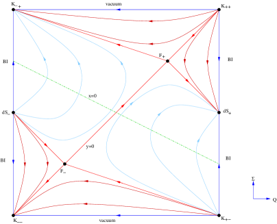
Figure 1: State space R is an invariant submanifold of M that represents general relativity for ${}^{(3)}R\geq 0$. The separatrix $y=Q-\Sigma=0$ precludes bounce behaviour in $Y$ from occurring.

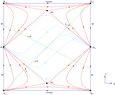
Figure 2: State space M no longer has a separatrix at $y=Q-\Sigma=0$ for $\Omega_{\rho_{*}}>0$. A blue trajectory that passes through the plane $x=Q+2\Sigma=0$ exhibits bounce behaviour in $X$, and a bounce in $Y$ when it passes through the plane $y=Q-\Sigma=0$.

The boundaries $Q=\pm 1$ represent BI models with a cosmological constant, while the boundaries $\Sigma=\pm 1$ correspond to (vacuum) Kasner models in the invariant submanifold

$${\cal R}=\{(Q,\Sigma,\Omega_{\rho_{*}}):|Q|\leq 1,|\Sigma|\leq 1,\Omega_{\rho_{*}}=0\}$$

that represents general relativity. Table 1 contains a list of all critical points, their characterisation and eigenvalues. The points $K_{\pm\pm}$ and $K_{\pm\mp}$ are Kasner solutions that form the vertices of ${\cal R}$. The critical points $K_{++}$ and $K_{+-}$ are repellers, while $K_{--}$ and $K_{-+}$ are attractors. de Sitter spacetime $dS_{+}$ is an attractor and $dS_{-}$ (anti-de Sitter) is a repeller located on the respective boundaries $Q=1$ and $Q=-1$ of the submanifold ${\cal R}$. There are two saddle points $F_{\pm}$ located on the separatrix $y=Q-\Sigma=0$ inside ${\cal R}$. The saddle points $F_{\pm}$ have $\{{}^{(3)}R=2\Lambda,\ \Theta=\sqrt{3}\sigma=\pm\sqrt{\Lambda},\ \rho_{*}=0\}$. From Figure 1 it is clear that no trajectory emerging from $dS_{-}$ inside ${\cal R}$ can to reach $dS_{+}$ due to the separatrix $y=Q-\Sigma=0$. In Figure 2 we demonstrate how the presence of non-local density parameter $\Omega_{\rho_{*}}$ alters the picture. The saddle points $M_{\pm}$ represent static braneworld models with $\{{}^{(3)}R=0,\ \ Theta=0,\ \sigma=\pm\sqrt{2\Lambda},\ \rho_{*}=-3\Lambda\}$. Since $\Omega_{\rho_{*}}=1$ these models are located inside the greater state space

$${\cal M}=\{(Q,\Sigma,\Omega_{\rho_{*}}):|Q|\leq 1,|\Sigma|\leq 1,0\leq\Omega_{\rho_{*}}\leq 1\}$$

but outside ${\cal R}$. A trajectory emerging from $dS_{-}$ may now exit ${\cal R}$ and cross the plane $y=Q-\Sigma=0$ (which is no longer a separatrix for $\Omega_{\rho_{*}}>0$) as it evolves toward, and eventually away from the static models $M_{\pm}$, and enters $dS_{+}$. Such a trajectory passes through $Q=0$ and close to $M_{\pm}$, indicative of bounce behaviour in the volume scale factor $a$, since $Q^{\prime}$ remains positive.

Model	Coordinates	Eigenvalues
$dS_{\pm}$	$(\pm 1,\ 0,\ 0)$	$(\mp 2,\ \mp 3,\ \mp 4)$
$K_{\pm\pm}$	$(\pm 1,\ \pm 1,\ 0)$	$(\pm 2,\ \pm 6,\ \pm 6)$
$K_{\pm\mp}$	$(\pm 1,\ \mp 1,\ 0)$	$(\pm 2,\ \pm 2,\ \pm 6)$
$F_{\pm}$	$(\pm{1\over 2},\ \pm{1\over 2},\ 0)$	$(\pm{3\over 2},\ \mp 2,\ \mp 3)$
$M_{\pm}$	$(0,\ \pm\sqrt{{2\over 3}},\ 1)$	$(\pm 2\sqrt{{2\over 3}},\ 2,\ -2)$

Starting at $dS_{-}$ a trajectory passes through the plane $y=Q-\Sigma=0$, with $y$ changing sign from negative to $0$ to positive, and through the plane $x=Q+2\Sigma=0$ with $x$ changing sign from negative to $0$ to positive. It terminates at the attractor $dS_{+}$. Note that the bounce definition (3.1) requires the trajectory to cut both the $x$- and $y$-planes (the order may be reversed, depending on the path chosen), entering from the negative side of each plane, and exiting the positive side. If it passes through $(0,0,\Omega_{\rho_{*}})$ then the bounce in $X$ and $Y$ is synchronous, i.e. the shear $\sigma$ and the expansion $\Theta$ both vanish there.

6 Conclusion

We have shown that in General Relativity, LRS Bianchi type I, III and Kantowski - Sachs scalar field models that exhibit bounce behaviour violate the reality condition for the momentum density $\dot{\phi}^{2}\geq 0$.

Thus Smolin’s idea of collapse to a black hole state resulting in re - expansion into a new expanding universe region is not viable if the end - state of the universe after collapse into a black hole is described by a Kantowski - Sachs model, even in situations where the matter is dominated by a scalar field.

None of the LRS Bianchi models besides closed FRW and Bianchi IX can support bounce behaviour without significant energy violations. We also analysed this phenomenon in the Randall-Sundrum type braneworld scenario. In this case there are non - local effects transmitted via the bulk Weyl tensor from the gravitational field in the bulk, onto the brane, that makes Kantowski-Sachs brane exhibit bounce behaviour, assuming that the required non - local effects do indeed lead to a physical higher-dimensional bulk (an issue that still remains unresolved [27]). Specifically, a Kantowksi-Sachs brane bounce requires negative non - local energy density if $\sigma_{\mu\nu}\pi_{*}^{\mu\nu}=0$, as demonstrated in section 5.

References

References

- [1] R. C. Tolman, Relativity Thermodynamics and Cosmology (Oxford University Press, 1934; Dover, 1987).
- [2] R. Dicke and P. J. E. Peebles The Big Bang Cosmology: Enigmas and Nostrums. In General relativity, ed. S. W. Hawking and W. Israel (Cambridge University Press, 1979).
- [3] L. Smolin, Did the universe evolve? Class. Qu. Grav. 9, 173 (1992); The Life of the Cosmos (Oxford University Press, 1997).
- [4] D. A. Easson and R. H. Brandenberger, JHEP 0106, 024 (2001).
- [5] S. Carloni, P. K. S. Dunsby, S. Capozziello, A. Troisi Class. Quant. Grav. 22, 4839 (2005),
- [6] A. Raychaudhuri, Phys. Rev. 98, 1123 (1955).
- [7] J. Ehlers, Gen Rel Grav 25, 1225 (1993).
- [8] G. F. R. Ellis, Relativistic Cosmology. In General Relativity and Cosmology, Proc. Int. School of Physics “Enrico Fermi” (Varenna), Course XLVII. ed. R. K. Sachs (Academic Press, 1971), 104-179.
- [9] S. W. Hawking and G. F. R. Ellis, The large-scale structure of space-time, (Cambridge University Press, 1973).
- [10] J. Wainright and G. F. R. Ellis, Dynamical systems in Cosmology, (Cambridge University Press, 1997).
- [11] R. Kantowski and R. K. Sachs, J. Math. Phys. 7, 443 (1967).
- [12] G. F. R. Ellis, J. Math. Phys. 8, 1171 (1967).
- [13] L. Randall and R. Sundrum, Phys. Rev. Lett. 83, 4690 (1999).
- [14] J. Khoury, B. A. Ovrut, P.J. Steinhardt and N. Turok, Phys. Rev. D 64, 123522 (2001); J. Khoury, B.A. Ovrut, N. Seiberg, P.J. Steinhardt and N. Turok, Phys. Rev. D 66, 046005 (2002).
- [15] J. Martin, P. Peter, N. Pinto-Neto and D. J. Schwarz, Phys. Rev. D 65, 123513 (2002); F. Finelli and R. Brandenberger, Phys. Rev. D 65, 103522 (2002); C. Gordon and N. Turok, Phys. Rev. D 67, 123508 (2003); J. Martin, P. Peter, Phys. Rev. D 68, 103517 (2003); L. E. Allen, D. Wands Phys. Rev. D 70, 063515 (2004); G. Geshnizjani, T. J. Battefeld Phys. Rev. D 73, 048501 (2006).
- [16] M. Madsen and G. F. R. Ellis, Class. Quantum Grav. 8, 667 (1991).
- [17] A. V. Toporensky and V. O. Ustiansky Dynamics of Bianchi IX universe with massive scalar field, gr-qc/9907047.
- [18] R. Wald, Phys. Rev. D 28, 2118 (1982).
- [19] C. B. Collins and S.W. Hawking Astrophys. J. 180, 137 (1973); Mon. Not. R. Astr. Soc. 162, 307 (1973).
- [20] P. Horava and E. Witten, Nucl. Phys. B 460, 506 (1996); Nucl. Phys. B 475, 94 (1996).
- [21] Tetsuya Shiromizo, Kei-ichi Maeda and Misao Sasaki, Phys. Rev. D 62, 024012 (2000).
- [22] Andre Lukas, Burt A. Ovrut, KS Stelle and Daniel Waldrum, Phys. Rev. D 59, 086001 (1999).
- [23] R. Maartens, Phys. Rev. D 62, 084023 (2000), hep - th/0004166; Geometry and Dynamics of the Brane - World, in Reference Frames and Gravitomagnetism, ed. J Pascual-Sanchez et al. ,93-119 (World Sci., 2001); gr-qc/0101059.
- [24] A. Campos and C. Sopuerta, Phys. Rev. D 63, 104012 (2001); Phys. Rev. D 64, 104011 (2001).
- [25] N. Goheer and P. K. S. Dunsby, Phys. Rev. D 66, 043527 (2002); Phys. Rev. D 67, 103513 (2003).
- [26] R. Maartens, V. Sahni and T.D. Saini, Phys. Rev. D 63, 063509 (2001); A.V. Toporensky, Class. Quant. Grav. 18, 2311 (2001); M.G. Santos, F. Vernizzi, P.G. Ferreira, Phys. Rev. D, 64,063506 (2001).
- [27] A. Campos, R. Maartens, D. Matravers and C. F. Sopuerta, Phys. Rev D 68, 103520 (2003); A. Fabbri, D. Langlois, D. A. Steer, R. Zegers, JHEP 0409, 025 (2004).