Asymptotic tails of massive scalar fields in Schwarzschild background

Abstract

We investigate the asymptotic tail behavior of massive scalar fields in Schwarzschild background. It is shown that the oscillatory tail of the scalar field has the decay rate of $t^{-5/6}$ at asymptotically late times, and the oscillation with the period $2\pi/m$ for the field mass $m$ is modulated by the long-term phase shift. These behaviors are qualitatively similar to those found in nearly extreme Reissner-Nordström background, which are discussed in terms of a resonant backscattering due to the space-time curvature.

I Introduction

The late-time evolution of various fields outside a collapsing star has important implications for several aspects of black-hole physics. For example, the no-hair theorem [1] introduced by Wheeler in the early 1970’s, states that the external field of a black hole relaxes to a Kerr-Newman field characterized solely by the black-hole’s mass, charge and angular-momentum. Thus, it is of interest to explore the dynamical mechanism responsible for the relaxation of perturbations fields outside a black hole and to determine the decay rate of the various perturbations. In addition, the dynamical mechanism of generating perturbation fields ingoing to a black hole is of interest in relation to the problem of stability of the Cauchy horizon [2].

It was first demonstrated by Price [3], regarding scalar, gravitational and electromagnetic perturbations of Schwarzschild black hole exterior, that the fields die off at late time with an inverse power-law tail. It has been shown that for a spherical-harmonic wave mode of multiple number $l$, a $t^{-2l-2}$ or $t^{-2l-3}$ decay tail ($t$ being the Schwarzschild time coordinate) dominates at late time, depending on the initial conditions. The same tail behavior occurs also for Reissner-Nordström black holes and fields of different spin. Recently the linear perturbation analyses and the nonlinear simulations have been done by Gundlach et al. [4] and [5], respectively. (See also [6].) In addition, the recent treatment of tails in the spacetime of a spinning black hole has been done by Barack and Ori [7].

Many previous works are mainly concerned with massless fields. However, the evolution of massive scalar fields will become important, for example, if one considers Kaluza-Klein theories, in which the Fourier modes can behave like massive fields. Further, the recent development of the Kaluza-Klein idea, such as Rendall-Sundrum model [9] in string theory, strongly motivates us to understand the evolutional features characteristic to the field mass in detail.

The physical mechanism by which late-time tails of massive scalar fields are generated may be qualitatively different from that of massless ones. In fact, it has been pointed out that the oscillatory inverse power-law tails

$$\psi\sim t^{\scriptscriptstyle-l-\frac{3}{2}}\sin(mt),$$ (1)

dominates as the intermediate late-time, if the field mass $m$ is small [10] (see also [11]). It is clear from Eq. (1) that massive fields decay slower than massless ones, and waves with peculiar frequency $\omega$ quite close to $m$ can contribute to massive tail, while low frequency waves can contribute to massless tail. Though the oscillatory power-law form (1) has been numerically verified at intermediate late times, $mM\ll mt\ll 1/(mM)^{2}$, it should be noted that the intermediate tails are not the final asymptotic behaviors; Another wave pattern can dominate at very late times, when it still remains very difficult to determine numerically the exact decay rate [10, 11].

In the previous paper [8], hereafter referred to as paper I, we have analytically found that the transition from the intermediate behavior to the asymptotic one occurs in nearly extreme Reissner-Nordström background. The oscillatory inverse power-law behavior of the dominant asymptotic tail is approximately given by

$$\psi\sim t^{-5/6}\sin(mt),$$ (2)

independently of angular momentum wave number $l$, and the decay becomes slower than the intermediate ones. The origin of such an asymptotic tail is expected to be a resonance backscattering due to curvature-induced potential. This will be supported by the relationship between the field mass and the time scale when the $t^{-5/6}$ tail dominates; For $mM\ll 1$, the smaller $mM$ is, the later the $t^{-5/6}$ tail begins to dominate ($mt\gg 1/(mM)^{2}$, where $M$ is the black-hole mass). On the other hand, for large field mass $mM\gg 1$, the larger $mM$ is, the later the $t^{-5/6}$ tail begins to dominate ($mt\gg mM$). Therefore, the time scale when the $t^{-5/6}$ tail dominates will become minimum at $mM\simeq O(1)$, which means that the most effective backscattering occurs for such massive scalar fields with the Compton wave length $1/m$ nearly equal to the horizon radius $M$.

In this paper, following paper I which was devoted to the analysis for nearly extreme Reissner-Nordström background, we investigate the asymptotic tails of a massive scalar field in Schwarzschild background. The purpose of this paper is to determine analytically the decay rate and to confirm that the asymptotic tail with the decay rate of $t^{-5/6}$ is not peculiar to the nearly extreme black hole. Nevertheless, it is sure that the form of effective potential varies according to the ratio of the black-hole charge to the mass. Then, we also study the difference of the asymptotic tail behavior in Schwarzschild background from that in nearly extreme Reissner-Nordström. In Sec. II, to analyze time evolution of massive scalar fields, we introduce the black-hole Green’s function using the spectral decomposition method [12]. Differently from the case of nearly extreme Reissner-Nordström in paper I, it is difficult to analyze the field equations for the arbitrary field mass $m$. In this paper, therefore, we consider the cases of small field mass $mM\ll 1$ in Sec. III and large one $mM\gg 1$ in Sec. IV, and we compare the results with those found in nearly extreme Reissner-Nordström background. Section V is devoted to a summary.

II Green’s function analysis

A Massive scalar fields in Schwarzschild geometry

We consider time evolution of a massive scalar field in Schwarzschild background with the black-hole mass $M$. The metric is

$$ds^{2}=-\left(1-\frac{2M}{r}\right)dt^{2}+\left(1-\frac{2M}{r}\right)^{-1}dr^{2}+r^{2}d\Omega^{2},$$ (3)

and the scalar field $\phi$ with the mass $m$ satisfies the wave equation

$$(\Box-m^{2})\phi=0.$$ (4)

Resolving the field into spherical harmonics

$$\phi=\sum_{l,m}\frac{\psi^{l}(r)}{r}Y_{lm}(\theta,\varphi),$$ (5)

hereafter we omit the index $l$ of $\psi^{l}$ for simplicity, and we obtain a wave equation for each multiple moment:

$$\psi_{,tt}-\psi_{,r_{\ast}r_{\ast}}+V\psi=0,$$ (6)

where $r_{\ast}$ is the tortoise coordinate defined by

$$dr_{\ast}=\frac{dr}{1-\frac{2M}{r}}\>,$$ (7)

and the effective potential $V$ is

$$V=\left(1-\frac{2M}{r}\right)\left[\frac{l(l+1)}{r^{2}}+\frac{2M}{r^{3}}+m^{2}\right].$$ (8)

B The black-hole Green’s function

The time evolution of a massive scalar field is given by

$$\psi(r_{\ast},t)=\int\left[G(r_{\ast},r_{\ast}^{\prime};t)\psi_{t}(r^{\prime},0)+G_{t}(r_{\ast},r_{\ast}^{\prime};t)\psi(r_{\ast}^{\prime},0)\right]dr_{\ast}^{\prime}$$ (9)

for $t>0$, where the (retarded) Green’s function $G(r,r^{\prime};t)$ is defined as

$$\left[\frac{\partial^{2}}{\partial t^{2}}-\frac{\partial^{2}}{\partial r_{\ast}^{2}}+V\right]G(r_{\ast},r_{\ast}^{\prime};t)=\delta(t)\delta(r_{\ast}-r_{\ast}^{\prime}).$$ (10)

The causality condition gives the initial condition that $G(r,r^{\prime};t)=0$ for $t\leq 0$. In order to find $G(r,r^{\prime};t)$ we use the Fourier transform

$$\tilde{G}(r_{\ast},r^{\prime}_{\ast};\omega)=\int_{0^{-}}^{+\infty}G(r_{\ast},r^{\prime}_{\ast};t)e^{i\omega t}dt.$$ (11)

The Fourier transform is analytic in the upper half $\omega$ plane, and the corresponding inversion formula is

$$G(r_{\ast},r_{\ast}^{\prime};t)=-\frac{1}{2\pi}\int_{-\infty+ic}^{\infty+ic}\tilde{G}(r_{\ast},r^{\prime}_{\ast};\omega)e^{\scriptscriptstyle-i\omega t}d\omega$$ (12)

where $c$ is some positive constant. The usual procedure is to close the contour of integration into the lower half of the complex frequency plane shown in Fig. 1. Then, the late-time tail behaviors which are our main concern should be given by the integral along the branch cut placed along the interval $-m\leq\omega\leq m$.

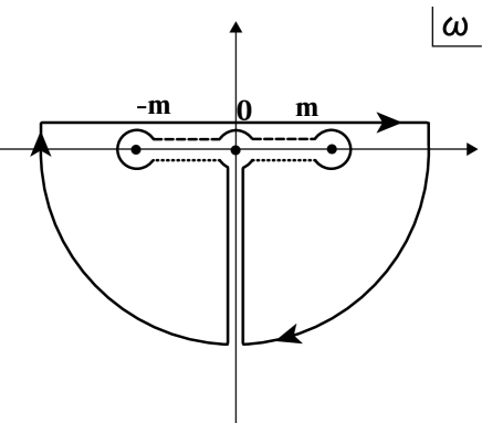
FIG. 1.: Integration contours in the complex frequency plane. The original integration contour for the Green’s function lies above the real frequency axis. We choose the value of $\varpi$ on the dashed line to be $\varpi=|\varpi|$ and that on the dotted lines to be $\varpi=e^{\pm i\pi}|\varpi|$.

Now the Fourier component of the Green’s function $\tilde{G}(r_{\ast},r^{\prime}_{\ast};\omega)$ can be expressed in terms of two linearly independent solutions for the homogeneous equation

$$\left(\frac{d^{2}}{dr_{\ast}^{2}}+\omega^{2}-V\right)\tilde{\psi}_{i}=0\quad i=1,2.$$ (13)

The boundary condition for the basic solution $\tilde{\psi}_{1}$ is that it describes purely ingoing waves crossing the event horizon, i.e.,

$$\tilde{\psi}_{1}\simeq e^{-i\omega r_{\ast}},$$ (14)

at $r_{\ast}\to-\infty$, while $\tilde{\psi}_{2}$ is required to damp exponentially at spatial infinity, i.e.,

$$\tilde{\psi}_{2}\simeq e^{-\varpi r_{\ast}},$$ (15)

at $r_{\ast}\to\infty$, where $\varpi\equiv\sqrt{m^{2}-\omega^{2}}$. Because the complex conjugate $\tilde{\psi}_{1}^{\ast}$ is also a solution for Eq. (13), $\tilde{\psi}_{2}$ can be written by the linear superposition

$$\tilde{\psi}_{2}=\alpha\tilde{\psi}_{1}+\beta\tilde{\psi}_{1}^{\ast},$$ (16)

and the Wronskian is estimated to be

$$W(\omega)=\tilde{\psi}_{1}\tilde{\psi}_{2,r_{\ast}}-\tilde{\psi}_{1,r_{\ast}}\tilde{\psi}_{2}=2i\omega\beta.$$ (17)

Using these two solutions, the Green’s function can be written by

$$\tilde{G}(r_{\ast},r^{\prime}_{\ast};\omega)=-\frac{1}{2i\omega\beta}\left\{\begin{array}[]{l@{\quad,\quad}l}\tilde{\psi}_{1}(r^{\prime}_{\ast},\omega)\tilde{\psi}_{2}(r_{\ast},\omega)&\qquad r^{\prime}_{\ast}>r_{\ast},\\ \tilde{\psi}_{1}(r_{\ast},\omega)\tilde{\psi}_{2}(r^{\prime}_{\ast},\omega)&\qquad r^{\prime}_{\ast}<r_{\ast}.\end{array}\right.$$ (18)

The contribution $G^{C}$ from the branch cut to the Green’s function is reduced to

$$G^{C}(r_{\ast},r_{\ast}^{\prime};t) = -\frac{1}{4\pi i}\int_{\rm{cut}}\frac{1}{\omega}\frac{\alpha}{\beta}\tilde{\psi}_{1}(r_{\ast}^{\prime},\omega)\tilde{\psi}_{1}(r_{\ast},\omega)e^{-i\omega t}d\omega.$$ (19)

Then the main task to evaluate $G^{C}$ is to derive the coefficients $\alpha$ and $\beta$.

C Effective contributions to tail behaviors

Here we point out the at very late times $mt\gg 1$ the rapidly oscillating term $e^{-i\omega t}$ leads to a mutual cancellation between the positive and the negative parts of the integrand in Eq.(19). Then, the effective contribution to the tail behaviors arises from the narrow range

$$\epsilon\equiv 2M\varpi\ll 1,$$ (20)

which was also claimed in [10, 14].

III small-mass case

Introducing the non-dimensional variable defined as

$$x \equiv \frac{r}{2M},$$ (21)

Eq.(13) is rewritten by

$$\frac{d^{2}\tilde{\psi}}{dx^{2}}+\frac{1}{x(x-1)}\frac{d\tilde{\psi}}{dx}+\Bigg{[}\frac{4M^{2}\omega^{2}x^{2}}{(x-1)^{2}}-\frac{4M^{2}m^{2}x}{x-1}-\frac{l(l+1)}{x(x-1)}-\frac{1}{x^{2}(x-1)}\Bigg{]}\tilde{\psi}=0.$$ (22)

To study analytically the mode solutions $\psi$, the asymptotic matching between the inner and outer solutions was successfully used in paper I for the potential $V$ in nearly extreme Reissner-Nordström background. However, to apply the same method to Eq.(22), it is necessary to assume the field mass to be very small or very large. In this section we consider the small-mass case $mM\ll 1$.

A Mode solutions

1 The inner region $1\leq x\ll 1/m^{2}M^{2}$

For the small-mass case such as $mM\ll 1$, truncating the terms of the order $m^{2}M^{2}$, we can approximate Eq.(22) by

$$\frac{d^{2}\tilde{\psi}}{dx^{2}}+\left(\frac{1}{x-1}-\frac{1}{x}\right)\frac{d\tilde{\psi}}{dx}+\Bigg{[}\frac{4M^{2}m^{2}}{(x-1)^{2}}+\frac{4M^{2}m^{2}-l^{2}-l-1}{x(x-1)}+\frac{1}{x^{2}}\Bigg{]}\tilde{\psi} = 0.$$ (23)

Now the solution $\psi_{1}$ satisfying the boundary condition (14) can be written using the hyper-geometric function $F$ as follows,

$$\psi_{1} = x^{K_{++}}(x-1)^{-2iMm}F\left(K_{--},K_{--};1-4iMm;1-\frac{1}{x}\right)$$ (24)

$$= x^{K_{++}}(x-1)^{-2iMm}\frac{\Gamma(1-4iMm)\Gamma(2\mu)}{\Gamma(K_{+-})^{2}}F\left(K_{--},K_{--};1-2\mu;\frac{1}{x}\right)$$ (26)

$$+x^{K_{-+}}(x-1)^{-2iMm}\frac{\Gamma(1-4iMm)\Gamma(-2\mu)}{\Gamma(K_{--})^{2}}F\left(K_{+-},K_{+-};1+2\mu;\frac{1}{x}\right),$$

where $\mu$ and $K_{\pm\pm}$ are

$$\mu = \sqrt{\left(l+\frac{1}{2}\right)^{2}-8M^{2}m^{2}}$$ (27)

and

$$K_{\pm\pm} = \frac{1}{2}\pm\mu\pm 2iMm,$$ (28)

respectively. and we used the linear transformation formulas (15.3.6) of [13] in the second equality of Eq. (24). If estimated in the region $x\gg 1$, we obtain

$$\tilde{\psi}_{1} \to \frac{\Gamma(1-4iMm)\Gamma(2\mu)}{\Gamma(K_{+-})^{2}}x^{\mu+\frac{1}{2}}+\frac{\Gamma(1-4iMm)\Gamma(-2\mu)}{\Gamma(K_{--})^{2}}x^{-\mu+\frac{1}{2}},$$ (29)

which is necessary for asymptotic matching in the overlap region $1\ll x\ll 1/(mM)^{2}$ with the outer solutions valid in the region $x\gg 1$.

2 The outer region $x\gg 1$

For large $x$, Eq.(22) is approximated by

$$\frac{d^{2}\tilde{\psi}}{dx^{2}}+\Bigg{[}\frac{4M^{2}m^{2}}{x}-\epsilon^{2}+\frac{8M^{2}m^{2}-l(l+1)}{x^{2}}\Bigg{]}\tilde{\psi} = 0.$$ (30)

Then we can write the solutions using Whittaker’s functions. The mode solution $\psi_{2}$ satisfying the boundary condition (15) should be

$$\psi_{2} = W_{\sigma,\mu}(2\epsilon x),$$ (31)

where

$$\sigma = \frac{2M^{2}m^{2}}{\epsilon}-\epsilon.$$ (32)

If estimated in the region $x\ll 1/\epsilon$, we obtain

$$\tilde{\psi}_{2} \to \frac{\Gamma(-2\mu)}{\Gamma(\frac{1}{2}-\mu-\sigma)}(2\epsilon)^{\mu+\frac{1}{2}}x^{\mu+\frac{1}{2}}+\frac{\Gamma(2\mu)}{\Gamma(\frac{1}{2}+\mu-\sigma)}(2\epsilon)^{-\mu+\frac{1}{2}}x^{-\mu+\frac{1}{2}}.$$ (33)

3 Matching

We can match the solution (29) valid at $1\ll x\ll 1/m^{2}M^{2}$ with the solution (33) valid at $1\ll x\ll 1/\epsilon$ in the overlap region and determine the coefficients $\alpha$ and $\beta$ in Eq.(19). Then the ratio is given as follows,

$$\frac{\alpha}{\beta}(|\omega|,\epsilon)\Bigg{|}_{|\omega|\to m} = \Bigg{[}-(2\epsilon)^{\mu+\frac{1}{2}}\frac{\Gamma(-2\mu)^{2}\Gamma(1+4iMm)}{\Gamma(\frac{1}{2}-\mu-\sigma)\Gamma(K_{-+})^{2}}$$ (35)

$$+(2\epsilon)^{-\mu+\frac{1}{2}}\frac{\Gamma(2\mu)^{2}\Gamma(1+4iMm)}{\Gamma(\frac{1}{2}+\mu-\sigma)\Gamma(K_{++})^{2}}\Bigg{]}\times({\rm complex\>conjugate})^{-1}.$$

B Intermediate tails

The effective contribution to the integral in Eq. (19) is claimed to be limited to the range $|\omega-m|=O(1/t)$ or equivalently $\varpi=O(\sqrt{m/t})$, since the rapidly oscillating term $e^{-i\omega t}$ which leads to a mutual cancellation between the positive and the negative parts of the integrand (see [10, 8]). The intermediate tails becomes dominant at the late times in the range

$$mM\ll mt\ll\frac{1}{(mM)^{2}},$$ (36)

when the integral (19) should be estimated under the condition

$$\sigma\simeq\frac{2m^{2}M^{2}}{\epsilon}=O(mM\sqrt{mt})\ll 1.$$ (37)

As was discussed in paper I, the small value of $\sigma$ represents that the backscattering due to the spacetime curvature is not effective at intermediate late times. Then, using the condition (37), we obtain

$$\frac{\alpha}{\beta}(|\omega|,\epsilon)-\frac{\alpha}{\beta}(|\omega|,e^{-i\pi}\epsilon)\Bigg{|}_{|\omega|\to m}\sim i\frac{2^{2l+1}l!^{6}}{(2l)!^{2}(2l+1)!^{4}}mM\epsilon^{2l+1},$$ (38)

which is identical with Eq. (51) in paper I. Therefore, it is obvious that the same intermediate tails as Eq. (1) dominate at intermediate late times (36), which was numerically supported by [10, 11].

C Asymptotic tails

As discussed in paper I, the intermediate tails can not be an asymptotic behavior, and the long-term evolution from the intermediate behavior to the final one should occur. The asymptotic tail becomes dominant at very late times such that

$$mt\gg\frac{1}{m^{2}M^{2}},$$ (39)

when the effective contribution to the integral (19) arises from the region

$$\sigma\simeq\frac{2m^{2}M^{2}}{\epsilon}\gg 1,$$ (40)

which means backscattering effect due to curvature-induced potential dominates. Then, the ratio of $\alpha$ to $\beta$ is approximately given by

$$\frac{\alpha}{\beta}(|\omega|,\epsilon)\Bigg{|}_{|\omega|\to m} \to \frac{\eta^{\ast}e^{i\pi\sigma}+\gamma^{\ast}e^{-i\pi\sigma}}{\eta e^{-i\pi\sigma}+\gamma e^{i\pi\sigma}},$$ (41)

where

$$\eta = -\frac{\Gamma(-2\mu)^{2}\Gamma(1-4iMm)}{\Gamma(K_{--})^{2}}(4m^{2}M^{2})^{\mu}e^{-i\pi\mu}+\frac{\Gamma(2\mu)^{2}\Gamma(1-4iMm)}{\Gamma(K_{+-})^{2}}(4m^{2}M^{2})^{-\mu}e^{i\pi\mu},$$ (42)

and

$$\gamma = -\frac{\Gamma(-2\mu)^{2}\Gamma(1-4iMm)}{\Gamma(K_{--})^{2}}(4m^{2}M^{2})^{\mu}e^{i\pi\mu}+\frac{\Gamma(2\mu)^{2}\Gamma(1-4iMm)}{\Gamma(K_{+-})^{2}}(4m^{2}M^{2})^{-\mu}e^{-i\pi\mu}.$$ (43)

As was shown in the paper I, the contribution from the Green’s function to the asymptotic tail part corresponds to the integral along the dashed line in Fig. 1 which is approximated by

$$G^{C}(r_{\ast},r_{\ast}^{\prime};t) \simeq \frac{1}{4\pi mi}\tilde{\psi}_{1}(r_{\ast},m)\tilde{\psi}_{1}(r^{\prime}_{\ast},m)\int_{\rm dashed\>line}e^{i(2\pi\sigma-\omega t)}e^{i\varphi_{s}}d\omega+({\rm complex\>conjugate}),$$ (44)

where the phase $\varphi_{s}$ is defined by

$$e^{i\varphi_{s}}=\frac{\eta^{\ast}+\gamma^{\ast}e^{-2i\pi\sigma}}{\eta+\gamma e^{2i\pi\sigma}},$$ (45)

and it remains in the range $0\leq\varphi_{s}\leq 2\pi$, even if $\sigma$ becomes very large, since we have

$$|\eta|^{2}-|\gamma|^{2} = \frac{2\pi Mm}{\mu}\>>\>0.$$ (46)

Because the terms $e^{-i\omega t}$ and $e^{2i\pi\sigma}$ in Eq.(44) are rapidly oscillating at very late times, the saddle-point integration allows us to evaluate accurately the asymptotic behaviors. Let us introduce the variable $a$ defined by

$$a\equiv\left(1-\frac{\omega}{m}\right)^{1/2}(mt)^{1/3}.$$ (47)

Then, the oscillation terms $e^{i(2\pi\sigma-\omega t)}$ in Eq.(44) can be approximately rewritten into the form

$$e^{i(mt)^{1/3}f_{s}(a)}e^{-imt}$$ (48)

in the limits $mt\to\infty$ and $\omega/m\to 1$, by keeping $a$ to be finite. Here we have

$$f_{s}(a)=\frac{\sqrt{2}\pi mM}{a}+a^{2}.$$ (49)

The saddle point is found to exist at

$$a=a_{0}\equiv\left(\frac{\pi mM}{\sqrt{2}}\right)^{1/3}.$$ (50)

At the saddle point the parameter $\epsilon$ defined by Eq.(20) is given by

$$\epsilon_{0}\equiv 2M\sqrt{m^{2}-\omega_{0}^{2}}\simeq 2\left(\frac{2\pi}{mt}\right)^{1/3}(mM)^{4/3},$$ (51)

or equivalently

$$\sigma_{0}\simeq mM\left(\frac{2\pi mM}{mt}\right)^{1/3}$$ (52)

which is equal to the value obtained in the nearly extreme case in paper I. Let us give the Taylor expansion of $f$ near the point $a=a_{0}$ as follows,

$$f_{s}(a) \simeq f_{s}(a_{0})+\frac{1}{2}(a-a_{0})^{2}f_{s}^{\prime\prime}(a_{0})$$ (53)

$$= 3\left(\frac{\pi mM}{\sqrt{2}}\right)^{2/3}+3(a-a_{0})^{2}.$$ (54)

Then, the integral in Eq.(44) can be approximately estimated to be

$$G^{C}(r_{\ast},r^{\prime}_{\ast};t) \simeq \frac{1}{2\sqrt{3}}(2\pi)^{\frac{5}{6}}(mM)^{\frac{1}{3}}(mt)^{-\frac{5}{6}}\sin(mt-3(2\pi mM)^{2/3}(mt)^{1/3}/2-\varphi_{s}(\sigma_{0})+3\pi/4)$$ (56)

$$\times\tilde{\psi}_{1}(r_{\ast},m)\tilde{\psi}_{1}(r_{\ast}^{\prime},m),$$

at very late times $mt\gg 1/(mM)^{2}$. The oscillation has the period $2\pi/m$, and is modulated by the two types of long-term phase shifts. First, the term $(3/2)(2\pi mM)^{2/3}(mt)^{1/3}$ represents a monotonously increasing phase shift. Second, the term $\varphi_{s}(\sigma_{0})$ represents a periodic phase shift with the amplitude $|\varphi_{s}|$ smaller than $2\pi$, which will be studied in the following. Eq.(56) is similar to Eq.(69) in paper I, though the corresponding terms of the phase shift are omitted in Eq.(69) in paper I since we have focused our attention to the decay rate.

D Phase shift

Now we study the periodic phase-shift effect caused by the term $\varphi_{s}(\omega_{0})$. From the equation

$$\frac{d\varphi_{s}}{d\sigma} = 0,$$ (57)

we find the maximum and minimum extremes, denoted by $\varphi_{s+}(\sigma_{+})$ and $\varphi_{s-}(\sigma_{-})$ of $\varphi_{s}$ at $\sigma=\sigma_{+}$ and $\sigma=\sigma_{-}$, which given by

$$\varphi_{s\pm}(\sigma_{\pm}) = \pm 2\theta+\varphi_{s0},$$ (58)

and

$$2\pi\sigma_{\pm} = \pi\mp\frac{\pi}{2}\pm\theta+const,$$ (59)

where

$$\sin\theta = \left|\frac{\gamma}{\eta}\right|$$ (60)

and

$$\exp(i\varphi_{s0})\equiv\frac{\eta^{\ast}}{\eta}.$$ (61)

Expanding $|\gamma/\eta|$ with respect to $mM\ll 1$, we obtain

$$\left|\frac{\gamma}{\eta}\right| = 1-\delta,$$ (62)

and

$$\delta \simeq \pi\left(\frac{64}{15}\right)^{2}(mM)^{3}\qquad({\rm for}\>l=0),$$ (63)

$$\simeq \frac{2^{4l+4}\pi(l!)^{4}}{(2l+1)(2l)!^{4}}(mM)^{4l+3}\qquad({\rm for}\>l\geq 0)$$ (64)

in Schwarzschild background. The phase-shift term $\delta$ is characteristic to the black hole. For example, for nearly extreme Reissner-Nordström background [8], the value of $\delta$ is given by

$$\delta_{\rm nearly\>extreme} \simeq \pi\left(\frac{50}{23}\right)^{2}(mM)^{3}\qquad({\rm for}\>l=0),$$ (65)

$$\simeq \frac{2^{4l+3}\pi(l!)^{2}}{(2l+1)^{2}(2l)!^{4}}(mM)^{6l+3}\qquad({\rm for}\>l\geq 0).$$ (66)

From Eqs. (58) and (59) the oscillation amplitude of $\varphi_{s}$ is given by

$$\Delta\varphi_{s} \equiv \varphi_{s+}-\varphi_{s-}=4\theta$$ (67)

$$\simeq 2\pi-\sqrt{2\delta},$$ (68)

and the time interval between the two extremes is estimated to be

$$2\pi\Delta\sigma \equiv 2\pi(\sigma_{-}-\sigma_{+})=\pi-2\theta$$ (69)

$$\simeq \sqrt{8\delta}.$$ (70)

These equations mean that the smaller the field mass is, the more rapidly the change of the phase $\varphi_{s}$ from the maxixum to the minimum occurs (see Fig. 2). The phase shift oscillates at the time scale of $1/(m^{3}M^{2})$, which is much longer than the period of $2\pi/m$. So it is a long-term effect which modulates the basic oscillation.

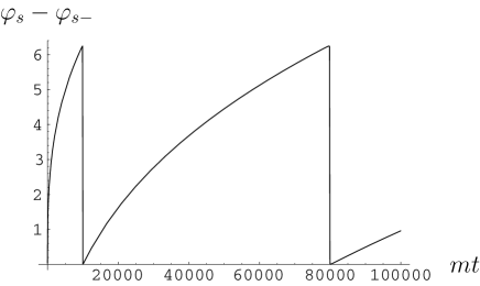
FIG. 2.: Time evolution of the phase $\varphi_{s}-\varphi_{s-}$ in the case of $mM=0.01$ and $l=0$.

IV large mass case

A Mode solutions

In this section we consider large-mass case such as $mM\gg 1$. It is enough to consider the narrow region (20) in the same manner with the small-mass case. Introducing the function $\xi$ defined as

$$\tilde{\psi}=\sqrt{\frac{r}{r-2M}}\xi=\sqrt{\frac{x}{x-1}}\xi,$$ (71)

the mode equation (22) can be approximately given by

$$\frac{d^{2}\xi^{2}}{dx^{2}}+\Bigg{[}\frac{4M^{2}\omega^{2}x^{2}}{(x-1)^{2}}-\frac{4M^{2}m^{2}x}{x-1}\Bigg{]}\xi = 0,$$ (72)

since the other terms become negligibly small all over the region $x\geq 1$ in comparison with the two terms in the potential. Then we can write solutions for Eq.(72) using Whittaker’s functions. The solutions $\psi_{1}$ and $\psi_{2}$ satisfying the boundary condition (14) and (15), respectively, are

$$\tilde{\psi}_{1} = \sqrt{\frac{x}{x-1}}M_{\sigma,\rho}\left(2\epsilon(x-1)\right),$$ (73)

and

$$\tilde{\psi_{2}} = \sqrt{\frac{x}{x-1}}W_{\sigma,\rho}\left(2\epsilon(x-1)\right),$$ (74)

where

$$\rho = -i\sqrt{4M^{2}\omega^{2}-\frac{1}{4}}.$$ (75)

From Eqs. (73) and (74), $\psi_{2}$ can be rewritten as

$$\tilde{\psi}_{2}=\frac{\Gamma(-2\rho)}{\Gamma(\frac{1}{2}-\rho-\sigma)}\psi_{1}+\frac{\Gamma(2\rho)}{\Gamma(\frac{1}{2}+\rho-\sigma)}\psi_{1}^{\ast}$$ (76)

and the ratio of $\alpha$ to $\beta$ in Eq.(16) is

$$\frac{\alpha}{\beta} = \frac{\Gamma(-2\rho)\Gamma(\frac{1}{2}+\rho-\sigma)}{\Gamma(2\rho)\Gamma(\frac{1}{2}-\rho-\sigma)}.$$ (77)

B Asymptotic tail

As was discussed in paper I, no intermediate tails appear for the scalar field with large mass, namely $mM\gg 1$. At late times given by Eq.(40), the ratio of $\alpha$ to $\beta$ is approximately written by

$$\frac{\alpha}{\beta}(|\omega|,\epsilon)\Bigg{|}_{|\omega|\to m} \to \frac{\zeta^{\ast}e^{i\pi\sigma}-\chi^{\ast}e^{-i\pi\sigma}}{\zeta e^{-i\pi\sigma}-\chi e^{i\pi\sigma}}\epsilon^{-2\rho},$$ (78)

where

$$\zeta = \Gamma(2\rho)(2m^{2}M^{2})^{-\rho}e^{i\pi\rho},$$ (79)

and

$$\chi = \Gamma(2\rho)(2m^{2}M^{2})^{-\rho}e^{-i\pi\rho}.$$ (80)

Substituting Eq.(78) into Eq.(19), we obtain the contribution from Green’s function to the asymptotic tail;

$$G^{C}(r_{\ast},r_{\ast}^{\prime};t) \simeq \frac{1}{4\pi mi}\tilde{\psi}_{1}(r_{\ast},m)\tilde{\psi}_{1}(r^{\prime}_{\ast},m)\int_{\rm dashed\>line}e^{2i\pi\sigma-2\rho\ln\epsilon-i\omega t}e^{i\varphi_{l}}d\omega+({\rm complex\>conjugate}),$$ (81)

where the phase $\varphi_{l}$ is defined by

$$e^{i\varphi_{l}}=\frac{\zeta^{\ast}+\chi^{\ast}e^{-2i\pi\sigma}}{\zeta+\chi e^{2i\pi\sigma}},$$ (82)

and it remains in the range $0\leq\varphi_{l}\leq 2\pi$, even if $\sigma$ becomes very large, since we have

$$|\zeta|^{2}-|\chi|^{2} = \Gamma(2\rho)\Gamma(-2\rho)\left(e^{2i\pi\rho}-e^{-2i\pi\rho}\right)\>>\>0.$$ (83)

Because the terms $e^{-i\omega t}$, $e^{2i\pi\sigma}$ and $e^{-2\rho\ln\epsilon}$ in Eq.(81) are rapidly oscillating at very late times, the saddle-point integration allows us to evaluate accurately the asymptotic behaviors. Just like the small-mass case in the previous section, using the parameter $a$ defined as Eq. (47), the oscillation terms $e^{i(2\pi\sigma-\omega t-2\rho\ln\epsilon)}$ in Eq.(44) can be rewritten into the form

$$e^{i(mt)^{1/3}f_{l}(a)}e^{-imt}$$ (84)

in the limits $mt\to\infty$ and $\omega/m\to 1$, by keeping $a$ to be finite. Here we have

$$f_{l}(a)\simeq\frac{\sqrt{2}\pi mM}{a}+a^{2}+\frac{4mM}{(mt)^{1/3}}\ln\left[\frac{2\sqrt{2}mMa}{(mt)^{1/3}}\right].$$ (85)

The saddle point can be approximated by

$$a_{0} \simeq \left(\frac{\pi mM}{\sqrt{2}}\right)^{1/3}$$ (86)

for asymptotically late times

$$mt\gg mM.$$ (87)

Note that Eq. (86) is identical with Eq. (50). Evaluating Eq. (81) using the saddle point integration, we obtain the asymptotic tail behavior

$$G^{C}(r_{\ast},r^{\prime}_{\ast};t) \simeq \frac{1}{2\sqrt{3}}(2\pi)^{\frac{5}{6}}(mM)^{\frac{1}{3}}(mt)^{-\frac{5}{6}}$$ (90)

$$\times\sin(mt-3/2(2\pi mM)^{2/3}(mt)^{1/3}-4mM\ln\epsilon_{0}-\varphi_{l}(\sigma_{0})+3\pi/4)$$

$$\times\tilde{\psi}_{1}(r_{\ast},m)\tilde{\psi}_{1}(r_{\ast}^{\prime},m).$$

The additional relation (87) is necessary for the asymptotic tail (90) to dominate. The oscillation has the period $m/2\pi$ and is modulated by the two types of phase shifts. First, the terms $(3/2)(2\pi mM)^{2/3}(mt)^{1/3}+4mM\ln\epsilon_{0}$ represent a monotonous phase shift. Second, the term $\varphi_{l}(\sigma_{0})$ represents a periodic phase shift since it remains within $0\leq\varphi_{l}\leq 2\pi$. The decay rate of the asymptotic tail in Schwarzschild background is $t^{-5/6}$, which remains identical with that in nearly extreme Reissner-Nordström background shown in the paper I.

C Phase shift

In the same manner with the small mass case, we study the periodic phase-shift effect which is caused by the term $e^{i\varphi_{l}}$ in Eq.(82). In the large mass limit $mM\gg 1$, the ratio of $\chi$ and $\zeta$ is approximated by

$$\left|\frac{\chi}{\zeta}\right| \simeq e^{-\pi 4mM}\ll 1$$ (91)

in the Schwarzschild case. On the other hand, in the nearly extreme Reissner-Nordström limit, we obtain the large mass limit from Eqs.(59) and (60) in paper I as follows,

$$\left|\frac{\chi}{\zeta}\right|_{\rm nearly\>extreme} \simeq e^{-\pi\sqrt{5}mM}\ll 1.$$ (92)

The oscillation amplitude $\Delta\varphi_{l}$ of $\varphi_{l}$ is

$$\Delta\varphi_{l} \simeq 4\left|\frac{\chi}{\zeta}\right|,$$ (93)

for which Eqs. (91) and (92) give different values, though it remains same that $\Delta\varphi$ vanishes in the large-mass limit.

V Summary

In this paper we have investigated asymptotic tail behaviors of massive scalar fields in Schwarzschild background. We have shown that the asymptotic oscillatory tail with the decay rate of $t^{-5/6}$ and with the period $2\pi/m$ dominates, which is identical with that in nearly extreme Reissner-Nordström background. In addition, we have noted that the relation between the value of $mM$ and the time-scale when the $t^{-5/6}$ tail begins to dominate also holds; The smaller the value of $mM$ is, the later the $t^{-5/6}$ tail begins to dominate ($mt\gg 1/(mM)^{2}$). The larger the value of $mM$ is, the later the $t^{-5/6}$ tail begins to dominate ($mt\gg mM$).

As far as the intermediate late-time behavior is concerned, our result agrees with [10]. However they claimed ”SI perturbation fields decay at late times slower than any power law” in [10], which disagree with the expressions (56) and (81). We believe that their simulation was not carried out until enough late times for the asymptotic tail to dominate or there occured numerical errors in their simulation. Also, our result is consistent with [11], which was done numerically (both for a test field and for the fully nonlinear cases).

In terms of the phase shift we can understand more clearly the tail behavior to be a backscattering effect due to space-time curvature. In the small-mass case $mM\ll 1$, the intermediate tail with an oscillatory power-law dominates at the time scale $1\ll mt\ll 1/(mM)^{2}$ before the asymptotic tail discussed here dominates [8, 10] (see also [11]). At both the intermediate and asymptotic time scales the frequency of a wave which contributes to tails is very close to $m$. However, the oscillation of the asymptotic tail is modulated by phase shift effects which do not appear in the intermediate tail. There exist two types of the phase shift, which are monotonous and periodic with time. The periodic phase shift crucially depends on the field mass. The shift angle becomes nearly equal to $2\pi$ in small mass limit $mM\to 0$, and the shift oscillates at the time scale of $1/(m^{3}M^{2})$, which is a long-term effect if compared with the basic oscillation with the period of $2\pi/m$. In large mass limit $mM\to\infty$, the shift angle become very small. In scattering theory, it is well-known that the phase shift of wave is connected with the presence of the scatterer. In this case, of course, the scatterer is the effective potential of black-hole spacetime. Therefore it is clear that tails of massive scalar fields are generated from backscattering due to space-time curvature. The shift angle in Schwarzschild geometry is numerically different from that in nearly extreme Reissner-Nordström geometry, but the qualitative behavior depending on $mM$ is similar.

We can conclude that the asymptotic tail with the qualitatively same behavior dominates both in Schwarzschild and in nearly extreme Reissner-Nordström background. Therefore it is conjectured that the oscillatory $t^{-5/6}$ tail caused by resonance backscattering at asymptotic late times is a general feature in arbitrary Reissner-Nordström background. It remains in a future work to investigate what kind of instability of Cauchy horizons is caused by the massive tails.

Finally we give a comment in comparison with the effects induced by the field mass $m$ on vacuum polarization of quantum massive scalar fields in the thermal state. It has been found that the amplitude of vacuum polarization is enhanced around $mM\simeq O(1)$ in the case of nearly extreme Reissner-Nordström geometry, while it is not seen in Schwarzschild case [14]. The field-mass induced effect on vacuum polarization becomes clear only in the nearly extreme limit. The reason will be explained as follows; Vacuum polarization of massive scalar fields is due to both thermal excitation induced by black-hole temperature and mass induced excitation. In nearly extreme case, of which the black-hole temperature is nearly zero, the mass induced effect becomes significant because the thermal excitation is suppressed. On the other hand, in Schwarzschild case the mass induced effect is just hidden because the thermal effect by the black-hole temperature can dominate.

We expect that resonance behavior due to the mass of a field interacting with a black hole may exist in various processes as a generic feature of black-hole geometry. In order to confirm this conjecture, it is necessary to investigate various processes of massive fields in more general black hole models. This will be one of the interesting subjects in black-hole physics.

REFERENCES

• [1] R. Ruffini and J. A. Wheeler, Phys. Today 24, 30 (1971), C. W. Misner, K. S. Thone, and J. A. Wheeler, Gravitation (Freeman, San Francisco, 1973).
• [2] E. Poisson and W. Israel, Phys. Rev. D 41, 1796 (1990).
• [3] R. H. Price, Phys. Rev. D 5, 2419 (1972).
• [4] C. Gundlach, R. H. Price, and J. Pullin, Phys. Rev. D 49, 883 (1994).
• [5] C. Gundlach, R. H. Price, and J. Pullin, Phys. Rev. D 49, 890 (1994).
• [6] L. M. Burko and A. Ori, Phys.Rev. D 56,7820 (1997).
• [7] L. Barack and A. Ori, Phys.Rev.Lett. 82, 4388 (1999).
• [8] H. Koyama and A. Tomimatsu, Phys. Rev. D 63, 064032 (2001).
• [9] L. Randall and R. Sundrum, Phys. Rev. Lett. 83, 4690 (1999).
• [10] S. Hod and T. Piran, Phys. Rev. D 58, 044018 (1998).
• [11] L. M. Burko, in Abstracts of plenary talks and contributed papers of the 15th International Conference on General Relativity and Gravitation, Pune, 1997, p. 143 (unpublished).
• [12] E. W. Leaver, Phys. Rev. D 34, 384 (1986).
• [13] Handbook of Mathematical Functions, edited by M. Abramowitz and I.A. Stegun (Dover, New York, 1970).
• [14] A. Tomimatsu and H. Koyama, Phys. Rev. D 61, 124010 (2000).