Exact relativistic treatment of stationary counter-rotating dust disks I
Boundary value problems and solutions

Abstract

This is the first in a series of papers on the construction of explicit solutions to the stationary axisymmetric Einstein equations which describe counter-rotating disks of dust. These disks can serve as models for certain galaxies and accretion disks in astrophysics. We review the Newtonian theory for disks using Riemann-Hilbert methods which can be extended to some extent to the relativistic case where they lead to modular functions on Riemann surfaces. In the case of compact surfaces these are Korotkin’s finite gap solutions which we will discuss in this paper. On the axis we establish for general genus relations between the metric functions and hence the multipoles which are enforced by the underlying hyperelliptic Riemann surface. Generalizing these results to the whole spacetime we are able in principle to study the classes of boundary value problems which can be solved on a given Riemann surface. We investigate the cases of genus 1 and 2 of the Riemann surface in detail and construct the explicit solution for a family of disks with constant angular velocity and constant relative energy density which was announced in a previous Physical Review Letter.

PACS numbers: O4.20.Jb, 02.10.Rn, 02.30.Jr

1 Introduction

The importance of stationary axisymmetric spacetimes arises from the fact that they can describe stars and galaxies in thermodynamical equilibrium (see e.g. [1, 2]). However the complicated structure of the Einstein equations in the matter region which are apparently not completely integrable has made a general treatment of these equations impossible up to now. Thus only special, possibly unphysical solutions like the one of Wahlquist [3] were found (in [4] it was shown that the Wahlquist solution cannot be the interior solution for a slowly rotating star). Since the vacuum equations in the form of Ernst [5] are known to be completely integrable [6, 7, 8], the study of two-dimensional matter models can lead to global solutions of the Einstein equations which hold both in the matter and in the vacuum region: the equations in the matter, which is in general approximated as an ideal fluid, reduce to ordinary non-linear differential equations because one of the spatial dimensions is suppressed. The matter thus leads to boundary values for the vacuum equations.

Disks of pressureless matter, so-called dust, are studied in astrophysics as models for certain galaxies and for accretion disks. We will therefore discuss dust disks in more detail, but the used techniques can in principle be extended to more general cases. In the context of galaxy models, relativistic effects only play an important role in the presence of black-holes since the latter are genuinely relativistic objects. A complete understanding of the black-hole disk system even in non-active galaxies is therefore merely possible in a relativistic setting. The precondition to construct exact solutions for stationary black-hole disk systems is the ability to treat relativistic disks explicitly. In this article we will focus on disks of pressureless matter. By constructing explicit solutions, we hope to get a better understanding of the mathematical structure of the field equations and the physics of rapidly rotating relativistic bodies since dust disks can be viewed as a limiting case for extended matter sources. Hence we will discuss relativistic effects for models whose Newtonian limit is of astrophysical importance. We will investigate disks with counter-rotating dust streams which are discussed as models for certain $S0$ and $Sa$ galaxies (see [9] and references given therein and [10, 11]). These galaxies show counter-rotating matter components and are believed to be the consequence of the merger of galaxies. Recent investigations have shown that there is a large number of galaxies (see [9], the first was NGC 4550 in Virgo) which show counter-rotating streams in the disk with up to 50 % counter-rotation.

Exact solutions describing relativistic disks are also of interest in the context of numerics. They can be used to test existing codes for stationary axisymmetric stars as in [12, 13]. Since Newtonian dust disks are known to be unstable against fragmentation and since numerical investigations (see e.g. [14]) indicate that the same holds in the relativistic case, such solutions could be taken as exact initial data for numerical collapse calculations: due to the inevitable numerical error such an unstable object will collapse if used as initial data.

In the Newtonian case, dust disks can be treated in full generality (see e.g. [15]) since the disks lead to boundary value problems for the Laplace equations which can be solved explicitly. The fact that the complex Ernst equation which takes the role of the Laplace equation in the relativistic case is completely integrable gives rise to the hope that boundary value problems might be solvable here at least in selected cases. The unifying framework for both the Laplace and the Ernst equation is provided by methods from soliton theory, so-called Riemann-Hilbert problems: the scalar problem for the Laplace equation can be always solved with the help of a generalization of the Cauchy integral (see [16] and references given therein), a procedure which leads to the Poisson integral for distributional densities. Choosing the contour of the Riemann-Hilbert problem appropriately one can construct solutions to the Laplace equation which are everywhere regular except at a disk where the function is not differentiable. Similarly one can treat the relativistic case where the matrix Riemann-Hilbert problem can be related to a linear integral equation. It was shown in [17] that the matrix problem for the Ernst equation can be always gauge transformed to a scalar problem on a Riemann surface which can be solved explicitly in terms of Korotkin’s finite gap solutions [18] for rational Riemann-Hilbert data. In this sense these solutions can be viewed as a generalization of the Poisson integral to the relativistic case.

Whereas the Poisson integral contains one free function which is sufficient to solve boundary value problems for the scalar gravitational potential, the finite gap solutions contain one free function and a set of complex parameters, the branch points of the Riemann surface. Thus one cannot hope to solve general boundary value problems for the complex Ernst potential within this class because this would imply the choice to specify two free functions in the solution according to the boundary data. This means that one can only solve certain classes of boundary value problems on a given compact Riemann surface. In the first article we investigate the implications of the underlying Riemann surface on the multipole moments and the boundary values taken at a given boundary. The relations will be given for general genus of the surface and will be discussed in detail in the case of genus 1 (elliptic surface) and genus 2, which is the simplest case with generic equatorial symmetry. It is shown that the solution of boundary value problems leads in general to non-linear integral equations. We can identify however classes of boundary data where only one linear integral equation has to be solved. Special attention will be paid to counter-rotating dust disks which will lead us to the construction of the solution for constant angular velocity and constant relative density which was presented in [19]. It contains as limiting cases the static solutions of Morgan and Morgan [20] and the disk with only one matter stream by Neugebauer and Meinel [21]. The potentials of the resulting spacetime at the axis and the disk are presented in the second article, the physical features as the ultrarelativistic limit, the formation of ergospheres, multipole moments and the energy-momentum tensor are discussed in the third article.

The present article is organized as follows. In section 2 we discuss Newtonian dust disks with Riemann-Hilbert methods and relate the corresponding boundary value problems to an Abelian integral equation. The relativistic field equations and the boundary conditions for counter-rotating dust disks are summarized in section 3. Important facts on hyperelliptic Riemann surfaces which will be used to discuss Korotkin’s class of solutions to the Ernst equation are collected in section 4. In section 5, we establish relations for the corresponding Ernst potentials on the axis on a given Riemann-surface of arbitrary genus. The found relation limits the possible choice of the multipole moments. We discuss in detail the elliptic and the genus 2 case with equatorial symmetry. This analysis is extended to the whole spacetime in section 6 which leads to a set of differential and algebraic equations which is again discussed in detail for genus 1 and 2. The equations for genus 2 are used to study differentially counter-rotating dust disks in section 7: We discuss the Newtonian limit of disks of genus 2. As a first application of this constructive approach we derive the class of counter-rotating dust disks with constant angular velocity and constant relative density of [19]. We prove the regularity of the solution up to the ultrarelativistic limit in the whole spacetime except the disk and conclude in section 8.

2 Newtonian dust disks

To illustrate the basic concepts used in the following sections, we will briefly recall some facts on Newtonian dust disks. In Newtonian theory, gravitation is described by a scalar potential $U$ which is a solution to the Laplace equation in the vacuum region. We use cylindrical coordinates $\rho$, $\zeta$ and $\phi$ and place the disk made up of a pressureless two-dimensional ideal fluid with radius $\rho_{0}$ in the equatorial plane $\zeta=0$. In Newtonian theory stationary perfect fluid solutions and thus also the here considered disks are known to be equatorially symmetric.

Since we concentrate on dust disks, i.e. pressureless matter, the only force to compensate gravitational attraction in the disk is the centrifugal force. This leads in the disk to (here and in the following $f_{x}=\frac{\partial f}{\partial x}$)

$$U_{\rho}=\Omega^{2}(\rho)\rho,$$ (1)

where $\Omega(\rho)$ is the angular velocity of the dust at radius $\rho$. Since all terms in (1) are quadratic in $\Omega$ there are no effects due to the sign of the angular velocity. The absence of these so-called gravitomagnetic effects in Newtonian theory implies that disks with counter-rotating components will behave with respect to gravity exactly as disks which are made up of only one component. We will therefore only consider the case of one component in this section. Integrating (1) we get the boundary data $U(\rho,0)$ with an integration constant $U_{0}=U(0,0)$ which is related to the central redshift in the relativistic case.

To find the Newtonian solution for a given rotation law $\Omega(\rho)$, we thus have to construct a solution to the Laplace equation which is everywhere regular except at the disk where it has to take on the boundary data (1). At the disk the normal derivatives of the potential will have a jump since the disk is a surface layer. Notice that one only has to solve the vacuum equations since the two-dimensional matter distribution merely leads to boundary conditions for the Laplace equation. In the Newtonian setting one thus has to determine the density for a given rotation law or vice versa, a well known problem (see e.g. [15] and references therein) for Newtonian dust disks.

The method we outline here has the advantage that it can be generalized to some extent to the relativistic case. We put $\rho_{0}=1$ without loss of generality (we are only considering disks of finite non-zero radius) and obtain $U$ as the solution of a Riemann-Hilbert problem (see e.g. [16] and references given therein),
Theorem 2.1:
Let $\ln G\in C^{1,\alpha}(\Gamma)$ and $\Gamma$ be the covering of the imaginary axis in the upper sheet of $\Sigma_{0}$ between $-\mathrm{i}$ and $\mathrm{i}$ where $\Sigma_{0}$ is the Riemann surface of genus 0 given by the algebraic relation $\mu_{0}^{2}(\tau)=(\tau-\zeta)^{2}+\rho^{2}$. The function $G$ has to be subject to the conditions $G(\bar{\tau})=\bar{G}(\tau)$ and $G(-\tau)=G(\tau)$. Then

$$U(\rho,\zeta)=-\frac{1}{4\pi\mathrm{i}}\int_{\Gamma}\frac{\ln G(\tau)d\tau}{\sqrt{(\tau-\zeta)^{2}+\rho^{2}}}$$ (2)

is a real, equatorially symmetric solution to the Laplace equation which is everywhere regular except at the disk $\zeta=0$, $\rho\leq 1$. The function $\ln G$ is determined by the boundary data $U(\rho,0)$ or the energy density $\sigma$ of the dust ($2\pi\sigma=U_{\zeta}$ in units where the velocity of light and the Newtonian gravitational constant are equal to 1) via

$$\ln G(t)=4\left(U_{0}+t\int_{0}^{t}\frac{U_{\rho}(\rho)d\rho}{\sqrt{t^{2}-\rho^{2}}}\right)$$ (3)

or

$$\ln G(t)=4\int_{t}^{1}\frac{\rho U_{\zeta}}{\sqrt{\rho^{2}-t^{2}}}d\rho$$ (4)

respectively where $t=-\mathrm{i}\tau$.
The occurrence of the logarithm in (2) is due to the Riemann-Hilbert problem with the help of which the solution to the Laplace equation was constructed. We briefly outline the
Proof:
It may be checked by direct calculation that $U$ in (2) is a solution to the Laplace equation except at the disk. The reality condition on $G$ leads to a real potential, whereas the symmetry condition with respect to the involution $\tau\to-\tau$ leads to equatorial symmetry. At the disk the potential takes due to the equatorial symmetry the boundary values

$$U(\rho,0)=-\frac{1}{2\pi}\int_{0}^{\rho}\frac{\ln G(t)}{\sqrt{\rho^{2}-t^{2}}}dt$$ (5)

and

$$U_{\zeta}(\rho,0)=-\frac{1}{2\pi}\int_{\rho}^{1}\frac{\partial_{t}(\ln G(t))}{\sqrt{t^{2}-\rho^{2}}}dt.$$ (6)

Both equations constitute integral equations for the ‘jump data’ $\ln G$ of the Riemann-Hilbert problem if the respective left-hand side is known. The equations (5) and (6) are both Abelian integral equations and can be solved in terms of quadratures, i.e.  (3) and (4). To show the regularity of the potential $U$ we prove that the integral (2) is identical to the Poisson integral for a distributional density which reads at the disk

$$U(\rho)=-2\int_{0}^{1}\sigma(\rho^{\prime})\rho^{\prime}d\rho^{\prime}\int_{0}^{2\pi}\frac{d\phi}{\sqrt{(\rho+\rho^{\prime})^{2}-4\rho\rho^{\prime}\cos\phi}}=-4\int_{0}^{1}\sigma(\rho^{\prime})\rho^{\prime}d\rho^{\prime}\frac{K(k(\rho,\rho^{\prime}))}{\rho+\rho^{\prime}},$$ (7)

where $k(\rho,\rho^{\prime})=2\sqrt{\rho\rho^{\prime}}/(\rho+\rho^{\prime})$ and where $K$ is the complete elliptic integral of the first kind. Eliminating $\ln G$ in (5) via (4) we obtain after interchange of the order of integration

$$U=-\frac{2}{\pi}\left(\int_{0}^{\rho}U_{\zeta}\frac{\rho^{\prime}}{\rho}K\left(\frac{\rho^{\prime}}{\rho}\right)d\rho^{\prime}+\int_{\rho}^{1}U_{\zeta}K\left(\frac{\rho}{\rho^{\prime}}\right)d\rho^{\prime}\right)$$ (8)

which is identical to (7) since $K(2\sqrt{k}/(1+k))=(1+k)K(k)$. Thus the integral (2) has the properties known from the Poisson integral: it is a solution to the Laplace equation which is everywhere regular except at the disk where the normal derivatives are discontinuous. This completes the proof.

Remark: We note that it is possible in the Newtonian case to solve the boundary value problem purely locally at the disk. The regularity properties of the Poisson integral then ensure global regularity of the solution except at the disk. Such a purely local treatment will not be possible in the relativistic case.

The above considerations make it clear that one cannot prescribe both $U$ at the disk (and thus the rotation law) and the density independently. This just reflects the fact that the Laplace equation is an elliptic equation for which Cauchy problems are ill-posed. If $\ln G$ is determined by either (3) or (4) for given rotation law or density, expression (2) gives the analytic continuation of the boundary data to the whole spacetime. In case we prescribe the angular velocity, the constant $U_{0}$ is determined by the condition $\ln G(\mathrm{i})=0$ which excludes a ring singularity at the rim of the disk. For rigid rotation ($\Omega=const$), we get e.g.

$$\ln G(\tau)=4\Omega^{2}(\tau^{2}+1)$$ (9)

which leads with (2) to the well-known Maclaurin disk.

3 Relativistic equations and boundary conditions

It is well known (see [22]) that the metric of stationary axisymmetric vacuum spacetimes can be written in the Weyl–Lewis–Papapetrou form

$$\mathrm{d}s^{2}=-e^{2U}(\mathrm{d}t+a\mathrm{d}\phi)^{2}+e^{-2U}\left(e^{2k}(\mathrm{d}\rho^{2}+\mathrm{d}\zeta^{2})+\rho^{2}\mathrm{d}\phi^{2}\right)$$ (10)

where $\rho$ and $\zeta$ are Weyl’s canonical coordinates and $\partial_{t}$ and $\partial_{\phi}$ are the two commuting asymptotically timelike respectively spacelike Killing vectors.

In this case the vacuum field equations are equivalent to the Ernst equation for the complex potential $f$ where $f=e^{2U}+\mathrm{i}b$, and where the real function $b$ is related to the metric functions via

$$b_{z}=-\frac{\mathrm{i}}{\rho}e^{4U}a_{z}.$$ (11)

Here the complex variable $z$ stands for $z=\rho+\mathrm{i}\zeta$. With these settings, the Ernst equation reads

$$f_{z\bar{z}}+\frac{1}{2(z+\bar{z})}(f_{\bar{z}}+f_{z})=\frac{2}{f+\bar{f}}f_{z}f_{\bar{z}}\enspace,$$ (12)

where a bar denotes complex conjugation in C. With a solution $f$, the metric function $U$ follows directly from the definition of the Ernst potential whereas $a$ can be obtained from (11) via quadratures. The metric function $k$ can be calculated from the relation

$$k_{z}=2\rho\left(U_{z}\right)^{2}-\frac{1}{2\rho}e^{4U}\left(a_{z}\right)^{2}.$$ (13)

The integrability condition of (11) and (13) is the Ernst equation. For real $f$, the Ernst equation reduces to the Laplace equation for the potential $U$. The corresponding solutions are static and belong to the Weyl class. Hence static disks like the counter-rotating disks of Morgan and Morgan [20] can be treated in the same way as the Newtonian disks in the previous section.

Since the Ernst equation is an elliptic partial differential equation, one has to pose boundary value problems. The boundary data arise from a solution of the Einstein equations in the matter region. In our case this will be an infinitesimally thin disk made up of two components of pressureless matter which are counter-rotating. These models are simple enough that explicit solutions can be constructed, and they show typical features of general boundary value problems one might consider in the context of the Ernst equation. It is also possible to study explicitly the transition from a stationary to a static spacetime with a matter source of finite extension for these models. Counter-rotating disks of infinite extension but finite mass were treated in [10] and [23], disks producing the Kerr metric and other metrics in [11].

To obtain the boundary conditions at a relativistic dust disk, it seems best to use Israel’s invariant junction conditions for matching spacetimes across non-null hypersurfaces [24]. Again we place the disk in the equatorial plane and match the regions $V^{\pm}$ ($\pm\zeta>0$) at the equatorial plane. This is possible with the coordinates of (10) since we are only considering dust i.e. vanishing radial stresses in the disk. The jump $\gamma_{\alpha\beta}=K^{+}_{\alpha\beta}-K^{-}_{\alpha\beta}$ in the extrinsic curvature $K_{\alpha\beta}$ of the hypersurface $\zeta=0$ with respect to its embeddings into $V^{\pm}=\{\pm\zeta>0\}$ is due to the energy momentum tensor $S_{\alpha\beta}$ of the disk via

$$-8\pi S_{\alpha\beta}=\gamma_{\alpha\beta}-h_{\alpha\beta}\gamma_{\epsilon}^{\epsilon}$$ (14)

where $h$ is the metric on the hypersurface (greek indices take the values 0, 1, 3 corresponding to the coordinates $t$, $\rho$, $\phi$). As a consequence of the field equations the energy momentum tensor is divergence free, $S^{\alpha\beta}_{;\beta}=0$ where the semicolon denotes the covariant derivative with respect to $h$.

The energy-momentum tensor of the disk is written in the form

$$S^{\mu\nu}=\sigma_{+}u^{\mu}_{+}u^{\nu}_{+}+\sigma_{-}u^{\mu}_{-}u^{\nu}_{-},$$ (15)

where the vectors $u^{\alpha}_{\pm}$ are a linear combination of the Killing vectors, $(u^{\alpha}_{\pm})=(1,0,\pm\Omega(\rho))$. This has to be considered as an algebraic definition of the tensor components. Since the vectors $u_{\pm}$ are not normalized, the quantities $\sigma_{\pm}$ have no direct physical significance, they are just used to parametrize $S^{\mu\nu}$. The energy-momentum tensor was chosen in a way to interpolate continuously between the static case and the one-component case with constant angular velocity. An energy-momentum tensor $S^{\mu\nu}$ with three independent components can always be written as

$$S^{\mu\nu}=\sigma_{p}^{*}v^{\mu}v^{\nu}+p_{p}^{*}w^{\mu}w^{\nu},$$ (16)

where $v$ and $w$ are the unit timelike respectively spacelike vectors $(v^{\mu})=N_{1}(1,0,\omega_{\phi})$ and where $(w^{\mu})=N_{2}(\kappa,0,1)$. This corresponds to the introduction of observers (called $\phi$-isotropic observers (FIOs) in [11]) for which the energy-momentum tensor is diagonal. The condition $w_{\mu}v^{\mu}=0$ determines $\kappa$ in terms of $\omega_{\phi}$ and the metric,

$$\kappa=-\frac{g_{03}+\omega_{\phi}g_{33}}{g_{00}+\omega_{\phi}g_{03}}.$$ (17)

If $p_{p}^{*}/\sigma_{p}^{*}<1$ the matter in the disk can be interpreted as in [20] either as having a purely azimuthal pressure or as being made up of two counter-rotating streams of pressureless matter with proper surface energy density $\sigma_{p}^{*}/2$ which are counter-rotating with the same angular velocity $\sqrt{p_{p}^{*}/\sigma_{p}^{*}}$,

$$S^{\mu\nu}=\frac{1}{2}\sigma^{*}(U_{+}^{\mu}U_{+}^{\nu}+U_{-}^{\mu}U_{-}^{\nu})$$ (18)

where $(U_{\pm}^{\mu})=U^{*}(v^{\mu}\pm\sqrt{p^{*}_{p}/\sigma^{*}_{p}}w^{\mu})$ is a unit timelike vector. We will always adopt the latter interpretation if the condition $p_{p}^{*}/\sigma_{p}^{*}<1$ is satisfied which is the case in the example we will discuss in more detail in section 7. The energy-momentum tensor (18) is just the sum of two energy-momentum tensors for dust. Furthermore it can be shown that the vectors $U_{\pm}$ are geodesic vectors with respect to the inner geometry of the disk: this is a consequence of the equation $S^{\mu\nu}_{;\nu}=0$ together with the fact that $U_{\pm}$ is a linear combination of the Killing vectors. In the discussion of the physical properties of the disk we will refer only to the measurable quantities $\omega_{\phi}$, $\sigma_{p}^{*}$ and $p_{p}^{*}$ which are obtained by the introduction of the FIOs whereas $\sigma_{\pm}$ and $\Omega$ are just used to generate a sufficiently general energy-momentum tensor.

To establish the boundary conditions implied by the energy-momentum tensor, we use Israel’s formalism [24]. Equation $S^{\alpha\beta}_{;\beta}=0$ leads to the condition

$$U_{\rho}\left(1+2\gamma\Omega a+\Omega^{2}a^{2}\right)+\Omega a_{\rho}(\gamma+\Omega a)+\Omega^{2}\rho(\rho U_{\rho}-1)e^{-4U}=0,$$ (19)

where

$$\gamma(\rho)=\frac{\sigma_{+}(\rho)-\sigma_{-}(\rho)}{\sigma_{+}(\rho)+\sigma_{-}(\rho)}.$$ (20)

The function $\gamma(\rho)$ is a measure for the relative energy density of the counter-rotating matter streams. For $\gamma\equiv 1$, there is only one component of matter, for $\gamma\equiv 0$, the matter streams have identical density which leads to a static spacetime of the Morgan and Morgan class.

As in the Newtonian case, one cannot prescribe both the proper energy densities $\sigma_{\pm}$ and the rotation law $\Omega$ at the disk since the Ernst equation is an elliptic equation. For the matter model (15), we get at the disk
Theorem 3.1:
Let $\tilde{\sigma}(\rho)=\sigma_{+}(\rho)+\sigma_{-}(\rho)$ and let $R(\rho)$ and $\delta(\rho)$ be given by

$$R=\left(a+\frac{\gamma}{\Omega}\right)e^{2U},$$ (21)

and

$$\delta(\rho)=\frac{1-\gamma^{2}(\rho)}{\Omega^{2}(\rho)}.$$ (22)

Then for prescribed $\Omega(\rho)$ and $\delta(\rho)$, the boundary data at the disk take the form

$$f_{\zeta}=-\mathrm{i}\frac{R^{2}+\rho^{2}+\delta e^{4U}}{2R\rho}f_{\rho}+\frac{\mathrm{i}}{R}e^{2U}.$$ (23)

Let $\sigma$ be given by $\sigma=\tilde{\sigma}e^{k-U}$. Then for given density $\sigma$ and $\gamma$, the boundary data read,

$$(\rho^{2}+\delta e^{4U})\left(\left(e^{2U}\right)_{\rho}\left(e^{2U}\right)_{\zeta}+b_{\rho}b_{\zeta}\right)^{2}-2\rho e^{2U}\left(e^{2U}\right)_{\zeta}\left(\left(e^{2U}\right)_{\rho}\left(e^{2U}\right)_{\zeta}+b_{\rho}b_{\zeta}\right)+b_{\rho}^{2}e^{4U}=0,$$ (24)

and

$$\left(b_{\rho}-a\left(\left(e^{2U}\right)_{\rho}\left(e^{2U}\right)_{\zeta}+b_{\rho}b_{\zeta}\right)\right)^{2}+8\pi\rho\sigma e^{2U}\gamma^{2}\left(\left(e^{2U}\right)_{\rho}\left(e^{2U}\right)_{\zeta}+b_{\rho}b_{\zeta}\right)=0.$$ (25)

Proof:
The relations (14) lead to

$$-4\pi e^{(k-U)}S_{00} = \left(k_{\zeta}-2U_{\zeta}\right)e^{2U},$$

$$-4\pi e^{(k-U)}(S_{03}-aS_{00}) = -\frac{1}{2}a_{\zeta}e^{2U},$$

$$-4\pi e^{(k-U)}(S_{33}-2aS_{03}+a^{2}S_{00}) = -k_{\zeta}\rho^{2}e^{-2U},$$ (26)

where

$$S_{00} = \tilde{\sigma}e^{4U}\left(1+\Omega^{2}a^{2}+2\Omega a\gamma\right),$$

$$S_{03}-aS_{00} = -\tilde{\sigma}\rho^{2}\Omega\left(\Omega a+\gamma\right),$$

$$S_{33}-2aS_{03}+a^{2}S_{00} = \tilde{\sigma}\Omega^{2}\rho^{4}e^{-4U}.$$ (27)

One can substitute one of the above equations by (19) in the same way as one replaces one of the field equations by the covariant conservation of the energy momentum tensor in the case of three-dimensional ideal fluids. This makes it possible to eliminate $k_{\zeta}$ from (26) and to treat the boundary value problem purely on the level of the Ernst equation. The function $k$ will then be determined via (13) with the found solution of the Ernst equation. It is straight forward to check the consistency of this approach with the help of (13).

If $\Omega$ and $\gamma$ (and thus $\delta$) are given, one has to eliminate $\tilde{\sigma}$ from (26) and (27). This can be combined with (19) and (11) to (23).

If the function $\gamma$ and $\sigma$ are prescribed (this makes it possible to treat the problem completely on the level of the Ernst equation), one has to eliminate $\Omega$ from (19), (26) and (27) which leads to (24) and (25). This completes the proof.

Remark: For given $\Omega(\rho)$ and $\delta(\rho)$, equation (19) is an ordinary non-linear differential equation for $e^{2U}$,

$$(R^{2}-\rho^{2})_{\rho}e^{2U}-2Re^{4U}\left(\frac{\gamma}{\Omega}\right)_{\rho}=(R^{2}-\rho^{2}-\delta e^{4U})\left(e^{2U}\right)_{\rho}.$$ (28)

For constant $\Omega$ and $\gamma$ we get

$$R^{2}-\rho^{2}+\delta e^{4U}=\frac{2}{\lambda}e^{2U},$$ (29)

where $\lambda=2\Omega^{2}e^{-2U_{0}}$.

For given boundary values as in Theorem 3.1, the task is to to find a solution to the Ernst equation which is regular in the whole spacetime except at the disk where it has to satisfy two real boundary conditions. In the following we will concentrate on the case where the angular velocity $\Omega$ and the relative density $\gamma$ are prescribed.

4 Solutions on hyperelliptic Riemann surfaces

The remarkable feature of the Ernst equation is that it is completely integrable which means that the Riemann-Hilbert techniques used in the Newtonian case can be applied here, too. This time, however, one has to solve a matrix problem (see e.g. [17] and references given therein) which cannot be solved generally in closed form. In [17] it was shown that the problem can be gauge transformed to a scalar problem on a four-sheeted Riemann surface. In the case of rational ‘jump data’ of the Riemann-Hilbert problem, this surface is compact and the corresponding solutions to the Ernst equation are Korotkin’s finite gap solutions [18]. In the following we will concentrate on this class of solutions and investigate its properties with respect to the solution of boundary value problems.

4.1 Theta functions on hyperelliptic Riemann surfaces

We will first summarize some basic facts on hyperelliptic Riemann surfaces which we will need in the following. We consider surfaces $\Sigma$ of genus $g$ which are given by the relation $\mu^{2}(K)=(K+\mathrm{i}z)(K-\mathrm{i}\bar{z})\prod_{i=1}^{g}(K-E_{i})(K-\bar{E}_{i})$ where the $E_{i}$ do not depend on the physical coordinates $z$ and $\bar{z}$. We introduce the standard quantities associated with a Riemann surface (see [25]), with respect to the cut system of figure 1 (we order the branch points with $\mbox{Im}E_{i}<0$ in a way that $\mbox{Re}E_{1}<\mbox{Re}E_{2}<\ldots<\mbox{Re}E_{g}$ and assume for simplicity that the real parts of the $E_{i}$ are all different; we write $E_{i}=\alpha_{i}+\beta_{i}$), the $g$ normalized differentials of the first kind $\mathrm{d}\omega_{i}$ defined by $\oint_{a_{i}}\mathrm{d}\omega_{j}=2\pi\mathrm{i}\delta_{ij}$, and with $P_{0}=-\mathrm{i}z$ the Abel map $\omega_{i}(P)=\int_{P_{0}}^{P}\mathrm{d}\omega_{i}$ which is defined uniquely up to periods. Furthermore, we define the Riemann matrix $\Pi$ with the elements $\pi_{ij}=\oint_{b_{i}}\mathrm{d}\omega_{j}$, and the theta function $\Theta\left[m\right](z)=\sum_{N\in{Z}^{g}}\exp\left\{\frac{1}{2}\left\langle\Pi(N+\frac{m^{1}}{2}),(N+\frac{m^{1}}{2})\right\rangle+\left\langle(z+\pi\mathrm{i}m^{2}),(N+\frac{\alpha}{2})\right\rangle\right\}$ with half integer characteristic $[m]=\left[m^{1}\atop m^{2}\right]$ and $m^{1}_{i},m^{2}_{i}=0,1$ ($\left\langle N,z\right\rangle=\sum_{i=1}^{g}N_{i}z_{i}$). A characteristic is called odd if $\langle m^{1},m^{2}\rangle\neq 0\mbox{ mod }2$. The normalized (all $a$–periods zero) differential of the third kind with poles at $P_{1}$ and $P_{2}$ and residue $+1$ and $-1$ respectively will be denoted by $\mathrm{d}\omega_{P_{1}P_{2}}$. A point $P\in\Sigma$ will be denoted by $P=(K,\pm\mu(K))$ or $K^{\pm}$ (the sheets will be defined in the vicinity of a given point on $\Sigma$, e.g. $\infty$).

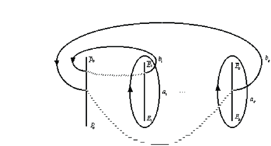
Figure 1: Homology basis of $\Sigma$

The theta functions are subject to a number of addition theorems. We will need the ternary addition theorem which can be cast in the form
Theorem 4.1: Ternary addition theorem
Let $[m_{i}]=[m_{i}^{1},m_{i}^{2}]$ $(i=1,\ldots,4)$ be arbitrary real $2g$-dimensional vectors. Then

$$\Theta[m_{1}](u+v)\Theta[m_{2}](u-v)\Theta[m_{3}](0)\Theta[m_{4}](0)$$ (30)

$$=\frac{1}{2^{g}}\sum\limits_{2a\in(Z_{2})^{2g}}\exp(-4\pi\mathrm{i}\langle m_{1}^{1},a^{2}\rangle)\Theta[n_{1}+a](u)\Theta[n_{2}+a](u)\Theta[n_{3}+a](v)\Theta[n_{4}+a](v),$$

where $a=(a^{1},a^{2})$, and $(m_{1},\dots,m_{4})=(n_{1},\dots,n_{4})T$ with

$$T=\frac{1}{2}\left(\begin{array}[]{rrrr}1&1&1&1\\ 1&-1&-1&-1\\ 1&-1&1&-1\\ 1&-1&-1&1\end{array}\right).$$ (31)

Each $1$ in $T$ denotes the $g\times g$ identity matrix.

For a proof see e.g. [26].

Let us recall that a divisor $X$ on $\Sigma$ is a formal symbol $X=n_{1}P_{1}+\ldots+n_{k}P_{k}$ with $P_{i}\in\Sigma$ and $n_{i}\in\mbox{Z}$. The degree of a divisor is $\sum_{i=1}^{k}n_{i}$. The Riemann vector $K_{R}$ is defined by the condition that $\Theta(\omega(W)+K_{R})=0$ if $W$ is a divisor of degree $g-1$ or less. We use here and in the following the notation $\omega(W)=\int_{P_{0}}^{W}\mathrm{d}\omega=\sum_{i=1}^{g-1}\omega(w_{i})$. We note that the Riemann vector can be expressed through half-periods in the case of a hyperelliptic surface.

The quotient of two theta functions with the same argument but different characteristic is a so-called root function which means that its square is a function on $\Sigma$. One can prove (see [26] and references therein)
Theorem 4.2: Root functions
Let $Q_{i}$, $i=1,\ldots,2g+2$, be the branch points of a hyperelliptic Riemann surface $\Sigma_{g}$ of genus $g$ and $A_{j}=\omega(Q_{j})$ with $\omega(Q_{1})=0$. Furthermore let $\{i_{1},\ldots,i_{g}\}$ and $\{j_{1},\ldots,j_{g}\}$ be two sets of numbers in $\{1,2,\ldots,2g+2\}$. Then the following equality holds for an arbitrary point $P\in\Sigma_{g}$,

$$\frac{\Theta\left[K_{R}+\sum_{k=1}^{g}A_{i_{k}}\right]\left(\omega(P)\right)}{\Theta\left[K_{R}+\sum_{k=1}^{g}A_{j_{k}}\right]\left(\omega(P)\right)}=c_{1}\sqrt{\frac{(K-E_{i_{1}})\ldots(K-E_{i_{g}})}{(K-E_{j_{1}})\ldots(K-E_{j_{g}})}},$$ (32)

where $c_{1}$ is a constant independent on $K$. Let $X=P_{1}+\ldots+P_{g}$ with $P_{j}=(K_{j},\mu(K_{j})$ be a divisor of degree g on $\Sigma_{g}$ then the following identity exists,

$$\frac{\Theta\left[K_{R}+A_{i}\right]\left(\omega(X)\right)}{\Theta\left[K_{R}+A_{j}\right]\left(\omega(X)\right)}=c_{2}\prod_{k=1}^{g}\sqrt{\frac{(K_{k}-Q_{i})}{(K_{k}-Q_{j})}},$$ (33)

where $c_{2}$ is a constant independent on the $K_{k}$.

The notion of divisors makes it possible to state Jacobi’s inversion theorem in a very compact form,
Theorem 4.3: Jacobi inversion theorem
Let $A,B\in\Sigma$ be divisors of degree g and $u\in\mathrm{C}^{g}$. Then for given $B$ and $u$, the equation $\omega(A)-\omega(B)=u$ for the divisor $A$ is always solvable.

For a proof we refer the reader to the standard literature, e.g. [25]. We remark that the divisor may not be uniquely defined in the general case which means that one or more $P_{i}\in A$ can be freely chosen. We will not consider such special cases in the following and refer the reader for the so-called special divisors to the literature as [26].

For divisors $A-B$ of degree zero, one can formulate Abel’s theorem.
Theorem 4.4: Abel’s theorem
Let $A,B\in\Sigma$ be divisors of degree $n$ subject to the relation $\omega(A)-\omega(B)=0$. Then $A$ and $B$ are the set of zeros respectively poles of a meromorphic function $F$.

For a proof see [25]. We remark that this function is a rational function on the surface cut along the homology basis. We have the

Corollary 4.5:
Let the condition of Abel’s theorem hold. Then the following identity holds for the integral of the third kind

$$\int_{B}^{A}d\omega_{PQ}=\ln\frac{F(P)}{F(Q)}.$$ (34)

4.2 Solutions to the Ernst equation

We are now able to write down a class of solutions to the Ernst equation on the surface $\Sigma$.
Theorem 4.5:
Let the Riemann surface $\Sigma$ be given by the relation $\mu^{2}(K)=(K+\mathrm{i}z)(K-\mathrm{i}z)\prod_{i=1}^{g}(K-E_{i})(K-\bar{E}_{i})$, let $u$ be the vector with the components $u_{i}=\frac{1}{2\pi\mathrm{i}}\int_{\Gamma}\ln Gd\omega_{i}$ where $\Gamma$ is as in theorem 2.1, let $G$ be subject to the condition $G(\tau)=\bar{G}(\bar{\tau})$, and let $[m]=[m^{1},m^{2}]$ with $m^{1}_{i}=0$ and $m^{2}_{i}$ arbitrary for $i=1,\ldots,g$ be a theta characteristic. Then the function $f$ given by

$$f(\rho,\zeta)=\frac{\Theta[m](\omega(\infty^{+})+u)}{\Theta[m](\omega(\infty^{-})+u)}\exp\left\{\frac{1}{2\pi\mathrm{i}}\int\limits_{\Gamma}\ln G(\tau)\mathrm{d}\omega_{\infty^{+}\infty^{-}}(\tau)\right\},$$ (35)

is a solution to the Ernst equation.
This class of solutions was first given by Korotkin [18], the straight forward continuous limit leading to the above form can be found in [27, 28]. For the relation to Riemann-Hilbert problems see [17]. In the case genus 0, the Ernst potential is real, and we get a solution of the Weyl class in the form (2). For higher genus, these solutions are in general non-static and thus generalize (2) to the stationary case.

In [29, 30] it was possible to identify a physically interesting subclass.

Theorem 4.6:
Let the conditions of Theorem 4.5 hold, and in addition let $\Sigma$ be a hyperelliptic Riemann surface of even genus $g=2n$ given by $\mu^{2}(K)=(K+\mathrm{i}z)(K-\mathrm{i}z)\prod_{i=1}^{n}(K^{2}-E_{i}^{2})(K^{2}-\bar{E}_{i}^{2})$, let the function $G$ be subject to the condition $G(-\tau)=G(\tau)$, and let $[n]$ be the characteristic with $n^{1}_{i}=0$ and $n^{2}_{i}=1$. Then the function $f$ given by

$$f(\rho,\zeta)=\frac{\Theta[n](\omega(\infty^{+})+u)}{\Theta[n](\omega(\infty^{-})+u)}\exp\left\{\frac{1}{2\pi\mathrm{i}}\int\limits_{\Gamma}\ln G(\tau)\mathrm{d}\omega_{\infty^{+}\infty^{-}}(\tau)\right\}$$ (36)

is an equatorially symmetric solution to the Ernst equation ($f(-\zeta)=\bar{f}(\zeta)$) which is everywhere regular except at the disk if $\Theta(\omega(\infty^{-})+u)\neq 0$.

For a proof see [29, 30] where one can also find how the characteristic can be generalized. In the following we will only use the characteristic of the above theorem.

A quantity of special interest is the metric function $a$. In [18] it was shown that one can relate it directly to theta functions without having to perform the integration of (11),

$$Z:=(a-a_{0})e^{2U}=D_{\infty^{-}}\ln\frac{\Theta(\omega(\infty^{-})+u)}{\Theta[n](\omega(\infty^{-})+u)}$$ (37)

where $D_{P}F(\omega(P))$ denotes the coefficient of the linear term in the expansion of the function $F(\omega(P))$ in the local parameter in the neighborhood of $P$, where $\Theta$ is the Riemann theta function with the characteristic $[m]$ and $m^{1}_{i}=m^{2}_{i}=0$, and where the constant $a_{0}$ is defined by the condition that $a$ vanishes on the regular part of the axis.

It is possible to give an algebraic representation of the solutions (36) (see [31] and [32]). We define the divisor $X=\sum_{i=1}^{g}K_{i}$ as the solution of the Jacobi inversion problem ($i=1,\ldots,g$)

$$\omega_{i}(X)-\omega_{i}(D)=\frac{1}{2\pi\mathrm{i}}\int_{\Gamma}\ln G\frac{\tau^{i-1}d\tau}{\mu(\tau)}=:\tilde{u}_{i},$$ (38)

where the divisor $D=\sum_{i=1}^{g}E_{i}$. With the help of these divisors, we can write (36) in the form

$$\ln f=\int_{D}^{X}\frac{\tau^{g}d\tau}{\mu(\tau)}-\frac{1}{2\pi\mathrm{i}}\int_{\Gamma}\ln G\frac{\tau^{g}d\tau}{\mu(\tau)},$$ (39)

Since the $\tilde{u}_{i}$ in (38) are just the periods of the second integral in (39), they are subject to a system of differential equations, the so-called Picard-Fuchs system (see [30] and references given therein). In our case this leads to

$$\sum_{n=1}^{g}\frac{(K_{n}-P_{0})K_{n}^{j}}{\mu(K_{n})}K_{n,z}=0,\quad j=0,...,g-2$$ (40)

and

$$(\ln f)_{z}=\sum_{n=1}^{g}\frac{(K_{n}-P_{0})K_{n}^{g-1}}{\mu(K_{n})}K_{n,z}.$$ (41)

Solving for the $K_{n,z}$, $n=1,\ldots,g$, we get

$$K_{n,z}=(\ln f)_{z}\frac{\mu(K_{n})}{K_{n}-P_{0}}\frac{1}{\prod_{m=1,m\neq n}^{g}(K_{n}-K_{m})}.$$ (42)

Additional information follows from the reality of the $\tilde{u}_{i}$ which implies $\omega(X)-\omega(D)=\omega(\bar{X})-\omega(\bar{D})$. Using Abel’s theorem on this condition, we obtain the relation for an arbitrary $K\in\mbox{C}$

$$(1-x^{2})\prod_{i=1}^{g}(K-K_{i})(K-\bar{K}_{i})=\prod_{i=1}^{g}(K-E_{i})(K-\bar{E}_{i})-(K-P_{0})(K-\bar{P}_{0})Q_{2}^{2}(K),$$ (43)

where with purely imaginary $x_{i}$, $x$

$$Q_{2}(K)=x_{0}+x_{1}K+...+x_{g-2}K^{g-2}+xK^{g-1}.$$ (44)

Since (43) has to hold for all $K\in\mbox{C}$, it is equivalent to $2g$ real algebraic equations for the $K_{i}$ if the $x_{i}$ are given. Using (34) and (39) we find

$$\frac{f}{\bar{f}}=\frac{1+x}{1-x}$$ (45)

which implies $x=\mathrm{i}be^{-2U}$.

Remark: To solve boundary value problems with the class of solutions (36), one has two kinds of freedom: the function $G$ as before and the branch points $E_{i}$ of the Riemann surface as a discrete degree of freedom. Since one would need to specify two free functions to solve a general boundary value problem for the Ernst equation, it is obvious that one can only solve a restricted class of problems on a given surface, and that one cannot expect to solve general problems on a surface of finite genus. But once one has constructed a solution which takes the imposed boundary data at the disk, one has to check the condition $\Theta(\omega(\infty^{-})+u)\neq 0$ in the whole spacetime to actually prove that one has found the desired solution: a solution that is everywhere regular except at the disk where it has to take the imposed boundary conditions.

There are in principle two ways of generalizing the approach used for the Newtonian case: One can eliminate $\Omega$ from the two real equations (23) and enter the resulting equation with a solution (36) on a chosen Riemann surface. This will lead for given $\gamma$ to a non-linear integral equation for $\ln G$. In general there is little hope to get explicit solutions to this equation (for a numerical treatment of differentially rotating disks along this line in the genus 2 case see [33]). Once a function $G$ is found, one can read off the rotation law $\Omega$ on a given Riemann surface from (36). Another approach is to establish the relations between the real and the imaginary part of the Ernst potential which exist on a given Riemann surface for arbitrary $G$. The simplest example for such a relation is provided by the function $w=e^{\mathrm{i}\psi}$ which is a function on a Riemann surface of genus 0, where we have obviously $|w|=1$. As we will point out in the following, similar relations also exist for an Ernst potential of the form (36), but they will lead to a system of differential equations. Once one has established these relations for a given Riemann surface, one can determine in principle which boundary value problems can be solved there (in our example which classes of functions $\Omega$, $\gamma$ can occur) by the condition that one of the boundary conditions must be identically satisfied. The second equation will then be used to determine $G$ as the solution of an integral equation which is possibly non-linear. Following the second approach, we want to study the implications of the hyperelliptic Riemann surface for the physical properties of the solutions.

5 Axis Relations

In order to establish relations between the real and the imaginary part of the Ernst potential, we will first consider the axis of symmetry ($\rho=0$) where the situation simplifies decisively. In addition the axis is of interest since the asymptotically defined multipole moments [34, 35] can be read off there [36].

On the axis the Ernst potential can be expressed through functions defined on the Riemann surface $\Sigma^{\prime}$ given by $\mu^{\prime}{}^{2}=\prod_{i=1}^{g}(K-E_{i})(K-\bar{E}_{i})$, i.e. the Riemann surface obtained from $\Sigma$ by removing the cut $[P_{0},\bar{P}_{0}]$ which just collapses on the axis. We use the notation of the previous section and let a prime denote that the corresponding quantity is defined on the surface $\Sigma^{\prime}$. The cut system is as in the previous section with $[E_{1},\bar{E}_{1}]$ taking the role of $[P_{0},\bar{P}_{0}]$ (all $b$-cuts cross $[E_{1},\bar{E}_{1}]$). We choose the Abel map in a way that $\omega^{\prime}(E_{1})=0$. It was shown in [30] that for genus $g>1$ the Ernst potential takes the form (for $\zeta>0$)

$$f(0,\zeta)=\frac{\vartheta\left(\int_{\zeta^{+}}^{\infty^{+}}\mathrm{d}\omega^{\prime}+u^{\prime}\right)-\exp(-(\omega^{\prime}_{g}(\infty^{+})+u_{g}))\vartheta\left(\int_{\zeta^{-}}^{\infty^{+}}\mathrm{d}\omega^{\prime}+u^{\prime}\right)}{\vartheta\left(\int_{\zeta^{+}}^{\infty^{+}}\mathrm{d}\omega^{\prime}-u^{\prime}\right)-\exp(-(\omega^{\prime}_{g}(\infty^{+})-u_{g}))\vartheta\left(\int_{\zeta^{-}}^{\infty^{+}}\mathrm{d}\omega^{\prime}-u^{\prime}\right)}e^{I+u_{g}},$$ (46)

where $\vartheta$ is the theta function on $\Sigma^{\prime}$ with the characteristic $\alpha_{i}^{\prime}=0$, $\beta_{i}^{\prime}=1$ for $i=1,\ldots,g-1$, where $I=\frac{1}{2\pi\mathrm{i}}\int\limits_{\Gamma}\ln G(\tau)\mathrm{d}\omega^{\prime}_{\infty^{+}\infty^{-}}(\tau)$, $\mathrm{d}\omega_{g}=\mathrm{d}\omega_{\zeta^{-}\zeta^{+}}$, and where $u_{g}=\frac{1}{2\pi\mathrm{i}}\int\limits_{\Gamma}\ln G(\tau)\mathrm{d}\omega_{g}(\tau)$.

Notice that the $u_{i}^{\prime}$ and $I$ are constant with respect to $\zeta$. The only term dependent both on $G$ and on $\zeta$ is $u_{g}$. To establish a relation on the axis between the real and the imaginary part of the Ernst potential independent of $G$, the first step must be thus to eliminate $u_{g}$. We can state the following

Theorem 4.1:
The Ernst potential (46) satisfies for $g>1$ the relation

$$P_{1}(\zeta)f\bar{f}+P_{2}(\zeta)b+P_{3}(\zeta)=0,$$ (47)

where the $P_{i}$ are real polynomials in $\zeta$ with coefficients depending on the branch points $E_{i}$ and the $g$ real constants $\int_{\Gamma}\ln G\tau^{i}d\tau/\mu^{\prime}(\tau)$ with $i=0,\ldots,g-1$. The degree of the polynomials $P_{1}$ and $P_{3}$ is $2g-3$ or less, the degree of $P_{2}$ is $2g-2$ or less.

To prove this theorem we need the fact that one can express integrals of the third kind via theta functions with odd characteristic denoted by $\vartheta_{o}$,

$$\exp(-\omega_{g}(\infty^{+}))=-\frac{\vartheta_{o}(\omega^{\prime}(\infty^{+})-\omega^{\prime}(\zeta^{+}))}{\vartheta_{o}(\omega^{\prime}(\infty^{+})-\omega^{\prime}(\zeta^{-}))}.$$ (48)

Proof:
The first step is to establish the relation

$$Af\bar{f}+B\mathrm{i}b+1=0,$$ (49)

where

$$Ae^{2I}=-\frac{\vartheta\left(u^{\prime}+\int_{\zeta^{-}}^{\infty^{-}}\mathrm{d}\omega^{\prime}\right)\vartheta\left(u^{\prime}+\int_{\zeta^{+}}^{\infty^{-}}\mathrm{d}\omega^{\prime}\right)}{\vartheta\left(u^{\prime}+\int_{\zeta^{-}}^{\infty^{+}}\mathrm{d}\omega^{\prime}\right)\vartheta\left(u^{\prime}+\int_{\zeta^{+}}^{\infty^{+}}\mathrm{d}\omega^{\prime}\right)}$$ (50)

and

$$Be^{I}=\frac{e^{-\omega_{g}(\infty^{+})}\vartheta\left(u^{\prime}+\int_{\zeta^{-}}^{\infty^{+}}\mathrm{d}\omega^{\prime}\right)\vartheta\left(u^{\prime}+\int_{\zeta^{+}}^{\infty^{-}}\mathrm{d}\omega^{\prime}\right)+e^{\omega_{g}(\infty^{+})}\vartheta\left(u^{\prime}+\int_{\zeta^{+}}^{\infty^{+}}\mathrm{d}\omega^{\prime}\right)\vartheta\left(u^{\prime}+\int_{\zeta^{-}}^{\infty^{-}}\mathrm{d}\omega^{\prime}\right)}{\vartheta\left(u^{\prime}+\int_{\zeta^{-}}^{\infty^{+}}\mathrm{d}\omega^{\prime}\right)\vartheta\left(u^{\prime}+\int_{\zeta^{+}}^{\infty^{+}}\mathrm{d}\omega^{\prime}\right)}$$ (51)

which may be checked with (46) by direct calculation. The reality properties of the Riemann surface $\Sigma^{\prime}$ and the function $G$ imply that $A$ is real and that $B$ is purely imaginary. We use the addition theorem (30) with $[m_{1}]=\ldots=[m_{4}]$ equal to the characteristic of $\vartheta$ for (50) to get

$$Ae^{2I}=-\frac{\sum\limits_{2a\in(Z_{2})^{2g}}\exp(-4\pi\mathrm{i}\langle m_{1}^{1},a^{2}\rangle)\vartheta^{2}[a](u^{\prime}+\omega^{\prime}(\infty^{-}))\vartheta^{2}[a](\omega^{\prime}(\zeta^{+}))}{\sum\limits_{2a\in(Z_{2})^{2g}}\exp(-4\pi\mathrm{i}\langle m_{1}^{1},a^{2}\rangle)\vartheta^{2}[a](u^{\prime}+\omega^{\prime}(\infty^{+}))\vartheta^{2}[a](\omega^{\prime}(\zeta^{+}))}.$$ (52)

This term is already in the desired form. Using the relation for root functions (32), one can directly see that the right-hand side is a quotient of polynomials of order $g-1$ or lower in $\zeta$. For (51) we use (48) with $[\tilde{m}_{1}]=[\tilde{m}_{2}]=[K_{R}]$ as the characteristic of the odd theta function $\vartheta_{o}$ and let $[\tilde{m}_{3}]=[\tilde{m}_{4}]$ be equal to the characteristic of $\vartheta$. The addition theorem (30) then leads to

$$Be^{I} = -\frac{\sum\limits_{2a\in(Z_{2})^{2g}}\exp(-4\pi\mathrm{i}\langle\tilde{m}_{1}^{1},a^{2}\rangle)\Theta^{\prime 2}[n+a](u^{\prime}+\omega^{\prime}(\infty^{-}))\vartheta^{2}[a](\omega^{\prime}(\zeta^{+}))}{\sum\limits_{2a\in(Z_{2})^{2g}}\exp(-4\pi\mathrm{i}\langle m_{1}^{1},a^{2}\rangle)\vartheta^{2}[a](u^{\prime}+\omega^{\prime}(\infty^{+}))\vartheta^{2}[a](\omega^{\prime}(\zeta^{+}))}\times$$ (53)

$$\sum\limits_{2a\in(Z_{2})^{2g}}\exp(-4\pi\mathrm{i}\langle m_{1}^{1},a^{2}\rangle)\frac{\vartheta^{2}[a](u^{\prime})}{\vartheta^{2}(0)}\times$$

$$\left(\frac{\vartheta^{2}[a](\omega^{\prime}(\infty^{+})-\omega^{\prime}(\zeta^{+}))}{\vartheta_{o}^{2}(\omega^{\prime}(\infty^{+})-\omega^{\prime}(\zeta^{+}))}+\frac{\vartheta^{2}[a](\omega^{\prime}(\infty^{+})-\omega^{\prime}(\zeta^{-}))}{\vartheta_{o}^{2}(\omega^{\prime}(\infty^{+})-\omega^{\prime}(\zeta^{-}))}\right),$$

where $n$ follows from $\tilde{m}$ as in Theorem 4.1. The first fraction in (53) is again the quotient of polynomials of degree $g-1$ in $\zeta$ for the same reasons as above. But since the quotient must vanish for $\zeta\to\infty$, the leading terms in the numerator just cancel. It is thus a quotient of polynomials of degree $g-2$ or less in the numerator and $g-1$ or less in the denominator. To deal with the quotients $\vartheta^{2}[a](\omega^{\prime}(\infty^{+})-\omega^{\prime}(\zeta^{\pm}))/\vartheta_{o}^{2}(\omega^{\prime}(\infty^{+})-\omega^{\prime}(\zeta^{\pm}))$, we define the divisors $T^{\pm}=T_{1}^{\pm}+\ldots+T_{g-1}^{\pm}$ as the solutions of the Jacobi inversion problems $\omega^{\prime}(T^{\pm})-\omega^{\prime}(Y)=\omega^{\prime}(\infty^{+})+\omega^{\prime}(\zeta^{\pm})$ where $Y$ is the divisor $Y=E_{1}+\ldots+E_{g-1}$. Abel’s theorem then implies for arbitrary $K\in\mbox{C}$

$$\prod_{i=1}^{g-1}(K-T_{i}^{\pm})(K-\zeta)=(K-A^{\pm})^{2}\prod_{i=1}^{g-1}(K-E_{i})-(K-E_{g})\prod_{i=1}^{g}(K-\bar{E}_{i}),$$ (54)

where

$$\zeta-A^{\pm}=\pm\frac{\mu^{\prime}(\zeta)}{\prod_{i=1}^{g-1}(\zeta-E_{i})}.$$ (55)

Let $Q_{j}$ be given by the condition $[Q_{j}+K_{R}]=[a]$, i.e. $Q_{j}$ is a branch point of $\Sigma^{\prime}$. Then we get for the quotient

$$\frac{\vartheta^{2}[a](\omega^{\prime}(\infty^{+})-\omega^{\prime}(\zeta^{\pm}))}{\vartheta_{o}^{2}(\omega^{\prime}(\infty^{+})-\omega^{\prime}(\zeta^{\pm}))}=const\prod_{i=1}^{g-1}\frac{T^{\pm}_{i}-Q_{j}}{T^{\pm}_{i}-E_{1}},$$ (56)

where $const$ is a $\zeta$-independent constant. With the help of (54), it is straight forward to see that for $Q_{j}\in Y$, the theta quotient is just proportional to $(\zeta-E_{1})/(\zeta-Q_{j})$ whereas for $Q_{j}\notin Y$, the term is proportional to $(\zeta-E_{1})(Q_{j}-A^{\pm})^{2}/(\zeta-Q_{j})$. Using (55) one recognizes that the terms containing roots just cancel in (53). The remaining terms are just quotients of polynomials in $\zeta$ with maximal degree $g$ in the numerator and $g-2$ in denominator. This completes the proof.

Remark: The remaining dependence on $G$ through $u^{\prime}$ and $I$ can only be eliminated by differentiating relation (46) $g$ times. If we prescribe e.g. the function $b$ on a given Riemann surface (this just reflects the fact that the function $G$ can be freely chosen in (46)), we can read off $e^{2U}$ from (47). To fix the constants related to $G$ in (47) one needs to know the Ernst potential and $g-1$ derivatives at some point on the axis where the Ernst potential is regular, e.g. at the origin or at infinity, where one has to prescribe the multipole moments. If the Ernst potential were known on some regular part of the axis, one could use (47) to read off the Riemann surface (genus and branch points). Equation (46) is then an integral equation for $G$ for known sources. This just reflects a result of [37] that the Ernst potential for known sources can be constructed via Riemann-Hilbert techniques if it is known on some regular part of the axis.

In practice it is difficult to express the coefficients in the polynomials $P_{i}$ via the constants $u_{i}^{\prime}$ and $I$, and it will be difficult to get explicit expressions. We will therefore concentrate on the general structure of the relation (47), its implications on the multipoles and some instructive examples. Let us first consider the case genus 1 which is not generically equatorially symmetric. In this case the Riemann surface $\Sigma^{\prime}$ is of genus 0. One can use formula (46) for the axis potential if one replaces the theta functions by 1. We thus end up with

$$f\bar{f}-2b\frac{\zeta-\alpha_{1}}{\beta_{1}}e^{I}=e^{2I}.$$ (57)

Here the only remaining $G$-dependence is in $I$. If $f_{0}=f(0,0)$ is given, $e^{I}$ follows from $f_{0}\bar{f}_{0}+2b_{0}\alpha_{1}e^{I}/\beta_{1}=e^{2I}$, if the in general non-real mass $M$ is known, the constant $e^{I}$ follows from $1+4\mbox{Im}Me^{I}/\beta_{1}=e^{2I}$. In the latter case the imaginary part of the Arnowitt-Deser-Misner mass (this corresponds to a NUT-parameter) will be sufficient. Differentiating (57) once will lead to a differential relation between the real and the imaginary part of the Ernst potential which holds for all $G$, which means it reflects only the impact of the underlying Riemann surface on the structure of the solution.

Remark: For equatorially symmetric solutions, one has on the positive axis the relation $f(-\zeta)\bar{f}(\zeta)=1$ (see [38, 39], this is to be understood in the following way: the function $|\zeta|$ is even in $\zeta$, but restricted to positive $\zeta$ it seems to be an odd function, and it is exactly this behavior which is addressed by the above formula). This leads to the conditions

$$P_{1}(-\zeta)=-P_{3}(\zeta),\quad P_{2}(-\zeta)=P_{2}(\zeta).$$ (58)

The coefficients in the polynomials depend on the $g/2$ integrals $\int_{\Gamma}d\tau\ln G\tau^{2i}/\mu^{\prime}(\tau)$ ($i=0,\ldots,g/2-1$ and the branch points.

The simplest interesting example is genus 2, where we get with $E_{1}^{2}=\alpha+\mathrm{i}\beta$

$$f\bar{f}(\zeta-C_{1})+\frac{\sqrt{2}}{C_{2}}(\zeta^{2}-\alpha-C_{2}^{2})b=\zeta+C_{1},$$ (59)

i.e. a relation which contains two real constants $C_{1}$, $C_{2}$ related to $G$. In case that the Ernst potential at the origin is known, one can express these constants via $f_{0}$. A relation of this type, which is as shown typical for the whole class of solutions, was observed in the first paper of [21] for the rigidly rotating dust disk.

6 Differential relations in the whole spacetime

The considerations on the axis have shown that it is possible there to obtain relations between the real and the imaginary part of the Ernst potential which are independent of the function $G$ and thus reflect only properties of the underlying Riemann surface. The found algebraic relations contain however $g$ real constants related to the function $G$, which means that one has to differentiate $g$ times to get a differential relation which is completely free of the function $G$. These constants were just the integrals $u^{\prime}$ and $I$ which are only constant with respect to the physical coordinates on the axis where the Riemann surface $\Sigma$ degenerates. Thus one cannot hope to get an algebraic relation in the whole spacetime as on the axis. Instead one has to deal with integral equations or to look directly for a differential relation.

To avoid the differentiation of theta functions with respect to a branch point of the Riemann surface, we use the algebraic formulation of the hyperelliptic solutions (38) and (39). From the latter it can also be seen how one could get a relation independent of $G$ without differentiation: one can consider the equations (38) and (39) as integral equations for $G$. In principle one could try to eliminate $G$ and $X$ from these equations and (43). We will not investigate this approach but try to establish a differential relation. To this end it proves helpful to define the symmetric (in the $K_{n}$) functions $S_{i}$ via

$$\prod_{i=1}^{g}(K-K_{i})=:K^{g}-S_{g-1}K^{g-1}+...+S_{0}$$ (60)

i.e. $S_{0}=K_{1}K_{2}\ldots K_{g}$, …, $S_{g-1}=K_{1}+\ldots+K_{g}$. The equations (43) are bilinear in the real and imaginary parts of the $S_{i}$ which are denoted by $R_{i}$ and $I_{i}$ respectively. With this notation we get

Theorem 6.1:
The $x_{i}$ and the Ernst potential $f$ are subject to the system of differential equations

$$0 = \left(R_{0}-P_{0}R_{1}+\ldots+P_{0}^{g}(-1)^{g}\right)x_{z}-\frac{\mathrm{i}}{2}Q_{2}(P_{0})$$ (61)

$$-\frac{\mathrm{i}}{2}(1-x^{2})(\ln f\bar{f})_{z}\left(I_{0}-P_{0}I_{1}+\ldots+(-1)^{g-1}I_{g-1}P_{0}^{g-1}\right)$$

and for $g>1$

$$x_{j,z} = x_{z}\left((-1)^{j+1}R_{j+1}+\ldots+P_{0}^{g-j-1}\right)-\mathrm{i}(x_{j+1}+\ldots+xP_{0}^{g-j-2})$$ (62)

$$-\frac{\mathrm{i}}{2}(1-x^{2})(\ln f\bar{f})_{z}(((-1)^{j+1}I_{j+1}+\ldots-P_{0}^{g-j-2}I_{g-1}).$$

Proof:
Differentiating (43) with respect to $z$ and eliminating the derivatives of the $K_{i,z}$ via the Picard-Fuchs relations (42), we end up with a linear system of equations for the derivatives of the $x_{i}$ and $x$ which can be solved in standard manner. The Vandemonde-type determinants can be expressed via the symmetric functions. For $x_{z}$ one gets (61). The equations for the $x_{j,z}$ are bilinear in the symmetric functions. They can be combined with (61) to (62).

Remark: If one can solve (43) for the $K_{i}$, the equations (61) and (62) will be a non-linear differential system in $z$ (and $\bar{z}$ which follows from the reality properties) for the $x_{i}$, $x$ and $f$ which only contains the branch points of the Riemann surface as parameters.

For the metric function $a$, we get with (37)

Theorem 6.2:
The metric function $a$ is related to the functions $x_{i}$ and $S_{i}$ via

$$Z=\frac{\mathrm{i}x_{g-2}}{1-x^{2}}-I_{g-1}-\frac{\mathrm{i}x\zeta}{1-x^{2}}.$$ (63)

for $g>1$ and

$$Z=-I_{0}+\frac{\mathrm{i}x(\alpha_{1}-\zeta)}{1-x^{2}}$$ (64)

for $g=1$.

Proof:
To express the function $Z$ via the divisor $X$, we define the divisor $T=T_{1}+\ldots+T_{g}$ as the solution of the Jacobi inversion problem $\omega(T)=\omega(X)+\omega(P)$ where $P$ is in the vicinity of $\infty^{-}$ (only terms of first order in the local parameter near $\infty^{-}$ are needed). Using the formula for root functions (33), we get for the quantity $Z$ in (37)

$$Z=\frac{\mathrm{i}}{2}D_{\infty^{-}}\ln\prod_{i=1}^{g}\frac{T_{i}-\bar{P}_{0}}{T_{i}-P_{0}}.$$ (65)

Applying Abel’s theorem to the definition of $T$ and expanding in the local parameter near $\infty^{-}$, we end up with (63) for general $g>1$ and with (64) for $g=1$.

Remark:
1. For $g>1$ equation (63) can be used to replace the relation for $x_{g-2,z}$ in (62) since the latter is identically fulfilled with (63) and (11).

2. An interesting limiting case is $G\approx 1$ where $f\approx 1$, i.e. the limit where the solution is close to Minkowski spacetime. By the definition (38), the divisor $X$ is in this case approximately equal to $D$. Thus the symmetric functions in (62) and (61) can be considered as being constant and given by the branch points $E_{i}$. Relation (63) implies that the quantity $Z$ is approximately equal to $I_{g-2}$ in this limit, i.e. it is mainly equal to the constant $a_{0}$ in lowest order. Since the differential system (62) and (61) is linear in this limit, it is straight forward to establish two real differential equations of order $g$ for the real and the imaginary part of the Ernst potential. In principle this works also in the non-linear case, where sign ambiguities in the solution of (38) can be fixed by the Minkowskian limit.

To illustrate the above equations we will first consider the elliptic case. This is the only case where one can establish an algebraic relation between $Z$ and $b$ independent of $G$. Equations (43) lead to

$$(1-x^{2})R_{0} = \alpha_{1}-\zeta x^{2}$$

$$(1-x^{2})S_{0}\bar{S}_{0} = E_{1}\bar{E}_{1}-P_{0}\bar{P}_{0}x^{2}.$$ (66)

Formula (64) takes with (66) (the sign of $I_{0}$ is fixed by the condition that $I_{0}=-\beta_{1}$ for $x=0$) the form

$$(1-x^{2})Z=\mathrm{i}x(\alpha_{1}-\zeta)+\sqrt{(1-x^{2})(\beta_{1}^{2}-\rho^{2}x^{2})-x^{2}(\alpha_{1}-\zeta)^{2}}.$$ (67)

This relation holds in the whole spacetime for all elliptic potentials, i.e. for all possible choices of $G$ in (36). This implies that one can only solve boundary value problems on elliptic surfaces where the boundary data at some given contour $\Gamma_{z}$ satisfy condition (67).

In the case genus 2, we get for (43)

$$(1-x^{2})R_{1} = \alpha_{1}+\alpha_{2}-\zeta x^{2}+xx_{0},$$

$$(1-x^{2})(R_{1}^{2}+I_{1}^{2}+2R_{0}) = (\alpha_{1}+\alpha_{2})^{2}+2\alpha_{1}\alpha_{2}+\beta_{1}^{2}+\beta_{2}^{2}-x_{0}^{2}-x^{2}(\rho^{2}+\zeta^{2})+4\zeta xx_{0},$$

$$(1-x^{2})(R_{1}R_{0}+I_{1}I_{0}) = \alpha_{1}\alpha_{2}(\alpha_{1}+\alpha_{2})+\alpha_{1}\beta_{2}^{2}+\alpha_{2}\beta_{1}^{2}-\zeta x_{0}^{2}+(\rho^{2}+\zeta^{2})xx_{0},$$

$$(1-x^{2})(R_{0}^{2}+I_{0}^{2}) = (\alpha_{1}^{2}+\beta_{1}^{2})(\alpha_{2}^{2}+\beta_{2}^{2})-(\rho^{2}+\zeta^{2})x_{0}^{2}.$$ (68)

The aim is to determine the $S_{i}$ and $x_{0}$ from (68) and

$$(1-x^{2})(Z+I_{1})=\mathrm{i}x_{0}-\zeta\mathrm{i}x,$$ (69)

and to eliminate these quantities in

$$(R_{0}-P_{0}R_{1}+P_{0}^{2})x_{z}=\frac{\mathrm{i}}{2}(x_{0}+P_{0}x)+\frac{\mathrm{i}}{2}(1-x^{2})(\ln f\bar{f})_{z}(I_{0}-P_{0}I_{1})$$ (70)

which follows from (61).

Remark: Boundary value problems
Since the above relations will hold in the whole spacetime, it is possible to extend them to an arbitrary smooth boundary $\Gamma_{z}$, where the Ernst potential may be singular (a jump discontinuity) and where one wants to prescribe boundary data (combinations of $f$, $f_{z}$). If these data are of sufficient differentiability (at least $C^{g,\alpha}(\Gamma_{z})$), we can check the solvability of the problem on a given surface with the above formulas. The conditions on the differentiability of the boundary data can be relaxed by working directly with the equations (38) and (39) which can be considered as integral equations for $\ln G$. The latter is not very convenient if one wants to construct explicit solutions, but it makes it possible to treat boundary value problems where the boundary data are Hölder continuous. We will only work with the differential relations and consider merely the derivatives tangential to $\Gamma_{z}$ in (62) to establish the desired differential relations between $a$, $b$ and $U$. One ends up with two differential equations which involve only $U$, $b$ and derivatives. The aim is to construct the spacetime which corresponds to the prescribed boundary data from these relations. To this end one has to integrate the differential relations using the boundary conditions. Integrating one of these equations, one gets $g$ real integration constants which cannot be freely chosen since they arise from applying the tangential derivatives in (62). Thus they have to be fixed in a way that the integrals on the right-hand side of (38) are in fact the $b$-periods of the second integral on the right-hand side of (38) and that (39) holds. The second differential equation arises from the use of normal derivatives of the Ernst potential in (61). To satisfy the $b$-period condition (38), one has to fix a free function in the integrated form of the corresponding differential equation. Thus one has to complement the two differential equations following from (61) with an integral equation which is obtained by eliminating $G$ from e.g. $\tilde{u}_{1}$ and $\tilde{u}_{2}$ in (38). For given boundary data, the system following from (38) may in principle be integrated to give $e^{2U}$ and $b$ in dependence of the boundary data. Then the in general non-linear integral equation will establish whether the boundary data are compatible with the considered Riemann surface. This is typically a rather tedious procedure. There is however a class of problems where it is unnecessary to use this integral equation. In case that the differential equations hold for an arbitrary function $e^{2U}$, the integral equation will only be used to determine this metric function, but the boundary value problem will be always solvable (locally). This offers a constructive approach to solve boundary value problems without having to consider non-linear integral equations.

7 Counter-rotating disks of genus 2

Since it is not very instructive to establish the differential relations for genus 2 in the general case, we will concentrate in this section on the form these equations take in the equatorially symmetric case for counter-rotating dust disks. In this case, the solutions are parametrized by $E_{1}^{2}=\alpha+\mathrm{i}\beta$. We will always assume in the following that the boundary data are at least $C^{2}(\Gamma_{z})$ (the normal derivatives of the metric functions have a jump at the disk, but the tangential derivatives are supposed to exist up to at least second order). Putting $s=be^{-2U}$ and $y=e^{2U}$, we get for (70) for $\zeta=0$, $\rho\leq 1$

$$\mathrm{i}x_{0} = \left(R_{0}-\rho^{2}-sI_{0}\right)\frac{b_{\zeta}}{y}-\rho\left(R_{1}-sI_{1}\right)\frac{b_{\rho}}{y}-\left(s(R_{0}-\rho^{2})+I_{0}\right)\frac{y_{\zeta}}{y}+\rho\left(sR_{1}+I_{1}\right)\frac{y_{\rho}}{y},$$

$$\rho s = \left(R_{0}-\rho^{2}-sI_{0}\right)\frac{b_{\rho}}{y}+\rho\left(R_{1}-sI_{1}\right)\frac{b_{\zeta}}{y}-\left(s(R_{0}-\rho^{2})+I_{0}\right)\frac{y_{\rho}}{y}-\rho\left(sR_{1}+I_{1}\right)\frac{y_{\zeta}}{y},\quad\quad$$ (71)

where the $S_{i}$ and $\mathrm{i}x_{0}$ are taken from (68) and (69). Since counter-rotating dust disks are subject to the boundary conditions (23), we can replace the normal derivatives in (71) via (23) which leads to a differential system where only tangential derivatives at the disk occur. With (68) and (69) we get

$$\mathrm{i}x_{0}+(Z-\mathrm{i}x_{0})\frac{R_{0}-\rho^{2}}{I_{1}R} = \left(\rho-\frac{R^{2}+\rho^{2}+\delta y^{2}}{2R\rho}\frac{R_{0}-\rho^{2}}{I_{1}}\right)\left((-Z+\mathrm{i}x_{0})\frac{y_{\rho}}{y}-sZ\frac{b_{\rho}}{y}\right),$$ (72)

$$\rho s\left(1-\frac{Z}{R}\right) = \left(\frac{R_{0}-\rho^{2}}{I_{1}}-\frac{R^{2}+\rho^{2}+\delta y^{2}}{2R}\right)\left(sZ\frac{y_{\rho}}{y}+(-Z+\mathrm{i}x_{0})\frac{b_{\rho}}{y}\right).\quad\quad$$ (73)

With $I_{1}=\mathrm{i}x_{0}/(1-x^{2})-Z$ and

$$R_{0}=\frac{\mathrm{i}x_{0}Z-\alpha-\frac{\rho^{2}}{2}}{1-x^{2}}-\frac{Z^{2}-\rho^{2}}{2},$$ (74)

the function $\mathrm{i}x_{0}$ follows from

$$R_{0}^{2}+\frac{(R_{0}-\rho^{2})^{2}}{I_{1}^{2}}\frac{x^{2}x_{0}^{2}}{(1-x^{2})^{2}}=\frac{\alpha^{2}+\beta^{2}-\rho^{2}x_{0}^{2}}{1-x^{2}},$$ (75)

i.e. an algebraic equation of fourth order for $\mathrm{i}x_{0}$ which can be uniquely solved by respecting the Minkowskian limit. Thus (72) and (73) are in fact a differential system which determines $b$ and $y$ in dependence of the angular velocity $\Omega$.

7.1 Newtonian limit

For illustration we will first study the Newtonian limit of the equations (73) (where counter-rotation does not play a role). This means we are looking for dust disks with an angular velocity of the form $\Omega=\omega q(\rho)$ where $|q(\rho)|\leq 1$ for $\rho\leq 1$, and where the dimensionless constant $\omega<<1$. Since we have put the radius $\rho_{0}$ of the disk equal to 1, $\omega=\omega\rho_{0}$ is the upper limit for the velocity in the disk. The condition $\omega<<1$ just means that the maximal velocity in the disk is much smaller than the velocity of light which is equal to 1 in the used units. An expansion in $\omega$ is thus equivalent to a standard post-Newtonian expansion. Of course there may be dust disks of genus 2 which do not have such a limit, but we will study in the following which constraints are imposed by the Riemann surface on the Newtonian limit of the disks where such a limit exists.

The invariance of the metric (10) under the transformation $t\to-t$ and $\Omega\to-\Omega$ implies that $U$ is an even function in $\omega$ whereas $b$ has to be odd. Since we have chosen an asymptotically non-rotating frame, we can make the ansatz $y=1+\omega^{2}y_{2}+\ldots$, $b=\omega^{3}b_{3}+\ldots$, and $a=\omega^{3}a_{3}+\ldots$. The boundary conditions (23) imply in lowest order $y_{2,\rho}=2q^{2}\rho$, the well-known Newtonian limit. Since (12) reduces to the Laplace equation for $y_{2}$ in order $\omega^{2}$, we can use the methods of section (2) to construct the corresponding solution. In order $\omega^{3}$, the boundary conditions (23) lead to

$$b_{3,\rho}=2\rho qy_{2,\zeta},$$ (76)

whereas equation (12) leads to the Laplace equation for $b_{3}$. Again we can use the methods of section 2, but this time we have to construct a solution which is odd in $\zeta$ because of the equatorial symmetry. In principle one can extend this perturbative approach to higher order, where the field equations (12) lead to Poisson equations with terms of lower order acting as source terms, and where the boundary conditions can also be obtained iteratively from (23).

With this notation we get
Theorem 7.1:
Dust disks of genus 2 which have a Newtonian limit, i.e. a limit in which $\Omega=\omega q(\rho)$ where $|q(\rho)|\leq 1$ for $\rho\leq 1$, are either rigidly rotating ($q=1$) or $q$ is a solution to the integro-differential equation

$$b_{3}=\left((R_{0}^{0}-\rho^{2})2q-\kappa\right)y_{2,\zeta}$$ (77)

where in the first case $I_{1}^{0}/R_{0}^{0}=2\omega$ and in the second $I_{1}=\kappa\omega$ with $R_{0}^{0}$ and $\kappa$ being $\omega$ independent constants.

Proof:
Since the right hand side of (38) vanishes, we have $K_{i}=E_{i}$ for $\omega\to 0$, and thus $a_{0}=I_{1}$ up to at least order $\omega^{3}$. Keeping only terms in lowest order and denoting the corresponding terms of the symmetric functions by $S_{i}^{0}$, we obtain for (73)

$$\omega^{3}b_{3}=y_{2,\zeta}\left(2q(R^{0}_{0}-\rho^{2})\omega^{3}-\omega^{2}I^{0}_{1}\right).$$ (78)

The second equation (73) involves $b_{3,\zeta}$ and is thus of higher order. If (78) holds, this equation will be automatically fulfilled.

The $\omega$-dependence in (78) implies that $R_{0}^{0}$, $I_{1}^{0}$ and thus the branch points must depend on $\omega$. Since $y_{2,\zeta}$ is proportional to the density in the Newtonian case, it must not vanish identically. The possible cases following from equation (78) are constant $\Omega$ or (77). Using (6) and (3), one can express $U_{\zeta}$ directly via $\Omega$ which leads to

$$y_{2,\zeta}=\frac{4}{\pi}\int_{0}^{1}\frac{\mathrm{d}\rho^{\prime}}{\rho+\rho^{\prime}}\partial_{\rho^{\prime}}(q^{2}\rho^{\prime}{}^{2})K(k)$$ (79)

with $k=2\sqrt{\rho\rho^{\prime}}/(\rho+\rho^{\prime})$. Thus (77) is in fact an integro-differential equation for $q$. This completes the proof.

7.2 Explicit solution for constant angular velocity and constant relative density

The simplifications of the Newtonian equation (78) for constant $\Omega$ give rise to the hope that a generalization of rigid rotation to the relativistic case might be possible which we will check in the following. Constant $\gamma/\Omega$ makes it in fact possible to avoid the solution of a differential equation and leads thus to the simplest example. We restrict ourselves to the case of constant relative density, $\gamma=const$. The structure of equation (73) suggests that it is sensible to choose the constant $a_{0}$ as $a_{0}=-\gamma/\Omega$ since in this case $Z=R$. This is the only freedom in the choice of the parameters $\alpha$ and $\beta$ on the Riemann surface one has for $g=2$ since one of the parameters will be fixed as in the Newtonian case by the condition that the disk has to be regular at its rim. The second parameter will be determined as an integration constant of the Picard-Fuchs system.

We get
Theorem 7.2:
The boundary conditions (23) and (29) for the counter-rotating dust disk with constant $\Omega$ and constant $\gamma$ are satisfied by an Ernst potential of the form (36) on a hyperelliptic Riemann surface of genus 2 with the branch points specified by

$$\alpha=-1+\frac{\delta}{2},\quad\beta=\sqrt{\frac{1}{\lambda^{2}}+\delta-\frac{\delta^{2}}{4}}.$$ (80)

The parameter $\delta$ varies between $\delta=0$ (only one component) and $\delta=\delta_{s}$,

$$\delta_{s}=2\left(1+\sqrt{1+\frac{1}{\lambda^{2}}}\right),$$ (81)

the static limit. The function $G$ is given by

$$G(\tau)=\frac{\sqrt{(\tau^{2}-\alpha)^{2}+\beta^{2}}+\tau^{2}+1}{\sqrt{(\tau^{2}-\alpha)^{2}+\beta^{2}}-(\tau^{2}+1)}.$$ (82)

This is the result which was announced in [19].

Proof:
The proof of the theorem is performed in several steps.
1. Since the second factor on the right-hand side in (73) must not vanish in the Newtonian limit, we find that for $Z=R$

$$\frac{R_{0}-\rho^{2}}{I_{1}}=\frac{Z^{2}+\rho^{2}+\delta y^{2}}{2Z}.$$ (83)

With this relation it is possible to solve (74) and (69),

$$\mathrm{i}x_{0} = \frac{Z(\rho^{2}+2\alpha-\delta y^{2}(1-x^{2}))}{Z^{2}-\rho^{2}-\delta y^{2}}$$ (84)

$$\frac{\delta^{2}y^{2}}{2}(1-x^{2}) = -\frac{1}{\lambda}\left(\frac{1}{\lambda}-\delta y\right)+\delta\left(\alpha+\frac{\rho^{2}}{2}\right)+\frac{\frac{1}{\lambda}-\delta y}{\sqrt{\frac{1}{\lambda^{2}}+\delta\rho^{2}}}\sqrt{\left(\frac{1}{\lambda^{2}}-\alpha\delta\right)^{2}+\delta^{2}\beta^{2}}.$$

One may easily check that equation (72) is identically fulfilled with these settings. Thus the two differential equations (72) and (73) are satisfied for an unspecified $y$ which implies that the boundary value problem for the rigidly rotating dust disk can be solved on a Riemann surface of genus 2 (the remaining integral equation which we will discuss below determines then $y$).

2. To establish the integral equations which determine the function $G$ and the metric potential $e^{2U}$, we use equations (38). Since we have expressed above the $K_{i}$ as a function of $e^{2U}$ alone, the left-hand sides of (38) are known in dependence of $e^{2U}$. It proves helpful to make explicit use of the equatorial symmetry at the disk. By construction the Riemann surface $\Sigma$ is for $\zeta=0$ invariant under the involution $K\to-K$. This implies that the theta functions factorize and can be expressed via theta functions on the covered surface $\Sigma_{1}$ given by $\mu_{1}^{2}(\tau)=\tau(\tau+\rho^{2})((\tau-\alpha)^{2}+\beta^{2})$ and the Prym variety $\Sigma_{2}$ (which is here also a Riemann surface) given by $\mu_{2}^{2}(\tau)=(\tau+\rho^{2})((\tau-\alpha)^{2}+\beta^{2})$ (see [26, 30] for details). On these surfaces we define the divisors $V$ and $W$ respectively via

$$u_{v}=\frac{1}{\mathrm{i}\pi}\int_{0}^{-\rho^{2}}\frac{\ln G(\sqrt{\tau})d\tau}{\mu_{1}(\tau)}=:\int_{0}^{V}\frac{d\tau}{\mu_{1}},\quad u_{w}=\frac{1}{\mathrm{i}\pi}\int_{-\rho^{2}}^{-1}\frac{\ln G(\sqrt{\tau})d\tau}{\mu_{2}(\tau)}=:\int_{\infty}^{W}\frac{d\tau}{\mu_{2}}.$$ (85)

For the Ernst potential we get

$$\ln f\bar{f}=-\ln\left(1-\frac{2\mathrm{i}x_{0}}{Z(1-x^{2})}\right)+\int_{0}^{V}\frac{\tau d\tau}{\mu_{1}}-I_{v}.$$ (86)

where $I_{v}=\frac{1}{2\pi\mathrm{i}}\int_{0}^{-\rho^{2}}\frac{\ln G(\sqrt{\tau})\tau\mathrm{d}\tau}{\mu_{1}(\tau)}$.

3. Using Abel’s theorem and (38), we can express $V$ and $W$ by the divisor $X$ which leads to

$$V=-\frac{\rho^{2}x_{0}^{2}}{Z^{2}(1-x^{2})-2Z\mathrm{i}x_{0}}$$ (87)

and

$$W+\rho^{2}=-\frac{1}{x^{2}}\left(Z^{2}(1-x^{2})-2Z\mathrm{i}x_{0}-x_{0}^{2}\right).$$ (88)

4. Since $V$ and $I_{v}$ vanish for $\rho=0$, we can use (86) for $\rho=0$ to determine the integration constant of the Picard-Fuchs system. We get with (84)

$$\beta^{2}=\frac{1}{\lambda^{2}}-\delta\alpha+\frac{\delta^{2}}{4}.$$ (89)

5. Since $V$ in (87) is with (84) a rational function of $\rho$, $\alpha$ and $\beta$ and does not depend on the metric function $e^{2U}$, we can use the first equation in (85) to determine $G$ as the solution of an Abelian integral which is obviously linear. With $G$ determined in this way, the second equation in (85) can then be used to calculate $e^{2U}$ at the disk which leads to elliptic theta functions (see also [30]). (In the general case, one would have to eliminate $e^{2U}$ in the relations for $u_{v}$ and $u_{w}$ to end up with a non-linear integral equation for $G$.)

The integral equation following from (85),

$$\int_{0}^{V}\frac{\mathrm{d}\tau}{\mu_{1}(\tau)}=\frac{1}{\mathrm{i}\pi}\int_{0}^{-\rho^{2}}\frac{\ln G}{\mu_{1}(\tau)}\mathrm{d}\tau$$ (90)

is an Abelian equation and can be solved in standard manner by integrating both sides of the equation with a factor $1/\sqrt{K-r}$ from $0$ to $r$ where $r=-\rho^{2}$. With (87) we get for what is essentially an integral over a rational function

$$G(K)=\frac{\sqrt{(K-\alpha)^{2}+\beta^{2}}+K-\alpha+\frac{\delta}{2}}{\sqrt{(K-\alpha)^{2}+\beta^{2}}-(K-\alpha+\frac{\delta}{2})}.$$ (91)

6. The condition $G(-1)=1$ excludes ring singularities at the rim of the disk and leads to a continuous potential and density there. It determines the last degree of freedom in (91) to

$$\alpha=-1+\frac{\delta}{2}.$$ (92)

7. The static limit of the counter-rotating disks is reached for $\beta=0$, i.e. the value $\delta_{s}$. This completes the proof.

Remark:
1. It is interesting to note that there are algebraic relations between $a$, $b$ and $e^{2U}$ though they are expressed via theta functions, i.e. transcendental functions, also at the disk.

2. It is an interesting question whether there exist disks with non-constant $\gamma/\Omega$ or $\delta$ for genus 2 in the vicinity of the above class of solutions. Whereas this is rather straight forward for a non-constant $\delta$ if $\gamma/\Omega$ are constant, it is less obvious if the latter does not hold. This means that one looks for given $\delta$ for solutions with

$$\frac{\gamma}{\Omega}=C_{0}+\epsilon p(\rho)$$ (93)

where $C_{0}$ is a constant, $|p|\leq 1$ is a function of $\rho$, and where $\epsilon<<1$ is a small dimensionless parameter. We can assume that $p$ is not identically constant since this would only lead to a reparametrisation of the above solution. To check if there are solutions for small enough $\epsilon$, one has to redo the steps in the proof of theorem 7.2 in first order of $\epsilon$ by expanding all quantities in the form $y=\bar{y}+\epsilon\hat{y}+...$. Doing this one recognizes that equation (72) becomes a linear first order differential equation for $p$ of the form $p_{\rho}+F(\rho)p=0$ where $F$ is given by the solution for rigid rotation. For a solution $p$ to this equation, the remaining steps can be performed as above. It seems possible to use the theorem on implicit functions to prove the existence of solutions for genus 2 in the vicinity of constant $\gamma/\Omega$, but this is beyond the scope of this article.

7.3 Global regularity

In Theorem 7.2 it was shown that one can identify an Ernst potential on a genus 2 surface which takes the required boundary data at the disk. One has to notice however that this is only a local statement which does not ensure one has found the desired global solution which has to be regular in the whole spacetime except at the disk. It was shown in [29, 30] that this is the case if $\Theta(\omega(\infty^{-})+u)\neq 0$. In the Newtonian theory (see section (2)), the boundary value problem could be treated at the disk alone because of the regularity properties of the Poisson integral. Thus one knows that the above condition will hold in the Newtonian limit of the hyperelliptic solutions if the latter exists. For physical reasons it is however clear that this will not be the case for arbitrary values of the physical parameters: if more and more energy is concentrated in a region of spacetime, a black-hole is expected to form (see e.g. the hoop conjecture [40]). The black-hole limit will be a stability limit for the above disk solutions. Thus one expects that additional singularities will occur in the spacetime if one goes beyond the black-hole limit. The task is to find the range of the physical parameters, here $\lambda$ and $\delta$, where the solution is regular except at the disk.

We can state the
Theorem 7.3:
Let $\Sigma^{\prime}$ be the Riemann surface given by $\mu^{\prime}{}^{2}=(K^{2}-E)(K^{2}-\bar{E})$ and let a prime denote that the primed quantity is defined on $\Sigma^{\prime}$. Let $\lambda_{c}(\delta)$ be the smallest positive value $\lambda$ for which $\Theta^{\prime}(u^{\prime})=0$. Then $\Theta(\omega(\infty^{-})+u)\neq 0$ for all $\rho$, $\zeta$ and $0<\lambda<\lambda_{c}(\delta)$ and $0\leq\delta\leq\delta_{s}$.
This defines the range of the physical parameters where the Ernst potential of Theorem 7.2 is regular in the whole spacetime except at the disk. Since it was shown in [29, 30] that $\Theta^{\prime}(u^{\prime})=0$ defines the limit in which the solution can be interpreted as the extreme Kerr solution, the disk solution is regular up to the black-hole limit if this limit is reached.
Proof:
1. Using the divisor $X$ of (38) and the vanishing condition for the Riemann theta function, we find that $\Theta(\omega(\infty^{-})+u)=0$ is equivalent to the condition that $\infty^{+}$ is in $X$. The reality of the $\tilde{u}_{i}$ implies that $X=\infty^{+}+(-\mathrm{i}z)$. Equation (38) thus leads to

$$\int_{E_{1}}^{\infty^{+}}\frac{d\tau}{\mu}+\int_{E_{2}}^{-\mathrm{i}z}\frac{d\tau}{\mu}-\frac{1}{2\pi\mathrm{i}}\int_{\Gamma}\frac{\ln Gd\tau}{\mu} \equiv 0,$$

$$\int_{E_{1}}^{\infty^{+}}\frac{\tau d\tau}{\mu}+\int_{E_{2}}^{-\mathrm{i}z}\frac{\tau d\tau}{\mu}-\frac{1}{2\pi\mathrm{i}}\int_{\Gamma}\frac{\ln G\tau d\tau}{\mu} \equiv 0,$$ (94)

where $\equiv$ denotes equality up to periods. The reality and the symmetry with respect to $\zeta$ of the above expressions limits the possible choices of the periods. It is straight forward to show that $\Theta(\omega(\infty^{-})+u)=0$ if and only if the functions $F_{i}$ defined by

$$F_{1} := \int_{E_{1}}^{\infty^{+}}\frac{d\tau}{\mu}+\int_{E_{2}}^{-\mathrm{i}z}\frac{d\tau}{\mu}-n_{1}\left(2\oint_{b_{1}}\frac{d\tau}{\mu}+2\oint_{b_{2}}\frac{d\tau}{\mu}+\oint_{a_{1}}\frac{d\tau}{\mu}+\oint_{a_{2}}\frac{d\tau}{\mu}\right)-\frac{1}{2\pi\mathrm{i}}\int_{\Gamma}\frac{\ln Gd\tau}{\mu},$$

$$F_{2} := \int_{E_{1}}^{\infty^{+}}\frac{\tau d\tau}{\mu}+\int_{E_{2}}^{-\mathrm{i}z}\frac{\tau d\tau}{\mu}-n_{2}\left(2\oint_{b_{1}}\frac{\tau d\tau}{\mu}+2\oint_{b_{2}}\frac{\tau d\tau}{\mu}+\oint_{a_{1}}\frac{\tau d\tau}{\mu}+\oint_{a_{2}}\frac{\tau d\tau}{\mu}\right)$$ (95)

$$-\frac{1}{2\pi\mathrm{i}}\int_{\Gamma}\frac{\ln G\tau d\tau}{\mu}$$

with the cut system of Fig. 1 and with $n_{1,2}\in\mathrm{Z}$ vanish for the same values of $\rho$, $\zeta$, $\lambda$, $\delta$. The functions $F_{i}$ are both real, $F_{1}$ is even in $\zeta$ whereas $F_{2}$ is odd. Thus $F_{2}$ is identically zero in the equatorial plane outside the disk.
2. In the Newtonian limit $\lambda\approx 0$, the above expressions take in leading order of $\lambda$ the form

$$F_{1}=\lambda\left((-8n_{1}+1)c_{1}(\rho,\zeta)\ln\lambda-d_{1}(\rho,\zeta)\lambda\right),$$ (96)

and

$$F_{2}=\sqrt{\lambda}\left((-8n_{2}+1)c_{2}(\rho,\zeta)\ln\lambda-d_{2}(\rho,\zeta)\lambda^{\frac{3}{2}}\right),$$ (97)

where we have used the same approach as in the calculation of the axis potential in (46) (see [30] and references given therein); the functions $c_{1}$, $d_{1}$ are non-negative whereas $c_{2}/d_{2}$ is positive in $\mathrm{C}/\{\zeta=0\}$. Thus the $F_{i}$ are zero for $\lambda=0$ which is Minkowski spacetime $f=1$, but they are not simultaneously zero for small enough $\lambda$, i.e. $f$ is regular in the Newtonian regime in accordance with the regularity properties of the Poisson integral. The $F_{i}$ may vanish however at some value $\lambda_{s}$ for given $\rho$, $\zeta$ and $\delta$. Since we are looking for zeros of the $F_{i}$ in the vicinity of the Newtonian regime, we may put $n_{1,2}=1$ here.
3. Let $\mathcal{G}$ be the open domain $C/\{\zeta=0,\rho\leq 1\vee\rho=0\}$. It is straight forward to check that the $F_{i}$ are a solution to the Laplace equation $\Delta F_{i}=0$ with $\Delta=4\left(\partial_{z\bar{z}}+\frac{1}{2(z+\bar{z})}(\partial_{z}+\partial_{\bar{z}})\right)$ for $z,\bar{z}\in\mathcal{G}$. Thus by the maximum principle the $F_{i}$ do not have an extremum in $\mathcal{G}$.
4. At the axis for $\zeta>0$, the $\tilde{u}_{i}$ are finite whereas the $F_{i}$ diverge proportional to $-\ln\rho$ for all $\lambda$, $\delta$. Thus $f$ is always regular at the axis.
5. Relation (61) at the disk can be written in the form $(y+A)^{2}+b^{2}=B^{2}$ where $A$ and $B$ are finite real quantities. Thus the Ernst potential is always regular at the disk. Due to symmetry reasons $F_{2}\equiv\tilde{u}_{2}$ which is non-zero except at the rim of the disk. For $F_{1}$ one gets at the disk

$$F_{1}=\int_{-\rho^{2}}^{\infty^{+}}\frac{d\tau}{\mu_{1}(\tau)}+\int_{0}^{E}\frac{d\tau}{\mu_{1}(\tau)}+\int_{0}^{\bar{E}}\frac{d\tau}{\mu_{1}(\tau)}-u_{v}.$$ (98)

With (90) one can see that $F_{1}$ is always positive at the disk.
6. Since $F_{1}$ is strictly positive on the axis and the disk and a solution to the Laplace equation in $\mathcal{G}$, it is positive in $\bar{\mathrm{C}}$ if it is positive at infinity. $F_{1}$ is regular for $|z|\to\infty$ and can be expanded as $F_{1}=F_{11}/|z|+o(1/|z|)$ where $F_{11}$ can be expressed via quantities on $\Sigma^{\prime}$. We get

$$F_{11}=\frac{1}{2}\oint_{b_{1}^{\prime}}\frac{d\tau}{\mu^{\prime}}-\frac{1}{2\pi\mathrm{i}}\int_{-\mathrm{i}}^{\mathrm{i}}\frac{\ln Gd\tau}{\mu^{\prime}}.$$ (99)

The quantity $F_{11}\equiv 0$ iff $\Theta^{\prime}(u^{\prime})=0$. The condition $F_{11}>0$ is thus equivalent to the condition that $\lambda<\lambda_{c}(\delta)$ where $\lambda_{c}(\delta)$ is the first positive zero of $\Theta^{\prime}(u^{\prime})$. This completes the proof.

Remark:
1. In the second part of the paper we will show that the ultrarelativistic limit (vanishing central redshift) in the case of a disk with one component is given by $\Theta^{\prime}(u^{\prime})=0$ for a finite value of $\lambda$. In the presence of counter-rotating matter, this limit is however not reached, the central redshift diverges for $\lambda=\infty$ and $\Theta^{\prime}(u^{\prime})\neq 0$. This supports the intuitive reasoning that counter-rotation makes the solution more static, i.e. it behaves more like a solution of the Laplace equation with the regularity properties of the Poisson integral.
2. Since $F_{2}(\rho,0)=0$ for $\rho\geq 1$, the reasoning in 6. of the above proof shows that there will be a zero of $\Theta(\omega(\infty^{-})+u)$ and thus a pole of the Ernst potential in the equatorial plane for $\lambda>\lambda_{c}(\delta)$ if the theta function in the numerator does not vanish at the same point. In the equatorial plane the Ernst potential can be expressed via elliptic theta functions (see [30]) which have first order zeros. Thus $F_{11}$ will be negative for $\lambda>\lambda_{c}$ in the vicinity of $\lambda_{c}$, and consequently the same holds for $F_{1}$ in the equatorial plane at some value $\rho>1$. It will be shown in the third article that the spacetime has a singular ring in the equatorial plane in this case. The disk is however still regular and the imposed boundary conditions are still satisfied. This provides a striking example that one cannot treat boundary value problems locally at the disk alone in the relativistic case. Instead one has to identify the range of the physical parameters where the solution is regular except at the disk.

8 Conclusion

We have shown in this paper how methods from algebraic geometry can be successfully applied to construct explicit solutions for boundary value problems to the Ernst equation. We have argued that there will be differentially rotating dust disks for genus 2 of the underlying Riemann surface in addition to the one we could identify explicitly. To prove existence theorems for solutions to boundary value problems, the methods of [41, 42] seem to be better suited since the hyperelliptic techniques are limited to finite genus of the Riemann surface. Moreover the used techniques at the boundary have to be complemented by a proof of global regularity. The finite genus of the Riemann surface also restricts the usefulness in the numerical treatment of boundary value problems. The methods of [12] and [13] are not limited in a similar way and have proven to be highly efficient. Thus the real strength of the approach we have presented here is the possibility to construct explicit solutions whose physical features can then be discussed in analytic dependence on the physical parameters up to the ultrarelativistic limit. Whether this approach can be generalized to more sophisticated matter models or whether the equations can still be handled for higher genus will be the subject of further research.

Acknowledgement
I thank J. Frauendiener, R. Kerner, D. Korotkin, H. Pfister, O. Richter and U. Schaudt for helpful remarks and hints. The work was supported by the DFG and the Marie-Curie program of the European Community.

References

- [1] J. B. Hartle and D. H. Sharp, Astrophys. J., 147, 317 (1967).
- [2] L. Lindblom, Astrophys. J., 208, 873 (1976).
- [3] H. D. Wahlquist, Phys. Rev., 172, 1291 (1968).
- [4] M. Bradley, G. Fodor, M. Marklund and Z. Perjés, Class. Quant. Grav., 17, 351 (2000).
- [5] F. J. Ernst, Phys. Rev, 167, 1175; Phys. Rev 168, 1415 (1968).
- [6] D. Maison, Phys. Rev. Lett., 41, 521 (1978).
- [7] V. A. Belinski and V. E. Zakharov, Sov. Phys.–JETP, 48, 985 (1978).
- [8] G. Neugebauer, J. Phys. A: Math. Gen., 12, L67 (1979).
- [9] C. Struck, Physics Reports, 321, 1 (1999).
- [10] J. Bičák, D. Lynden-Bell and J. Katz, Phys. Rev. D, 47, 4334 (1993); MNRAS, 265, 126 (1993).
- [11] J. Bičák and T. Ledvinka, Phys. Rev. Lett., 71, 1669 (1993).
- [12] T. Nozawa, N. Stergioulas, E. Gourgoulhon, Y. Eriguchi, Astron. Astrophys. Suppl. Ser., 132, 431 (1998).
- [13] A. Lanza in Approaches to Numerical Relativity,ed. by R. D’Inverno (Cambridge: Cambridge University Press) 281 (1992).
- [14] J. M. Bardeen and R. V. Wagoner, Ap. J., 167, 359 (1971).
- [15] J. Binney and S. Tremaine, Galactic Dynamics (Princeton Univ. Press, Princeton, 1987).
- [16] C. Klein and O. Richter, J. Geom. Phys., 24, 53, (1997).
- [17] C. Klein and O. Richter, Phys. Rev. D, 57, 857 (1998).
- [18] D. A. Korotkin, Theor. Math. Phys. 77, 1018 (1989), Commun. Math. Phys., 137, 383 (1991), Class. Quant. Grav., 10, 2587 (1993).
- [19] C. Klein and O. Richter, Phys. Rev. Lett., 83, 2884 (1999).
- [20] T. Morgan and L. Morgan Phys. Rev., 183, 1097 (1969); Errata: 188, 2544 (1969).
- [21] G. Neugebauer and R. Meinel, Astrophys. J., 414, L97 (1993), Phys. Rev. Lett., 73, 2166 (1994), Phys. Rev. Lett., 75, 3046 (1995).
- [22] D. Kramer, H. Stephani, E. Herlt and M. MacCallum, Exact Solutions of Einstein’s Field Equations, Cambridge: CUP (1980).
- [23] C. Pichon and D. Lynden-Bell, MNRAS, 280, 1007 (1996).
- [24] W. Israel, Nuovo Cimento 44B 1 (1966); Errata: Nuovo Cimento, 48B, 463 (1967).
- [25] H. M. Farkas and I. Kra, Riemann surfaces, Graduate Texts in Mathematics, Vol. 71, Berlin: Springer (1993).
- [26] E.D. Belokolos, A.I. Bobenko, V.Z. Enolskii, A.R. Its and V.B. Matveev, Algebro-Geometric Approach to Nonlinear Integrable Equations, Berlin: Springer, (1994).
- [27] D. Korotkin and V. Matveev, Funct. Anal. Appl., 34 1 (2000).
- [28] D. Korotkin and V. Matveev, Lett. Math. Phys., 49, 145 (1999).
- [29] C. Klein and O. Richter, Phys. Rev. Lett., 79, 565 (1997).
- [30] C. Klein and O. Richter, Phys. Rev. D, 58, CID 124018 (1998).
- [31] R. Meinel and G. Neugebauer, Phys. Lett. A 210, 160 (1996).
- [32] D. A. Korotkin, Phys. Lett. A 229, 195 (1997).
- [33] M. Ansorg and R. Meinel, gr-qc/9910045, (1999).
- [34] R. Geroch J. Math. Phys. 11, 2580 (1970).
- [35] R. Hansen J. Math. Phys. 15, 46 (1974).
- [36] G. Fodor, C. Hoenselaers and Z. Perjés, J. Math. Phys., 30, 2252 (1989).
- [37] I. Hauser and F. Ernst, J. Math. Phys., 21, 1126 (1980).
- [38] P. Kordas, Class. Quantum Grav., 12, 2037, (1995).
- [39] R. Meinel and G. Neugebauer, Class. Quantum Grav., 12, 2045, (1995).
- [40] K. Thorne in Magic Without Magic: John Archibald Wheeler, ed. by J. Klauder (W.H. Freeman: San Francisco), 231 (1972).
- [41] U. Schaudt and H. Pfister, Phys. Rev. Lett., 77, 3284 (1996)
- [42] U. Schaudt, Comm. Math. Phys., 190, 509, (1998)