Bound and Radiation Fields in the Rindler Frame

Abstract

The energy-momentum tensor of the Liénard-Wiechert field is split into bound and emitted parts in the Rindler frame, by generalizing the reasoning of Teitelboim applied in the inertial frame $[$see C. Teitelboim, Phys. Rev. D1 (1970), 1572$]$. Our analysis proceeds by invoking the concept of “energy” defined with respect to the Killing vector field attached to the frame. We obtain the radiation formula in the Rindler frame (the Rindler version of the Larmor formula), and it is found that the radiation power is proportional to the square of acceleration $\alpha^{\mu}$ of the charge relative to the Rindler frame. This result leads us to split the Liénard-Wiechert field into a part $\widetilde{\rm II}$, which is linear in $\alpha^{\mu}$, and a part $\widetilde{\rm I}$, which is independent of $\alpha^{\mu}$. By using these, we split the energy-momentum tensor into two parts. We find that these are properly interpreted as the emitted and bound parts of the tensor in the Rindler frame. In our identification of radiation, a charge radiates neither in the case that the charge is fixed in the Rindler frame, nor in the case that the charge satisfies the equation $\alpha^{\mu}=0$. We then investigate this equation. We consider four gedanken experiments related to the observer dependence of the concept of radiation.

1 Introduction

Liénard-Wiechert fields, which represent the electromagnetic field generated by a point charge, consist of a part which is linear in the acceleration $a^{\mu}$ of a point charge, and a part which is independent of $a^{\mu}$. The latter part, which is called “velocity fields”, decreases as $R^{-2}$ with increasing distance $R$ from the charge, and is considered to be bound to the charge (a generalized Coulomb field). The former part, which is called “acceleration fields”, decreases as $R^{-1}$, and is considered to be emitted from the charge.

Rohrlich [1] showed that one can define radiation at any distance from a charge without referring to the region of large $R$ (wave zone), and this point of view was further developed by Teitelboim. Teitelboim [2, 3] split the energy-momentum tensor of retarded fields into a part ${\rm II}$, which is related only to acceleration fields, and a part ${\rm I}$, which consists of the contribution of the pure velocity fields and the contribuiton of the interference between velocity fields and acceleration fields. He found that part ${\rm II}$ propagates along the future light cone while its energy and momentum do not decrease. Therefore, this part is regarded as the emitted part of the tensor at any distance from the charge, and one need not investigate the behavior of the field in the wave zone to identify the radiation.

The definition of radiation given by Rohrlich and Teitelboim is appropriate in inertial frames (see Section 5 of Ref. [1]), and their definition concerns the detection of radiation by an observer who experiences inertial motion. However, one can consider the situation that an observer detects radiation while he experiences accelerated motion, and such consideration might help us investigate the definition of radiation in general curved spacetimes. For this reason, in this paper, we attempt to identify the emitted part and bound part of the elecromagnetic field generated by a point charge in the Rindler frame, which is interpreted as a uniformly accelerated frame in Minkowski spacetime, and is regarded as an example of a curved spacetime (a constant homogeneous gravitational field).

We begin our discussion in a more general context than that restricted to the Rindler frame. In Minkowski spacetime, we consider the definition of radiation in an accelerated frame with a time-like Killing vector field. (we call this frame “the stationary frame” for simplicity.) In a stationary frame, one can define energy by invoking the invariance with respect to time translation generated by Killing vector fields. By using this concept of energy, we generalize the reasoning of Teitelboim to stationary frames. To find the proper identification of the emitted part and bound part, we introduce the following three conditions as guiding principles. (1) A charge fixed in the frame dose not radiate. (2) The energy of the emitted part propagates along the future light cone without damping. (3) The bound part does not contribute to the energy at the infinity from the charge (see §2.2).

Next, we apply the result obtained in stationary frames to the Rindler frame. By using the third condition mentioned above, one finds that only the emitted part contributes to the Rindler energy in the region infinitely distant from the charge. Then we evaluate the energy (of course, this is defined in the Rindler frame) of the total electromagnetic field in this region, and obtain the radiation power emitted per unit proper time of the charge $[$Eq. (36)$]$. We find that the result is proportional to the square of the acceleration $\alpha^{\mu}=h^{\mu}_{\ \nu}[a^{\nu}-(g^{\alpha}g_{\alpha})^{1/2}u^{\nu}-g^{\nu}]$ relative to the Rindler frame, where $h^{\mu}_{\ \nu}=\delta^{\mu}_{\ \nu}+v^{\mu}v_{\nu}$ is a projector, $v^{\mu}$ and $a^{\mu}$ are the 4-velocity and 4-acceleration of the charge, and $u^{\mu}$ and $g^{\mu}$ are the 4-velocity and 4-acceleration of a Rindler observer. This resembles the situation in inertial frames, where the Larmor formula is proportional to the square of the acceleration $a^{\mu}$. This result leads us to split the retarded fields into a part $\widetilde{\rm II}$ that is linear in $\alpha^{\mu}$ and a part $\widetilde{\rm I}$ that is independent of $\alpha^{\mu}$, and this causes the splitting of the energy-momentum tensor of the field into the emitted part $\widetilde{\rm II}$ and bound part $\widetilde{\rm I}$. We find that this splitting of the tensor satisfies our three conditions.

In our result, a charge radiates neither in the case that the charge is fixed to the Rindler frame, nor in the case that the trajectory of the charge satisfies the equation $\alpha^{\mu}=0$. Therefore we solve this equation and investigate the properties of this trajectory. Also we briefly investigate the action of the charge on the bound part $\widetilde{\rm I}$ in terms of the Rindler energy.

There is an old paradox of classical electrodynamics concerning whether a uniformly accelerated charge radiates [5, 6]. We briefly interpret our result by applying it to four gedanken experiments related to this paradox.

After this section, we proceed as follows. In § 2, we generalize Teitelboim’s work to stationary frames, and by using this and the radiation formula in the Rindler frame derived in Appendices A and B, we identify the emitted part and the bound part in the Rindler frame. In § 3, we solve the equation $\alpha^{\mu}=0$ in the Rindler frame, and investigate its physical and geometrical properties. We also make a brief calculation concerning the energy of the bound part. In § 4, we discuss our result and briefly comment on the radiation paradox. In Appendix D, our work is compared with the work of Fugmann and Kretzschmar. Throughout the paper, we use Gaussian units and the metric with signature $(-,+,+,+)$.

2 Identification of bound and radiation fields

Although the purpose of this paper is to determine the proper identification of the bound and emitted parts of the Maxwell tensor in the Rindler frame, it would be useful to proceed in as general a context as possible for the purpose of future generalization of the work. For this reason, we begin our discussion of the general case of accelerated frames that are generated by time-like Killing vector fields. Later, we restrict our attention to the special case of the Rindler frame.

2.1 Energy generated by the Killing vector field

Because we seek the proper identification of emitted parts in accelerated frames, it seems natural to evaluate the radiation power with respect to the energy defined in accelerated frames, not in inertial frames. We restrict our consideration to accelerated frames that are generated by time-like Killing vector fields (stationary frames), because in such frames one can introduce the concept of energy by invoking invariance with respect to time translations generated by the Killing fields. (The concept of energy introduced here is used in recent papers [8] and [9], concerning classical radiation in the Rindler frame.)

Let $X^{\mu}$ be a Killing field attached to a stationary frame. For an energy-momentum tensor that satisfies $\nabla_{\mu}T^{\mu\nu}=0$, the conservation law

$$\int_{\dot{N}}\bar{n}_{\mu}X_{\nu}T^{\mu\nu}\mbox{\boldmath$\widetilde{\epsilon}$} = 0$$ (1)

follows. $[\dot{N}$ is the 3-dimensional boundary of the 4-dimensional region $N$. If $\dot{N}$ is not a null surface, $\bar{n}^{\mu}$ is a unit normal to $\dot{N}$, and $\widetilde{\epsilon}$ is a volume element of $\dot{N}$. In this case, $\bar{n}_{\mu}$ is directed to the outside of the region $N$. If $\dot{N}$ is a null surface, $\bar{n}^{\mu}$ is an arbitrary vector which is orthogonal to surface $\dot{N}$, and $\widetilde{\epsilon}$ is a 3-form such that for a 4-dimensional volume element $\epsilon$, it satisfies $\mbox{\boldmath$\epsilon$}=\bar{\bf n}\wedge\mbox{\boldmath$\widetilde{\epsilon}$}$ ($\bar{\bf n}=\bar{n}_{\mu}dx^{\mu}$).$]$ This can be proved using Gauss’s theorem (see Appendix B in Ref. [7]),

$$\int_{{\rm int}(N)}\nabla_{\mu}f^{\mu}\mbox{\boldmath$\epsilon$} = \int_{\dot{N}}\bar{n}_{\mu}f^{\mu}\mbox{\boldmath$\widetilde{\epsilon}$},$$ (2)

where ${\rm int}(N)=N-\dot{N}$, in the following way. We set $f^{\mu}=X_{\nu}T^{\mu\nu}$ in Eq. (2). Then the integrand on the left-hand side of Eq. (2) gives

$$\nabla_{\mu}f^{\mu} = (\nabla_{\mu}X_{\nu})T^{\mu\nu}+X_{\nu}(\nabla_{\mu}T^{\mu\nu})$$ (3)

$$= (\nabla_{\mu}X_{\nu})T^{\mu\nu}$$

$$= -(\nabla_{\nu}X_{\mu})T^{\mu\nu}$$

$$= -(\nabla_{\nu}X_{\mu})T^{\nu\mu}$$

$$= 0,$$

where we have used the Killing equation $\nabla_{\mu}X_{\nu}+\nabla_{\nu}X_{\mu}=0$, $\nabla_{\mu}T^{\mu\nu}=0$ and $T^{\mu\nu}=T^{\nu\mu}$, so that we obtain Eq. (1).

Now we consider the quantity

$$E_{{\rm K}[\Sigma]} = -\int_{\Sigma}n_{\mu}X_{\nu}T^{\mu\nu}\mbox{\boldmath$\widetilde{\epsilon}$},$$ (4)

where $\Sigma$ is a 3-dimensional space-like surface, $n^{\mu}$ is a unit normal to $\Sigma$, $T^{\mu\nu}$ is the energy-momentum tensor of the electromagnetic field, $\mbox{\boldmath$\widetilde{\epsilon}$}=\sqrt{g_{{}_{\Sigma}}}d^{3}x$ is a volume element of $\Sigma$, and $g_{{}_{\Sigma}}$ is the determinant of the metric in the 3-dimensional region $\Sigma$. From Eq. (1), we find that, if the contribution of the electromagnetic field is sufficiently small in the infinite region, this quantity does not depend on the choice of $\Sigma$. That is, for any two distinct simultaneous surfaces $\Sigma_{1}$ and $\Sigma_{2}$, it follows that

$$E_{{\rm K}[\Sigma_{1}]} = E_{{\rm K}[\Sigma_{2}]}.$$ (5)

Therefore, in this case, $E_{{\rm K}[\Sigma]}$ can be regarded as a conserved quantity. Since the conservation property is attributed to the invariance of the frame with respect to time translation, we can interpret this quantity as energy in the stationary frame.

2.2 Radiation fields in the accelerated frame induced by the Killing vector field

As in Fig. 1, we take two closely neighboring points $\bar{p}$ and $\bar{p}^{\prime}$ on the worldline of the charge, and consider the behavior of the electromagnetic field in the region $\Delta L$, which is bounded on the future light cones $L$ and $L^{\prime}$ with apexes $\bar{p}$ and $\bar{p}^{\prime}$. Let $\Sigma(\tilde{\eta})$ be the space-like surface that consists of simultaneous points with respect to time defined in the accelerated frame with value $\tilde{\eta}$, and let $\sigma(\tilde{\eta})$ be the intersection of $\Delta L$ with $\Sigma(\tilde{\eta})$.

As a guide to identify the bound and emitted parts properly in a stationary frame, we introduce three conditions which we assume to be satisfied in the proper identification:

1. A charge fixed in the accelerated frame does not radiate.
   

2. The emitted part propagates along the future light cone with an apex at a fixed point on the world line of the charge, in the sense that the energy of this part does not damp along the light cone.
   

3. The bound part does not contribute to the energy in the region $\tilde{\eta}\rightarrow\infty$, where $\tilde{\eta}$ is the time coordinate in the accelerated frame and the limit is taken along the future light cone with an apex at a fixed point on the world line of the charge.
   

Condition 1 seems to be appropriate in the Rindler frame, because, as is well known, the Poynting vector of the electromagnetic field generated by a charge fixed in the Rindler frame is zero when evaluated by an observer fixed in the same frame [6]. The validity of condition 1 in general stationary frames would also depend on the evaluation of the Poyinting vector generated by the charge fixed in the stationary frames.

The energy of the emitted part $E_{{\rm K}[\sigma]{\rm rad}}$ in the region $\sigma$ is given as

$$E_{{\rm K}[\sigma]{\rm rad}} = -\int_{\sigma}n_{\mu}X_{\nu}{T_{\rm rad}}^{\mu\nu}\mbox{\boldmath$\widetilde{\epsilon}$},$$ (6)

where ${T_{\rm rad}}^{\mu\nu}$ is the energy-momentum tensor of the radiation fields. Condition 2 is expressed as

$$E_{{\rm K}[\sigma(\tilde{\eta}_{1})]{\rm rad}} = E_{{\rm K}[\sigma(\tilde{\eta}_{2})]{\rm rad}},$$ (7)

where $\tilde{\eta}_{1}\neq\tilde{\eta}_{2}$ (see Fig. 1). As mentioned in Teitelboim’s paper [2], the part which satisfies condition 2 is interpreted as a wave emitted by the charge from the retarded point $\bar{p}$, propagating at the speed of light.

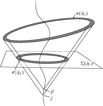
Figure 1: The emitted part propagates along the future light cone without losing energy.

By assuming $\nabla_{\mu}{T_{\rm rad}}^{\mu\nu}=0$, we obtain, by using Eq. (1),

$$E_{{\rm K}[\sigma(\tilde{\eta}_{1})]{\rm rad}}-E_{{\rm K}[\sigma(\tilde{\eta}_{2})]{\rm rad}}$$

$$\hskip 62.59596pt=\int_{L[\tilde{\eta_{1}},\tilde{\eta_{2}}]}\tilde{n}_{\mu}X_{\nu}{T_{\rm rad}}^{\mu\nu}\mbox{\boldmath$\widetilde{\epsilon}$}+\int_{L^{\prime}[\tilde{\eta_{1}},\tilde{\eta_{2}}]}\tilde{n}_{\mu}X_{\nu}{T_{\rm rad}}^{\mu\nu}\mbox{\boldmath$\widetilde{\epsilon}$},$$ (8)

where $L[\tilde{\eta_{1}},\tilde{\eta_{2}}]$ and $L^{\prime}[\tilde{\eta_{1}},\tilde{\eta_{2}}]$ are the portions of $L$ and $L^{\prime}$ that are bounded by the surfaces $\tilde{\eta}=\tilde{\eta_{1}}$ and $\tilde{\eta}=\tilde{\eta_{2}}$ ($\tilde{\eta_{1}}<\tilde{\eta_{2}}$). Then we may adopt the mathematical expression of condition 2

$$\nabla_{\mu}{T_{\rm rad}}^{\mu\nu} = 0\ \ \ {\rm and}\ \ \ \hat{n}_{\mu}X_{\nu}{T_{\rm rad}}^{\mu\nu}=0$$ (9)

($\hat{n}_{\mu}$ is a null vector which is orthogonal to $L$ or $L^{\prime}$), which is a more restricted expression than Eq. (7).

The bound part of the energy-momentum tensor

$${T_{\rm bound}}^{\mu\nu} = {T_{\rm ret}}^{\mu\nu}-{T_{\rm rad}}^{\mu\nu},$$ (10)

where ${T_{\rm ret}}^{\mu\nu}$ is the total energy-momentum tensor of retarded fields, consists of the contribution of the pure bound fields and the contribution of the interference between bound fields and radiation fields $[$see the definition of ${T_{{\rm I}}}^{\mu\nu}$ in Ref. [2] or Eq. (41) in the present paper$]$. The energy of the bound part $E_{{\rm K}[\sigma]{\rm bound}}$ in the region $\sigma$ can also be expressed as

$$E_{{\rm K}[\sigma]{\rm bound}} = -\int_{\sigma}n_{\mu}X_{\nu}{T_{\rm bound}}^{\mu\nu}\mbox{\boldmath$\widetilde{\epsilon}$},$$ (11)

then condition 3 is expressed as

$$\lim_{\tilde{\eta}\rightarrow\infty}E_{{\rm K}[\sigma(\tilde{\eta})]{\rm bound}} = 0.$$ (12)

The part which satisfies condition 3 can be interpreted as not escaping to the region infinitely separated from the charge, so we may regard this part as that “bound to the charge”. Now, we write the total energy of the retarded fields as $E_{{\rm K}[\sigma]{\rm ret}}$. Then, with the relation $E_{{\rm K}[\sigma]{\rm rad}}=E_{{\rm K}[\sigma]{\rm ret}}-E_{{\rm K}[\sigma]{\rm bound}}$ and with Eqs. (7) and (12), we find

$$E_{{\rm K}[\sigma]{\rm rad}} = \lim_{\tilde{\eta}\rightarrow\infty}E_{{\rm K}[\sigma(\tilde{\eta})]{\rm rad}}=\lim_{\tilde{\eta}\rightarrow\infty}E_{{\rm K}[\sigma(\tilde{\eta})]{\rm ret}}.$$ (13)

In the following, we seek radiation fields that satisfy conditions 1 and 2 by generalizing the reasoning of Teitelboim for the acceleration fields $[$presented from Eq. (2$\cdot$1) to Eq. (2$\cdot$11) in Ref. [2]$]$. We here note that condition 1 might not be valid in the case of general stationary frames. However, the consideration given below should be useful to examine the identification of radiation in the Rindler frame in a more general context.

For a point $p$ (with coordinate value $x^{\mu}$), a retarded point $\bar{p}$ (with coordinate value $\bar{x}^{\mu}$) is defined as the point on the worldline of the charge that satisfies the condition

$$R^{\mu} = x^{\mu}-\bar{x}^{\mu},$$ (14)

$$R^{\mu}R_{\mu} = 0$$ (15)

$$x^{t} > \bar{x}^{t}$$

expressed in an inertial frame $(t,x,y,z)$. Here we note that the definition of $R^{\mu}$ in Eq. (14) is invariant under Lorentz transformations, but it is not invariant under general coordinate transformations. Therefore, we express the equations only in inertial frames if the equations include the notation $R^{\mu}$ explicitly, unless otherwise stated.

For an arbitrary vector $\lambda^{\mu}$ at the retarded point $\bar{p}$, we define a field

$$f^{\mu\nu}(x) = \frac{e}{R^{3}}(\lambda^{\alpha}R_{\alpha})[v^{\mu}R^{\nu}-R^{\mu}v^{\nu}]+\frac{e}{R^{2}}[\lambda^{\mu}R^{\nu}-R^{\mu}\lambda^{\nu}],$$ (16)

where $v^{\mu}$ is evaluated at the retarded point $\bar{p}$, and we set $R=-v^{\mu}R_{\mu}$. Here, $f^{\mu\nu}$ is invariant with respect to the transformation $\lambda^{\mu}\rightarrow\lambda^{\mu}+lv^{\mu}$ (where $l$ is an arbitrary factor). Hence, by using ${\lambda_{\perp}}^{\mu}\equiv h^{\mu}_{\ \nu}\lambda^{\nu}$ (where $h^{\mu}_{\ \nu}=\delta^{\mu}_{\ \nu}+v^{\mu}v_{\nu}$ is the projector on the plane orthogonal to $v^{\mu}$), we can rewrite the field as

$$f^{\mu\nu}(x) = \frac{e}{R^{3}}({\lambda_{\perp}}^{\alpha}R_{\alpha})[v^{\mu}R^{\nu}-R^{\mu}v^{\nu}]+\frac{e}{R^{2}}[{\lambda_{\perp}}^{\mu}R^{\nu}-R^{\mu}{\lambda_{\perp}}^{\nu}].$$ (17)

Taking the partial derivative of $\bar{x}^{\mu}$ with respect to $x^{\nu}$ gives

$$\partial_{\nu}\bar{x}^{\mu} = v^{\mu}\partial_{\nu}\tau,$$ (18)

where $\tau$ is the proper time of the charge. From Eq. (18), we obtain

$$0 = \partial_{\mu}(R^{\alpha}R_{\alpha})=2[R_{\mu}+R(\partial_{\mu}\tau)],$$ (19)

so that

$$\partial_{\mu}\tau = -\frac{R_{\mu}}{R}.$$ (20)

Using this equation, we find

$$\partial_{\mu}R^{\nu} = \delta^{\nu}_{\ \mu}-\partial_{\mu}\bar{x}^{\nu}=\delta^{\nu}_{\ \mu}-v^{\nu}\partial_{\mu}\tau=\delta^{\nu}_{\ \mu}+\frac{v^{\nu}R_{\mu}}{R},$$ (21)

$$\partial_{\mu}R = \frac{1+a^{\alpha}R_{\alpha}}{R}R_{\mu}-v_{\mu},$$ (22)

$$\partial_{\mu}\lambda^{\nu} = (\partial_{\mu}\tau)\partial_{\tau}\lambda^{\nu}=-\frac{R_{\mu}(\partial_{\tau}\lambda^{\nu})}{R}.$$ (23)

Using Eqs. (21), (22) and (23), we obtain the equations of the field $f^{\mu\nu}$ off the worldline of the charge,

$$\partial_{[\lambda}f_{\mu\nu]} = 0,$$ (24)

$$\partial_{\mu}f^{\mu\nu} = -\frac{2e}{R^{4}}({\lambda_{\perp}}^{\alpha}R_{\alpha})R^{\nu}.$$ (25)

The energy-momentum tensor of the field $f^{\mu\nu}$ is given in the form

$$t^{\mu\nu} = \frac{1}{4\pi}\left[f^{\mu\alpha}f_{\alpha}^{\ \nu}+\frac{1}{4}g^{\mu\nu}f_{\alpha\beta}f^{\alpha\beta}\right].$$ (26)

With Eq. (24) and $f_{\mu\nu}=-f_{\nu\mu}$, we find

$$\partial_{\mu}t^{\mu\nu} = \frac{1}{4\pi}f^{\alpha\nu}(\partial_{\mu}f^{\mu}_{\ \alpha}).$$ (27)

Substituting Eqs. (16) and (25) into the above equation, we obtain the conservation law $\partial_{\mu}t^{\mu\nu}=0$ off the worldline. This result can be rewritten in general curvilinear coordinates with the covariant derivative:

$$\nabla_{\mu}t^{\mu\nu} = 0.$$ (28)

Substituting Eq. (17) into (26) and using ${\lambda_{\perp}}^{\alpha}v_{\alpha}=0$, we obtain

$$t^{\mu\nu} = \frac{e^{2}}{4\pi R^{6}}[({\lambda_{\perp}}^{\alpha}R_{\alpha})^{2}-R^{2}({\lambda_{\perp}}^{\alpha}{\lambda_{\perp}}_{\alpha})]R^{\mu}R^{\nu}.$$ (29)

From Eq. (28) and by noting $\hat{n}^{\mu}\propto R^{\mu}$ and $t^{\mu\nu}\propto R^{\mu}R^{\nu}$, we find that $t^{\mu\nu}$ satisfies Eq. (9). Therefore the field $f^{\mu\nu}$ defined in the stationary frame generated by an arbitrary Killing field satisfies condition 2. If we choose $\lambda^{\mu}$ so that ${\lambda_{\perp}}^{\mu}=0$ for the motion of the charge fixed in the frame, the field satisfies condition 1 also. For example, with the value $u^{\mu}$ at the point $\bar{p}$ of the 4-velocity $\tilde{u}^{\mu}=(-X^{\alpha}X_{\alpha})^{-1/2}X^{\mu}$ of an observer fixed in the frame, and with the value $g^{\mu}$ at the point $\bar{p}$ of the 4-acceleration $\tilde{g}^{\mu}=\tilde{u}^{\alpha}\nabla_{\alpha}\tilde{u}^{\mu}$, we can choose $\lambda^{\mu}$ in the form

$$\lambda^{\mu} = a^{\mu}-g^{\mu}-ku^{\mu},$$ (30)

where $k$ is an arbitrary scalar at the point $\bar{p}$. In this case, we find that ${\lambda_{\perp}}^{\mu}=0$ for a charge fixed in the frame ($v^{\mu}=u^{\mu}$, $a^{\mu}=g^{\mu}$), and therefore the field $f^{\mu\nu}$ with $\lambda^{\mu}$ defined as Eq. (30) satisfies conditions 1 and 2 which are required for the proper definition of the radiation fields. Thus we find that, for any stationary frame, there are several possible ways to define radiation fields that satisfy conditions 1 and 2 (at least, one can choose the form of $k$ freely).

2.3 Bound and radiation fields in the Rindler frame

In this subsection, we identify the radiation fields and bound fields in the Rindler frame by using the results of previous subsection, and with this identification, we split the energy-momentum tensor into the emitted part and bound part.

For an inertial frame $(t,x,y,z)$, the Rindler frame $(\eta,x,y,\xi)$ (see Section 4.5 in Ref. [10]) is defined as

$$t = \xi\sinh\eta,$$

$$z = \xi\cosh\eta,$$ (31)

where $-\infty<\eta<\infty$, $0<\xi<\infty$. (The Rindler frame can also be defined in the region $-\infty<\xi<0$, but we consider $\xi>0$ for simplicity.) In this case, the Rindler frame covers the region with $|t|<z$ in Minkowski spacetime. The metric in the Rindler frame is given as

$$ds^{2} = -\xi^{2}d\eta^{2}+dx^{2}+dy^{2}+d\xi^{2}.$$ (32)

Since the metric is independent of time $\eta$, there are Killing fields $X=\nu\partial_{\eta}$ ($\nu$ is an arbitrary constant) proportional to $\partial_{\eta}$. We write the energy defined by the Killing fields $\nu\partial_{\eta}$ as $E_{\rm R}$.

An observer fixed in the Rindler frame (with the trajectory where $x$ and $y$ are fixed, and $\xi=\xi_{0}=[{\rm constant}]$) is called a Rindler observer. The 4-velocity and 4-acceleration of the observer are $\tilde{u}^{\mu}=(-X^{\alpha}X_{\alpha})^{-1/2}X^{\mu}$ and $\tilde{g}^{\mu}=\tilde{u}^{\alpha}\nabla_{\alpha}\tilde{u}^{\mu}$, and the worldline is expressed as a hyperbola, $z^{2}-t^{2}={\xi_{0}}^{2}$, in the inertial frame. Since the Rindler observer moves in a fixed direction with constant acceleration $\sqrt{\tilde{g}^{\mu}\tilde{g}_{\mu}}={\xi_{0}}^{-1}$, the Rindler frame is interpreted as a uniformly accelerated frame. The region $h^{+}[t-z=0\ (\eta\rightarrow\infty,\ \xi\rightarrow 0)]$ is interpreted as the future event horizon of the Rindler frame, because the Rindler observer cannot see events beyond the region $h^{+}$. The region $h^{-}[t+z=0\ (\eta\rightarrow-\infty,\ \xi\rightarrow 0)]$ is also interpreted as the past event horizon (see Fig. 2).

If the emitted part and bound part satisfy conditions 2 and 3, we can evaluate the radiation power of the charge by using Eq. (13). Then, let us calculate $E_{{\rm R}[\sigma(\eta\rightarrow\infty)]{\rm ret}}$. First we split the energy-momentum tensor ${T_{\rm ret}}^{\mu\nu}$ into the part ${T_{{\rm I},{\rm I}}}^{\mu\nu}$, which is independent of $a^{\mu}$, the part ${T_{{\rm I},{\rm II}}}^{\mu\nu}$, which is linear in $a^{\mu}$, and the part ${T_{{\rm II},{\rm II}}}^{\mu\nu}$, which is quadratic in $a^{\mu}$ $[$ see Eqs. (2.7a) – (2.7c) in Ref. [2] or see Eq. (114) in this paper$]$, and evaluate the contributions to the parts of $E_{{\rm R}[\sigma(\eta\rightarrow\infty)]{\rm ret}}$ due to ${T_{{\rm I},{\rm I}}}^{\mu\nu}$, ${T_{{\rm I},{\rm II}}}^{\mu\nu}$ and ${T_{{\rm II},{\rm II}}}^{\mu\nu}$, respectively. Explicit calculations are given in Appendices A and B, and we note here only the results.

The contribution independent of $a^{\mu}$ is

$$\lim_{\eta\rightarrow\infty}E_{{\rm R}[\sigma(\eta)]{\rm I},{\rm I}} = -\lim_{\eta\rightarrow\infty}\int_{\sigma(\eta)}n_{\mu}X_{\nu}{T_{{\rm I},{\rm I}}}^{\mu\nu}\mbox{\boldmath$\widetilde{\epsilon}$}$$ (33)

$$= \frac{2e^{2}}{3}[v_{\mu}(\sqrt{g^{\beta}g_{\beta}}u^{\mu}+g^{\mu})]^{2}(-\bar{X}^{\alpha}v_{\alpha})d\tau,$$

the contribution linear in $a^{\mu}$ is

$$\lim_{\eta\rightarrow\infty}E_{{\rm R}[\sigma(\eta)]{\rm I},{\rm II}} = -\lim_{\eta\rightarrow\infty}\int_{\sigma(\eta)}n_{\mu}X_{\nu}{T_{{\rm I},{\rm II}}}^{\mu\nu}\mbox{\boldmath$\widetilde{\epsilon}$}$$ (34)

$$= -\frac{4e^{2}}{3}a_{\mu}(\sqrt{g^{\beta}g_{\beta}}u^{\mu}+g^{\mu})(-\bar{X}^{\alpha}v_{\alpha})d\tau,$$

and the contribution quadratic in $a^{\mu}$ is

$$\lim_{\eta\rightarrow\infty}E_{{\rm R}[\sigma(\eta)]{\rm II},{\rm II}} = -\lim_{\eta\rightarrow\infty}\int_{\sigma(\eta)}n_{\mu}X_{\nu}{T_{{\rm II},{\rm II}}}^{\mu\nu}\mbox{\boldmath$\widetilde{\epsilon}$}$$ (35)

$$= \frac{2e^{2}}{3}a^{\mu}a_{\mu}(-\bar{X}^{\alpha}v_{\alpha})d\tau,$$

where $u^{\mu}$, $g^{\mu}$ and $\bar{X}^{\mu}$ are the values of $\tilde{u}^{\mu}$, $\tilde{g}^{\mu}$ and $X^{\mu}$ at the retarded point $\bar{p}$, and $d\tau$ is the proper time interval of the charge between $\bar{p}$ and $\bar{p}^{\prime}$. We also note that $-\bar{X}^{\alpha}v_{\alpha}>0$.

We would like to point out here that the above results explicitly show that the splitting of the energy-momentum tensor into the parts ${\rm I}$ and ${\rm II}$ performed by Teitelboim does not satisfy conditions 1 and 3 in the Rindler frame. On the other hand, condition 2 remains valid, because part ${\rm II}$ is produced by the field $f^{\mu\nu}$ with ${\lambda_{\perp}}^{\mu}=a^{\mu}$.

By summing up these contributions, we obtain the energy of the total electromagnetic field in the region $\sigma(\eta\rightarrow\infty)$ as

$$\lim_{\eta\rightarrow\infty}E_{{\rm R}[\sigma(\eta)]{\rm ret}} = \lim_{\eta\rightarrow\infty}[E_{{\rm R}[\sigma(\eta)]{\rm I},{\rm I}}+E_{{\rm R}[\sigma(\eta)]{\rm I},{\rm II}}+E_{{\rm R}[\sigma(\eta)]{\rm II},{\rm II}}]$$ (36)

$$= \frac{2e^{2}}{3}\alpha^{\mu}\alpha_{\mu}(-\bar{X}^{\beta}v_{\beta})d\tau.$$

Here

$$\alpha^{\mu} = h^{\mu}_{\ \nu}[a^{\nu}-w^{\nu}],$$

$$w^{\mu} = (g^{\alpha}g_{\alpha})^{1/2}u^{\mu}+g^{\mu},$$ (37)

where $w^{\mu}$ is a null vector:

$$w^{\mu}w_{\mu} = 0.$$ (38)

We can write $\alpha^{\mu}=a^{\mu}-{w_{\perp}}^{\mu}$ with the notation ${w_{\perp}}^{\mu}=h^{\mu}_{\ \nu}w^{\nu}$. At the instant that the charge is at rest in the Rindler frame ($v^{\mu}=u^{\mu}$), we find $\alpha^{\mu}=a^{\mu}-g^{\mu}$. Hence $\alpha^{\mu}$ can be interpreted as the acceleration of the charge relative to the Rindler frame.

Equation (36) resembles the Larmor formula in inertial frames,

$$\lim_{t\rightarrow\infty}E_{{\rm M}[\sigma(t)]{\rm ret}} = \frac{2e^{2}}{3}a^{\mu}a_{\mu}(-\bar{\partial_{t}}^{\alpha}v_{\alpha})d\tau,$$ (39)

where $E_{\rm M}$ is the energy defined with respect to the Killing vector field $\partial_{t}$ of the inertial frame, $\sigma(t)$ is the intersection of simultaneous surface in the inertial frame with $\Delta L$. By replacing $\partial_{t}$ and $a^{\mu}$ with $X^{\mu}$ and $\alpha^{\mu}$ in Eq. (39), we again obtain the expression in Eq. (36). In analogy to the fact that the radiation fields ${\rm II}$ are linear in $a^{\mu}$ and the bound fields ${\rm I}$ are independent of $a^{\mu}$ in an inertial frame, we split the retarded fields into a part that is linear in $\alpha^{\mu}$ and a part that is independent of $\alpha^{\mu}$:

$${F_{\rm ret}}^{\mu\nu} = {F_{\ \widetilde{\rm I}}}^{\mu\nu}+{F_{\ \widetilde{\rm II}}}^{\mu\nu},$$

$${F_{\ \widetilde{\rm I}}}^{\mu\nu} = \frac{e}{R^{3}}(1+{w_{\perp}}^{\alpha}R_{\alpha})[v^{\mu}R^{\nu}-R^{\mu}v^{\nu}]+\frac{e}{R^{2}}[{w_{\perp}}^{\mu}R^{\nu}-R^{\mu}{w_{\perp}}^{\nu}],$$

$${F_{\ \widetilde{\rm II}}}^{\mu\nu} = \frac{e}{R^{3}}(\alpha^{\alpha}R_{\alpha})[v^{\mu}R^{\nu}-R^{\mu}v^{\nu}]+\frac{e}{R^{2}}[\alpha^{\mu}R^{\nu}-R^{\mu}\alpha^{\nu}].$$ (40)

This splitting of the field causes a splitting of the energy-momentum tensor into two parts:

$${T_{\rm ret}}^{\mu\nu} = {T_{\ \widetilde{\rm I}}}^{\mu\nu}+{T_{\ \widetilde{\rm II}}}^{\mu\nu},$$

$${T_{\ \widetilde{\rm I}}}^{\mu\nu} = \frac{1}{4\pi}\left[{F_{\ \widetilde{\rm I}}}^{\mu\alpha}{F_{\ \widetilde{\rm I}}}_{\alpha}^{\ \nu}+\frac{1}{4}g^{\mu\nu}{F_{\ \widetilde{\rm I}}}_{\alpha\beta}{F_{\ \widetilde{\rm I}}}^{\alpha\beta}\right.$$

$$\hskip 22.76228pt\left.+{F_{\ \widetilde{\rm I}}}^{\mu\alpha}{F_{\ \widetilde{\rm II}}}_{\alpha}^{\ \nu}+{F_{\ \widetilde{\rm II}}}^{\mu\alpha}{F_{\ \widetilde{\rm I}}}_{\alpha}^{\ \nu}+\frac{1}{2}g^{\mu\nu}{F_{\ \widetilde{\rm I}}}_{\alpha\beta}{F_{\ \widetilde{\rm II}}}^{\alpha\beta}\right],$$

$${T_{\ \widetilde{\rm II}}}^{\mu\nu} = \frac{1}{4\pi}\left[{F_{\ \widetilde{\rm II}}}^{\mu\alpha}{F_{\ \widetilde{\rm II}}}_{\alpha}^{\ \nu}+\frac{1}{4}g^{\mu\nu}{F_{\ \widetilde{\rm II}}}_{\alpha\beta}{F_{\ \widetilde{\rm II}}}^{\alpha\beta}\right].$$ (41)

Since ${F_{\ \widetilde{\rm II}}}^{\mu\nu}$ corresponds to the field $f^{\mu\nu}$ with $\lambda^{\mu}=a^{\mu}-w^{\mu}$, and since $a^{\mu}-w^{\mu}$ satisfies Eq. (30), ${F_{\ \widetilde{\rm II}}}^{\mu\nu}$ can be regarded as the radiation fields that satisfy the conditions 1 and 2. By using the results of previous subsection, we find that the following equations are valid off the world line of the charge:

$$\nabla_{[\lambda}{F_{\ \widetilde{\rm II}}}_{\mu\nu]} = 0,$$ (42)

$$\nabla_{\mu}{F_{\ \widetilde{\rm II}}}^{\mu\nu} = -\frac{2e}{R^{4}}(\alpha^{\mu}R_{\mu})R^{\nu},$$ (43)

$$\nabla_{\mu}{T_{\ \widetilde{\rm II}}}^{\mu\nu} = 0,$$ (44)

$${T_{\ \widetilde{\rm II}}}^{\mu\nu} = \frac{e^{2}}{4\pi R^{6}}[(\alpha^{\beta}R_{\beta})^{2}-R^{2}(\alpha^{\beta}\alpha_{\beta})]R^{\mu}R^{\nu}.$$ (45)

From the equations concerning the total retarded fields and their energy-momentum tensor $\nabla_{[\lambda}{F_{\rm ret}}_{\mu\nu]}=0$, $\nabla_{\mu}{F_{\rm ret}}^{\mu\nu}=0$ and $\nabla_{\mu}{T_{\rm ret}}^{\mu\nu}=0$, and from the equations concerning part $\widetilde{\rm II}$ above, we find that ${F_{\ \widetilde{\rm I}}}^{\mu\nu}$ and ${T_{\ \widetilde{\rm I}}}^{\mu\nu}$ satisfy the following equations off the world line of the charge:

$$\nabla_{[\lambda}{F_{\ \widetilde{\rm I}}}_{\mu\nu]} = 0,$$ (46)

$$\nabla_{\mu}{F_{\ \widetilde{\rm I}}}^{\mu\nu} = \frac{2e}{R^{4}}(\alpha^{\mu}R_{\mu})R^{\nu},$$ (47)

$$\nabla_{\mu}{T_{\ \widetilde{\rm I}}}^{\mu\nu} = 0.$$ (48)

Now, from the equation

$$\lim_{\eta\rightarrow\infty}E_{{\rm R}[\sigma(\eta)]\widetilde{\rm I}} = \lim_{\eta\rightarrow\infty}E_{{\rm R}[\sigma(\eta)]{\rm ret}}-E_{{\rm R}[\sigma(\eta)]\widetilde{\rm II}}$$ (49)

and the equation

$$E_{{\rm R}[\sigma(\eta)]\widetilde{\rm II}} = \frac{2e^{2}}{3}\alpha^{\mu}\alpha_{\mu}(-\bar{X}^{\alpha}v_{\alpha})d\tau,$$ (50)

which is derived by using Eq. (45) and the calculation in the appendices (see the comment below Eq. (150) in Appenix B), we find that

$$\lim_{\eta\rightarrow\infty}E_{{\rm R}[\sigma(\eta)]\widetilde{\rm I}} = 0.$$ (51)

Therefore, part $\widetilde{\rm I}$ of the energy-momentum tensor is regarded as the bound part, which satisfies condition 3.

In conclusion, we find that part $\widetilde{\rm I}$ and part $\widetilde{\rm II}$, which are defined in Eqs. (40) and (41), can be considered as the bound part and the emitted part in the Rindler frame, respectively, in the sense that these parts satisfy the conditions 1, 2 and 3.

3 Physical implications of our identification

In this section, we investigate the implications of our identification of the emitted part and bound part in the Rindler frame given in the previous section. Although we have distinguished ${\bar{x}}^{\mu}$ from $x^{\mu}$ and $\bar{X}^{\mu}$ from $X^{\mu}$ in the previous section and Appendices A and B, we do not make a distinction between these notations in this section, because we deal with quantities only on the world line of the charge here.

3.1 Trajectory of a point charge with no radiation

In our identification of radiation fields, the charge emits radiation neither in the case that the charge is fixed to the Rindler frame, nor in the case that $\alpha^{\mu}=0$. Thus, in this subsection, we investigate the trajectory of the charge which satisfies the equation $\alpha^{\mu}=0$.

From the 4-velocity of the Rindler observer in the Rindler frame,

$$(u^{\eta},u^{x},u^{y},u^{\xi}) = (\xi^{-1},0,0,0),$$ (52)

and the non-zero components of the Christoffel symbol in the Rindler frame,

$$\Gamma^{\eta}_{\xi\eta} = \Gamma^{\eta}_{\eta\xi}=\xi^{-1},\ \ \ \ \Gamma^{\xi}_{\eta\eta}=\xi,$$ (53)

we obtain the 4-acceleration $g^{\mu}=u^{\alpha}\nabla_{\alpha}u^{\mu}$ in the Rindler frame,

$$(g^{\eta},g^{x},g^{y},g^{\xi}) = (0,0,0,\xi^{-1}).$$ (54)

Taking covariant derivatives of Eqs. (52) and (54) gives

$$v^{\mu}\nabla_{\mu}g^{\nu} = -(v\cdot g)g^{\nu}-(g\cdot g)(v\cdot u)u^{\nu},$$ (55)

$$v^{\mu}\nabla_{\mu}u^{\nu} = -(u\cdot v)g^{\nu},$$ (56)

where we use the notation $(p\cdot q)=p^{\alpha}q_{\alpha}$. Equations (55) and (56) further give

$$v^{\mu}\nabla_{\mu}\sqrt{g\cdot g} = -(v\cdot g)\sqrt{g\cdot g},$$ (57)

$$v^{\mu}\nabla_{\mu}w^{\nu} = v^{\mu}\nabla_{\mu}[\sqrt{g\cdot g}u^{\nu}+g^{\nu}]=-(v\cdot w)w^{\nu}.$$ (58)

From Eq. (58) and $v^{\mu}\nabla_{\mu}h^{\alpha}_{\ \beta}=a^{\alpha}v_{\beta}+v^{\alpha}a_{\beta}$, we find

$$v^{\mu}\nabla_{\mu}{w_{\perp}}^{\nu} = (v\cdot w)\alpha^{\nu}+v^{\nu}(a\cdot w).$$ (59)

According to the Lorentz-Dirac equations, the radiation reaction force acting on the charge is given as

$$\Gamma^{\mu} = \frac{2e^{2}}{3}[v^{\alpha}\nabla_{\alpha}a^{\mu}-v^{\mu}(a\cdot a)].$$ (60)

By using Eq. (59), we find that the radiation reaction force vanishes for a charge with motion such that $\alpha^{\mu}=0$, or $a^{\mu}={w_{\perp}}^{\mu}$:

$$\Gamma^{\mu}=0.$$ (61)

We thus find the natural result that a charge that does not radiate in the Rindler frame also does not experience a radiation reaction force. The trajectory with $\Gamma^{\mu}=0$ constitutes uniformly accelerated motion. $[$According to the discussions of Sections 5.3 and 6.11 in Ref. [11], uniformly accelerated motion is defined by the equation $v^{\lambda}\nabla_{\lambda}a^{\mu}=a^{\lambda}a_{\lambda}v^{\mu}$, which is equivalent to Eq. (61).$]$ Thus there is an inertial frame $(t^{\prime\prime},x^{\prime\prime},y^{\prime\prime},z^{\prime\prime})$ in which the trajectory $\Gamma^{\mu}=0$ represents hyperbolic motion $[$see Eq. (6$\cdot$127) in Section 6.11 of Ref. [11]$]$ given by

$$t^{\prime\prime} = \kappa^{-1}\sinh(\kappa\tau)$$

$$z^{\prime\prime} = \kappa^{-1}\cosh(\kappa\tau),$$ (62)

where $\kappa$ is the acceleration of the trajectory $\alpha^{\mu}=0$ and evaluated as

$$\kappa = \sqrt{{w_{\perp}}\cdot{w_{\perp}}}=v^{\eta}-\xi^{-1}v^{\xi}.$$ (63)

We note that, for uniformly accelerated motion $v^{\alpha}\nabla_{\alpha}a^{\mu}=a^{\alpha}a_{\alpha}v^{\mu}$, it follows that $v^{\alpha}\nabla_{\alpha}(a^{\mu}a_{\mu})=0$, so that $\kappa$ is a constant throughout the motion (see Section 6.11 in Ref. [11]).

Let us investigate the equation $a^{\mu}={w_{\perp}}^{\mu}$ by means of the Rindler coordinates. Substituting Eqs. (52) – (54) into the equation $a^{\mu}={w_{\perp}}^{\mu}$, we find the $\eta$, $\xi$, $x$ and $y$ components of the equation as

$$\frac{dv^{\eta}}{d\tau} = \xi^{-2}-\xi^{-1}v^{\xi}v^{\eta}-(v^{\eta})^{2},$$ (64)

$$\frac{dv^{\xi}}{d\tau} = \xi^{-1}+\xi^{-1}(v^{\xi})^{2}-v^{\eta}v^{\xi}-\xi(v^{\eta})^{2},$$ (65)

$$\frac{dv^{x}}{d\tau} = (\xi^{-1}v^{\xi}-v^{\eta})v^{x},$$ (66)

$$\frac{dv^{y}}{d\tau} = (\xi^{-1}v^{\xi}-v^{\eta})v^{y},$$ (67)

where $v^{\mu}=dx^{\mu}/d\tau$. In addition to these equations, we should consider the conditions $v^{\mu}v_{\mu}=-1$ and $v^{\eta}>0$. (We also consider $\xi>0$.) The former condition ensures that $\tau$ is the proper time, and the latter condition ensures that the coordinate time $\eta$ and the proper time $\tau$ are oriented in the same direction.

By using Eqs. (64) and (65), we can explicitly confirm the above statement that acceleration $\kappa$ is conserved:

$$\frac{d}{d\tau}(v^{\eta}-\xi^{-1}v^{\xi}) = 0.$$ (68)

Equation (64) can be rewritten in the form

$$\frac{1}{2}\frac{d}{d\tau}[(\xi v^{\eta})^{2}-1] = -v^{\eta}[(\xi v^{\eta})^{2}-1].$$ (69)

We express the speed of the particle in the Rindler frame as $V=\{(v^{x})^{2}+(v^{y})^{2}+(v^{\xi})^{2}\}^{1/2}$. Then we can write $V^{2}=(\xi v^{\eta})^{2}-1$ by noting $v^{\mu}v_{\mu}=-1$. Substituting this expression into Eq. (69), it follows that

$$\frac{dV}{d\eta} = -V.$$ (70)

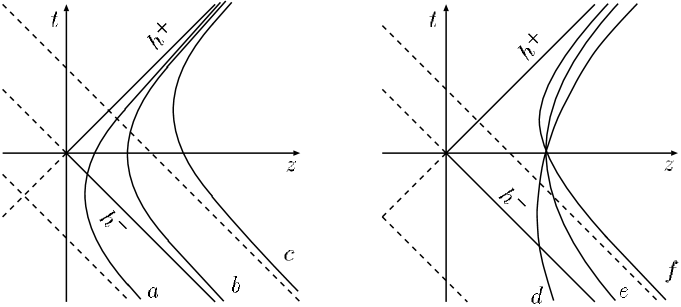
Figure 2: Trajectories given by the equation $\alpha^{\mu}=0$ are illustrated in the special case that $v^{x}=v^{y}=0$. Trajectories $a$, $b$ and $c$ experiencing the same acceleration $\kappa$ are asymptotically at rest in the Rindler frame with the same coordinate value $\xi=\kappa^{-1}$. Trajectories with velocities $v^{\xi}>0$, $v^{\xi}=0$ and $v^{\xi}<0$ are illustrated as the curves $d$, $e$ and $f$. We find that the trajectory with $v^{\xi}>0$ intersects the past event horizon $h^{-}$.

Then we find that $V\propto e^{-\eta}$ and that the speed $V$ decreases as the time $\eta$ is increased.

By integrating the set of Eqs. (68), (69), (66) and (67) , we obtain the solution of equation $a^{\mu}={w_{\perp}}^{\mu}$ (for details of the calculation, see Appendix C):

$$\sqrt{e^{2\eta}+A}=(\kappa\zeta)^{-1}e^{\kappa\tau}+B,$$ (71)

$$\xi=\zeta\left[\{(\kappa\zeta)^{-1}+Be^{-\kappa\tau}\}^{2}-Ae^{-2\kappa\tau}\right]^{1/2},$$ (72)

$$x=\beta_{x}e^{-\kappa\tau}+x_{f},$$ (73)

$$y=\beta_{y}e^{-\kappa\tau}+y_{f},$$ (74)

where the constants of integration $\kappa$, $\zeta$, $A$, $B$, $\beta_{x}$, $x_{f}$, $\beta_{y}$ and $y_{f}$ satisfy following conditions:

$$\kappa>0,\ \ \ \zeta>0$$

$$B^{2}-A\zeta^{2}+{\beta_{x}}^{2}+{\beta_{y}}^{2}=0.$$ (75)

By taking the limit $\tau\rightarrow\infty$ of this solution, we find that

$$\eta \rightarrow \kappa\tau-\frac{1}{2}\ln(\kappa\zeta),$$ (76)

$$(x,y,\xi) \rightarrow (x_{f},y_{f},\kappa^{-1}).$$ (77)

We thus see that the particle approaches a state of being at rest in the Rindler frame in the infinite future.

In conclusion $[$Eqs. (61), (70) and (77)$]$, we find that the velocity of a particle that obeys the equation $a^{\mu}={w_{\perp}}^{\mu}$ gradually decreases relative to the Rindler frame, and, in the limit $\eta\rightarrow\infty$, the particle is at rest in the Rindler frame. Also we find that the charge does not experience a radiation reaction force, which implies that there is an inertial frame in which the particle exhibits the hyperbolic motion described by Eq. (62). We illustrate the trajectories with $a^{\mu}={w_{\perp}}^{\mu}$ in the special case that $v^{x}=v^{y}=0$ in Fig. 2.

3.2 Bound electromagnetic energy in the Rindler frame

In Teitelboim’s original paper [2], the bound character of part ${\rm I}$ is strongly confirmed by showing that the 4-momentum of part ${\rm I}$ is a state function of the charge. In that paper, the 4-momentum of the part ${\rm I}$ is defined as

$${P_{{\rm I}}}^{\mu}(t) = \int_{\Sigma(t)}{T_{{\rm I}}}^{\nu\mu}n_{\nu}\mbox{\boldmath$\widetilde{\epsilon}$},$$ (78)

expressed in the inertial frame, where $\Sigma(t)$ is a space-like plane in Minkowski spacetime, and $n^{\nu}$ is a future directed unit vector normal to the plane $\Sigma(t)$. Since ${T_{{\rm I}}}^{\nu\mu}n_{\nu}$ is infinite on the world line of the charge, one integrates it over $\Sigma(t)$, except inside the sphere of small radius $\epsilon$ that surrounds the charge.

In the original paper [2], $\Sigma(t)$ is set orthogonal to the world line of the charge, and the result is $[$ Eq. (3.20) in Ref. [2]$]$

$${P_{{\rm I}}}^{\mu} = \frac{e^{2}}{2\epsilon}v^{\mu}-\frac{2e^{2}}{3}a^{\mu}.$$ (79)

Although ${T_{{\rm I}}}^{\nu\mu}$ in Eq. (78) is a retarded function, and thus ${P_{{\rm I}}}^{\mu}$ is defined by the integration over the entire history of the charge, the total integral depends only on the instantaneous state of the charge $[v^{\mu}$ and $a^{\mu}$ in Eq. (79)$]$. This noteworthy result implies that we can regard part ${\rm I}$ as bound to charge [2].

To strongly confirm the bound character of part $\widetilde{\rm I}$ in the Rindler frame, we should evaluate the total energy of $\widetilde{\rm I}$ in the Rindler frame. Although we do not explicitly evaluate the total energy here, we make a rough estimation concerning the interaction of the charge with part $\widetilde{\rm I}$ in terms of the energy defined in the Rindler frame, by using the Lorentz-Dirac equations.

The energy of a particle in a stationary frame generated by the Killing vector field $X^{\mu}$ may be written as

$$E_{\rm Kp} = -X^{\mu}v_{\mu},$$ (80)

where we assume a particle with unit mass. By using the Killing equation $\nabla_{\mu}X_{\nu}+\nabla_{\nu}X_{\mu}=0$, we obtain the rate of change of the energy of the particle per unit proper time as

$$v^{\alpha}\nabla_{\alpha}E_{\rm Kp} = -X^{\mu}(v^{\alpha}\nabla_{\alpha}v_{\mu}).$$ (81)

Of course, for a free particle ($v^{\lambda}\nabla_{\lambda}v_{\mu}=0$), $E_{\rm Kp}$ is a constant.

From the Lorentz-Dirac equations $v^{\alpha}\nabla_{\alpha}v^{\mu}={F_{\rm ext}}^{\mu}+\Gamma^{\mu}$ and Eq. (81), we can infer that the energy $\Delta W_{\rm R}$ provided by the moving charge for the electromagnetic field per proper time is $X^{\mu}\Gamma_{\mu}$. Substituting $a^{\mu}=\alpha^{\mu}+{w_{\perp}}^{\mu}$ into Eq. (60), and applying Eq. (59), we obtain

$$\frac{3}{2e^{2}}\Gamma^{\nu} = v^{\mu}\nabla_{\mu}\alpha^{\nu}+(v\cdot w)\alpha^{\nu}-v^{\nu}(\alpha\cdot w)-v^{\nu}(\alpha\cdot\alpha).$$ (82)

By noting $X^{\mu}\propto(g\cdot g)^{-1/2}u^{\mu}$, and using Eqs. (56) and (57), we get, for the Killing vector field of the Rindler frame,

$$v^{\mu}\nabla_{\mu}X^{\nu} = (v\cdot g)X^{\nu}-(X\cdot v)g^{\nu}$$ (83)

$$= (v\cdot w)X^{\nu}-(X\cdot v)w^{\nu}.$$

From Eqs. (82) and (83), it follows that

$$\Delta W_{\rm R} = X^{\mu}\Gamma_{\mu}$$ (84)

$$= \frac{2e^{2}}{3}v^{\mu}\nabla_{\mu}(X\cdot\alpha)-\frac{2e^{2}}{3}(X^{\alpha}v_{\alpha})\alpha^{\mu}\alpha_{\mu}.$$

According to Eq. (50), the second term on the right-hand side of this equation, $-(2e^{2}/3)(X^{\alpha}v_{\alpha})\alpha^{\mu}\alpha_{\mu}$, is interpreted as the contribution to the emitted part $\widetilde{\rm II}$, so that we can infer that the contribution to the bound part $\widetilde{\rm I}$ is

$$\frac{2e^{2}}{3}v^{\mu}\nabla_{\mu}(X\cdot\alpha) = \frac{d}{d\tau}\left[\frac{2e^{2}}{3}X^{\mu}\alpha_{\mu}\right].$$ (85)

Compared with the calculation concerning part ${\rm I}$ performed by Teitelboim, this result is analogous to Eq. (3.18) in Ref. [2]. The fact that Eq. (85) has an integrable form implies that the Rindler energy of part $\widetilde{\rm I}$ would include the contribution $(2e^{2}/3)X^{\mu}\alpha_{\mu}$, which is analogous to the second term (Schott term) on the right-hand side of Eq. (79).

4 Discussion

In the Rindler frame, we have identified the emitted and bound parts of the energy-momentum tensor of the retarded fields, in accordance with the three conditions introduced in § 2.2. Equations derived here in the Rindler frame are regarded as natural extensions of equations in the inertial frame derived by Teitelboim (with the replacement of $\bar{X}$ for $\bar{\partial}_{t}$ and $\alpha^{\mu}$ for $a^{\mu}$).

In application of our work to general accelerated frames with Killing fields other than the Rindler frame, condition 2 would remain valid, because this condition is crucial to define radiation. Conditions 1 and 3, however, may be replaced with other conditions. To examine the applicability of condition 1 in general accelerated frames, it might be effective to examine whether the Poynting flux generated by a charge fixed in the frame is zero, as seen by an observer fixed in the same frame. Also, as mentioned in § 3.2, to identify the bound part of the Maxwell tensor, it is important to determine whether the total energy of this part is a state function of the charge. This requirement, which provides a physical picture for the definition of the bound part, seems to be more essential than the formal requirment of condition 3.

In our result, a charge in the Rindler frame radiates neither in the case that the charge is fixed in the Rindler frame, nor in the case that the charge follows the trajectory $\alpha^{\mu}=0$. There are studies concerning classical radiation in the Rindler frame, where the non-existence of radiation from the charge fixed in the Rindler frame is discussed, but the non-existence of radiation from the charge with other trajectories has not been discussed (or, at least, the author does not know of such studies). Therefore, this might provide a new point of view in the study of radiation in the Rindler frame.

There is an old paradox of classical electrodynamics concerning the radiation from a charge with uniformly accelerated motion [5, 6]. We now apply our result in the Rindler frame to this problem. It seems that this paradox has been discussed in subtly distinct situations or points of view in the literature. Here we restrict our attention to the following problem. Let us compare the situation in which a charge exhibits uniformly accelerated motion with the situation in which a charge is fixed in a static gravitational field. These two situations might be distinguished by examining the radiation from the charge, because, in the former case, the charge radiates according to the Larmor formula, and in the latter case it does not radiate due to the energy conservation. However, this conclusion seems to contradict the principle of equivalence, which asserts that one cannot distinguish an accelerated frame from a gravitational field. This paradox may be resolved by noting that the concept (or detection) of radiation depends on the observer. In the above described situation, radiation in the gravitational field is defined with respect to the observer supported in that field. Therefore one should compare the radiation defined by this observer with the radiation defined by the observer fixed in the accelerated frame. In this case, the Larmor formula is not applicable, because this formula defines radiation with respect to an inertial observer. As mentioned above, in the literature, it has been asserted that an observer fixed in the Rindler frame does not detect radiation from a charge fixed in the same frame because of the vanishing of the Poynting flux [6].

The following four gedanken experiments are often disscussed in the context of the observer dependence of the concept of radiation. Let us consider whether the observer detects radiation from the charge in the following four situations:

1. a charge fixed in an inertial frame, with an observer fixed in the same frame,

2. a charge in uniform acceleration, with an observer fixed in an inertial frame,

3. a charge in inertial motion, with an observer fixed in a uniformly accelerated frame,

4. a charge fixed in a uniformly accelerated frame, with an observer fixed in the same frame.
   

In cases A and B, we can use the definition of radiation given by Rohrlich and Teitelboim (Larmor formula), with the result that the radiation is detected in case B, but not detected in case A. In cases C and D, where the observer experiences uniformly accelerated motion, it would be appropriate to use the definition of radiation in the Rindler frame $[$Eq. (36) or Eq. (50)$]$. Then, it is concluded that the observer does not detect radiation in case D, because our identification of radiation satisfies condition 1, but does detect radiation in case C, because $\alpha^{\mu}\neq 0$.

Our work in the Rindler frame provides a picture in which the concept of radiation depends on the observer. We here note that there is an analogous situation in quantum field theory, which is called ‘Hawking effect’ or ‘Unruh effect’ [10, 12]. This effect consists of the prediction in quantum field theory that a uniformly accelerated observer in a vacuum perceives a thermal bath of particles with temperature proportional to his acceleration. This prediction provides the physical interpretation that an observer experiencing inertial motion and an observer experiencing uniform acceleration do not agree on the number of particles observed. Therefore we find that, in the quantum case, the concept of particles depends on the observer, analogous to the observer dependence of the concept of radiation in classical theory. It might be interesting to study classical radiation in accelerated frames and general curved spacetimes to investigate the connection to quantum theory [14].

Appendix A Radiation formula in the Rindler frame

In this appendix, we derive Eqs. (33) – (35), to obtain the radiation formula (36) in the Rindler frame. First, we calculate the Rindler energy ${E_{\rm R}}^{\flat}$ with the the Killing vector field $X=\partial_{\eta}\equiv X^{\flat}$. Then we obtain the Rindler energy $E_{\rm R}$ with the Killing vector field $X=\nu\partial_{\eta}$ by multiplying ${E_{\rm R}}^{\flat}$ by $\nu$.

We introduce cylindrical coordinates $(\xi,\rho,\varphi)$ in a simultaneous plane $\eta=[{\rm constant}]$ in the Rindler frame. $\rho$ and $\varphi$ are defined as

$$x-\bar{x} = \rho\cos\varphi,$$ (86)

$$y-\bar{y} = \rho\sin\varphi.$$ (87)

Here we assume that $\bar{x}$ and $\bar{y}$ are the coordinates of the point $\bar{p}$ fixed on the world line of the charge, at which the radiation we evaluate is emitted. With the notation used in Eqs. (86) and (87), $x$ and $y$ are defined throughout the region $\eta=[{\rm constant}]$, and $\bar{x}$ and $\bar{y}$ are not retarded functions of $x$ and $y$. The volume element in the region $\eta=[{\rm constant}]$ is expressed as $\mbox{\boldmath$\widetilde{\epsilon}$}=\rho d\rho d\phi d\xi$.

In our cylindrical coordinates, ${E_{\rm R}}^{\flat}$ is written

$$\lim_{\eta\rightarrow\infty}E_{{\rm R}[\sigma(\eta)]}^{\ \flat} = -\lim_{\eta\rightarrow\infty}\int_{\sigma(\eta)}n_{\mu}{X^{\flat}}_{\nu}T^{\mu\nu}\mbox{\boldmath$\widetilde{\epsilon}$}$$ (88)

$$= -\lim_{\eta\rightarrow\infty}\int_{0}^{2\pi}d\varphi\int_{\xi_{\rm min}}^{\xi_{\rm max}}d\xi|\rho d\rho|\xi^{3}T^{\eta\eta},$$

where $\xi_{\rm min}$ and $\xi_{\rm max}$ are, respectively, the minimum value and the maximum value of $\xi$ in the region $\sigma(\eta)$. Let us rewrite $\rho d\rho$ in Eq. (88) with respect to the proper time $d\tau$ between the point $\bar{p}$ (with coordinate values $\bar{x}^{\mu}$) and the point $\bar{p}^{\prime}$ (with coordinate values $\bar{x}^{\prime\mu}$). Let us assume that the points $x^{\mu}$ and $x^{\prime\mu}$ are, respectively, the points in the future light cones with apexes $\bar{x}^{\mu}$ and $\bar{x}^{\prime\mu}$, where $\eta=\eta^{\prime},\ \ \xi=\xi^{\prime},\ \ \varphi=\varphi^{\prime}$. With the definitions $R^{\mu}=x^{\mu}-\bar{x}^{\mu}$ and $R^{\prime\mu}=x^{\prime\mu}-\bar{x}^{\prime\mu}$, it follows that

$$R^{\mu}R_{\mu} = \xi^{2}+\bar{\xi}^{2}-2\xi\bar{\xi}\cosh(\eta-\bar{\eta})+\rho^{2},$$ (89)

$$R^{\prime\mu}R^{\prime}_{\mu} = \xi^{2}+\bar{\xi}^{\prime 2}-2\xi\bar{\xi}^{\prime}\cosh(\eta-\bar{\eta}^{\prime})+(x^{\prime}-\bar{x}^{\prime})^{2}+(y^{\prime}-\bar{y}^{\prime})^{2}.$$ (90)

Substituting $\bar{x}^{\prime\mu}=\bar{x}^{\mu}+v^{\mu}d\tau$ into Eq. (90), and ignoring contributions of higher order in $d\tau$, we obtain

$$R^{\prime\mu}R^{\prime}_{\mu} = R^{\mu}R_{\mu}+\rho^{\prime 2}-\rho^{2}+2Rd\tau,$$ (91)

where we have used Eq. (89) and

$$R = -R^{\mu}v_{\mu}$$ (92)

$$= [\bar{\xi}-\xi\cosh(\eta-\bar{\eta})]v^{\xi}+\xi\bar{\xi}\sinh(\eta-\bar{\eta})v^{\eta}-(x-\bar{x})v^{x}-(y-\bar{y})v^{y}.$$

By noting $R^{\mu}R_{\mu}=R^{\prime\mu}R^{\prime}_{\mu}=0$ and $\rho^{\prime 2}-\rho^{2}=2\rho d\rho$, we find that Eq. (91) gives

$$\rho d\rho=-Rd\tau.$$ (93)

From Eq. (89) and $R^{\mu}R_{\mu}=0$, it follows that

$$(x-\bar{x})^{2}+(y-\bar{y})^{2}+(\xi-\bar{\xi}\widehat{c})^{2} = \bar{\xi}^{2}\widehat{s}^{2},$$ (94)

where we have used the definitions

$$\widehat{c} = \cosh(\eta-\bar{\eta}),$$ (95)

$$\widehat{s} = \sinh(\eta-\bar{\eta}).$$ (96)

According to Eq. (94), we find that the region of integration in Eq. (88) is the spherical shell with radius $\bar{\xi}\widehat{s}$ centered at the point $(\bar{x},\bar{y},\bar{\xi}\widehat{c})$ in the space $(x,y,\xi)$. We refer to this spherical shell as $S$.

Here we introduce the new cylindrical coordinates $(R^{*},\mu,\theta)$ in the region $\eta=[{\rm constant}]$. $R^{*}$ is defined as

$$R^{*} = [\bar{\xi}-\xi\widehat{c}]v^{\xi}+\xi\bar{\xi}\widehat{s}v^{\eta}-(x-\bar{x})v^{x}-(y-\bar{y})v^{y},$$ (97)

where $\bar{\eta}$, $\bar{\xi}$, $\bar{x}$, $\bar{y}$, $v^{\eta}$, $v^{\xi}$, $v^{x}$ and $v^{y}$ are evaluated at the fixed point $\bar{p}$, so that these are constant throughout the region $\eta=[{\rm constant}]$. (Of course, $R$ is also defined in the same form as in Eq. (97), although, in this case, $\bar{x}^{\mu}$ and $v^{\mu}$ are the retarded functions of $x^{\mu}$, so that these are not constants.) Now we introduce the vectors

$${\bf P} = -(Y^{x}_{\ \ \mu}|_{p}v^{\mu}|_{\bar{p}},Y^{y}_{\ \ \mu}|_{p}v^{\mu}|_{\bar{p}},Y^{\xi}_{\ \ \mu}|_{p}v^{\mu}|_{\bar{p}},)$$ (98)

$$= -(v^{x},v^{y},v^{\xi}\widehat{c}-v^{\eta}\bar{\xi}\widehat{s})$$

$$\equiv -(v^{x},v^{y},P),$$

$${\bf x} = (x-\bar{x},y-\bar{y},\xi-\bar{\xi}\widehat{c})$$ (99)

$$\equiv ({\bf x}_{1},{\bf x}_{2},{\bf x}_{3}),$$

where $Y^{\mu}_{\ \ \nu}$ represents a transformation from the inertial frame $(t,x,y,z)$ to the Rindler frame $(\eta,x,y,\xi)$ (the upper index of $Y^{\mu}_{\ \ \nu}$ representing the components in the Rindler frame, and the lower index representing the components in inertial frame), and $v^{\mu}$ in the first relation of Eq. (98) is expressed in the inertial frame. We also note that in Eq. (98), we transform the vector at the point $\bar{p}$ with the transformation given at the point $p$. By using ${\bf P}$ and ${\bf x}$, $R^{*}$ can be written

$$R^{*} = {\bf P}\cdot{\bf x}+\bar{\xi}(-\widehat{c}P+v^{\xi}).$$ (100)

By noting the angle between ${\bf P}$ and ${\bf x}$, we find that the maximum of $R^{*}$ on the surface $S$ is ${R^{*}}_{\rm max}=\bar{\xi}[(-\widehat{c}P+v^{\xi})+\widehat{s}|{\bf P}|]$, and the minimum is ${R^{*}}_{\rm min}=\bar{\xi}[(-\widehat{c}P+v^{\xi})-\widehat{s}|{\bf P}|]$. We also obtain ${R^{*}}_{\rm max}{R^{*}}_{\rm min}=\bar{\xi}^{2}\widehat{s}^{2}$ by using $v^{\mu}v_{\mu}=-1$

Next, we define the coordinates $\mu$ and $\theta$. Now we set $v^{y}=0$ without loss of generality, since the geometry of the Rindler frame is invariant with respect to the rotation within the $x$-$y$ plane. In this case, ${\bf P}$ is embeded in the ${\bf x}_{1}$-${\bf x}_{3}$ plane. We introduce the cylindrical coordinates $(R^{*},\mu,\theta)$ with $R^{*}$ increasing in the direction of ${\bf P}$, the radial coordinate $\mu$ and the angular coordinate $\theta$. The coordintes $({\bf x}_{1},{\bf x}_{2},{\bf x}_{3})$ are transformed into the coordinates $(R^{*},\mu,\theta)$ according to

$$\left(\begin{array}[]{c}\mu\cos\theta\\ \mu\sin\theta\\ |{\bf P}|^{-1}(R^{*}+\bar{\xi}\widehat{c}P-v^{\xi}\bar{\xi})\end{array}\right) = \left(\begin{array}[]{ccc}\cos\Theta&0&-\sin\Theta\\ 0&1&0\\ \sin\Theta&0&\cos\Theta\end{array}\right)\left(\begin{array}[]{c}{\bf x}_{1}\\ {\bf x}_{2}\\ {\bf x}_{3}\end{array}\right),$$ (110)

where $\cos\Theta=-|{\bf P}|^{-1}P$ and $\sin\Theta=-|{\bf P}|^{-1}v^{x}$, in which $\Theta$ is the angle between ${\bf P}$ and the ${\bf x}_{3}$ axis.

From the expression ${\bf x}\cdot{\bf x}=\bar{\xi}^{2}\widehat{s}^{2}$ for $S$ and Eq. (110), we find the relation between $\mu$ and $R^{*}$ in the region $S$:

$$\mu^{2}+|{\bf P}|^{-2}(R^{*}+\bar{\xi}\widehat{c}P-v^{\xi}\bar{\xi})^{2} = \bar{\xi}^{2}\widehat{s}^{2}.$$ (111)

By using Eqs. (110) and (111), we obtain on the 2-dimensional surface $S$

$$dR^{*}\wedge d\theta = |{\bf P}|d\xi\wedge d\varphi.$$ (112)

Substituting this relation and Eq. (93) into Eq. (88), we obtain

$$\lim_{\eta\rightarrow\infty}E_{{\rm R}[\sigma(\eta)]}^{\ \flat} = -\lim_{\eta\rightarrow\infty}\frac{d\tau}{|{\bf P}|}\int_{{R^{*}}_{\rm min}}^{{R^{*}}_{\rm max}}dR^{*}\int_{0}^{2\pi}d\theta R^{*}\xi^{3}T^{\eta\eta}.$$ (113)

${T_{\rm ret}}^{\mu\nu}$ is split into a part that is independent of $a^{\mu}$, a part that is linear in $a^{\mu}$ and the part that is quadratic in $a^{\mu}$ $[$Eqs. (2.7a) – (2.7c) in Ref. [2]$]$:

$${T_{\rm ret}}^{\mu\nu} = {T_{{\rm I},{\rm I}}}^{\mu\nu}+{T_{{\rm I},{\rm II}}}^{\mu\nu}+{T_{{\rm II},{\rm II}}}^{\mu\nu},$$ (114)

$$\frac{4\pi}{e^{2}}{T_{{\rm I},{\rm I}}}^{\mu\nu} = \frac{1}{R^{6}}\left[R^{\mu}R^{\nu}-R(v^{\mu}R^{\nu}+R^{\mu}v^{\nu})-\frac{1}{2}\eta^{\mu\nu}R^{2}\right],$$ (115)

$$\frac{4\pi}{e^{2}}{T_{{\rm I},{\rm II}}}^{\mu\nu} = \frac{1}{R^{6}}[2(a\cdot R)R^{\mu}R^{\nu}$$ (116)

$$-R(a\cdot R)(v^{\mu}R^{\nu}+R^{\mu}v^{\nu})-R^{2}(a^{\mu}R^{\nu}+R^{\mu}a^{\nu})],$$

$$\frac{4\pi}{e^{2}}{T_{{\rm II},{\rm II}}}^{\mu\nu} = \frac{1}{R^{6}}[(a\cdot R)^{2}-R^{2}(a\cdot a)]R^{\mu}R^{\nu}.$$ (117)

Let us evaluate the contribution to $E_{{\rm R}[\sigma(\eta)]}^{\ \flat}$ due to the part ${T_{{\rm I},{\rm I}}}^{\mu\nu}$. By using $Y^{\eta}_{\ \ \mu}|_{p}R^{\mu}=\xi^{-1}\bar{\xi}\widehat{s}$ and $Y^{\eta}_{\ \ \mu}|_{p}v^{\mu}|_{\bar{p}}=\xi^{-1}[\bar{\xi}\widehat{c}v^{\eta}-\widehat{s}v^{\xi}]\equiv\xi^{-1}q$, $\xi^{3}{T_{{\rm I},{\rm I}}}^{\eta\eta}$ is written as

$$\frac{4\pi}{e^{2}}\xi^{3}{T_{{\rm I},{\rm I}}}^{\eta\eta} = \frac{\xi}{R^{6}}\left[\bar{\xi}^{2}\widehat{s}^{2}-2\bar{\xi}\widehat{s}qR+\frac{1}{2}R^{2}\right].$$ (118)

$[$In the following, we do not distinguish $R^{*}$ and $R$, because $R^{*}=R$ in the region of integration in Eq. (113).$]$ $\xi$ in Eq. (118) is rewritten in $R$ and $\theta$ by using Eq. (110) and by noting ${\bf x}_{3}=\xi-\bar{\xi}\widehat{c}$:

$$|{\bf P}|^{2}\xi = -P(R-v^{\xi}\bar{\xi})+\bar{\xi}\widehat{c}(|{\bf P}|^{2}-P^{2})+v^{x}|{\bf P}|\mu\cos\theta.$$ (119)

Here $\mu$ is a function of $R$ with the dependence given in Eq. (111):

$$|{\bf P}|^{2}\mu^{2} = |{\bf P}|^{2}\bar{\xi}^{2}\widehat{s}^{2}-(R+\bar{\xi}\widehat{c}P-v^{\xi}\bar{\xi})^{2}.$$ (120)

Substituting Eqs. (118) and (119) into Eq. (113) and integrating it with respect to $\theta$, we find that the contribution that depends on $\theta$ vanishes, and the terms of order $R^{-2}$, $R^{-3}$, $R^{-4}$ and $R^{-5}$ remain. We can integrate these terms by using the values ${R}_{\rm min}$, ${R}_{\rm max}$ and ${R}_{\rm max}{R}_{\rm min}$ obtained above. In the limit $\eta\rightarrow\infty$, where $\widehat{s}=\widehat{c}$ and $P=-|{\bf P}|<0$, we have

$$\lim_{\eta\rightarrow\infty}\int_{{R}_{\rm min}}^{{R}_{\rm max}}\frac{dR}{R^{2}} = 2\bar{\xi}^{-1}\widehat{c}^{-1}(-P),$$ (121)

$$\lim_{\eta\rightarrow\infty}\int_{{R}_{\rm min}}^{{R}_{\rm max}}\frac{dR}{R^{3}} = 2\bar{\xi}^{-2}\widehat{c}^{-2}P^{2},$$ (122)

$$\lim_{\eta\rightarrow\infty}\int_{{R}_{\rm min}}^{{R}_{\rm max}}\frac{dR}{R^{4}} = \frac{8}{3}\bar{\xi}^{-3}\widehat{c}^{-3}(-P^{3}),$$ (123)

$$\lim_{\eta\rightarrow\infty}\int_{{R}_{\rm min}}^{{R}_{\rm max}}\frac{dR}{R^{5}} = 4\bar{\xi}^{-4}\widehat{c}^{-4}P^{4}.$$ (124)

Since $P$ is a quantity of order 1 in $\widehat{c}$, all of these integrations give values of order 0 in $\widehat{c}$. Let us now consider the expansion of the integrand in Eq. (113) with respect to $R$, and evaluate the order in $\widehat{c}$ of each coefficient of the expansion. If the order of a coefficient is smaller than 1, the term with this coefficients does not contribute to integration in the limit $\eta\rightarrow\infty$. By using this property, we can reduce our effort in the calculation of Eq. (113) to some extent.

Since the third term in Eq. (118) does not contribute to the integration in the limit $\eta\rightarrow\infty$, we can write

$$\lim_{\eta\rightarrow\infty}E_{{\rm R}[\sigma(\eta)]{\rm I},{\rm I}}^{\ \flat} = -\lim_{\eta\rightarrow\infty}\frac{d\tau}{|{\bf P}|}\int_{{R^{*}}_{\rm min}}^{{R^{*}}_{\rm max}}dR^{*}\int_{0}^{2\pi}d\theta\frac{e^{2}}{4\pi}\frac{\xi}{R^{5}}[\bar{\xi}^{2}\widehat{c}^{2}-2\bar{\xi}\widehat{c}qR].$$ (125)

According to the consideration given above, we find that only terms in $\xi$ that are of order $\geq-1$ in $\widehat{c}$ contribute to the integration:

$$|{\bf P}|^{2}\xi \sim -PR+\bar{\xi}[Pv^{\xi}+\widehat{c}(v^{x})^{2}]+v^{x}|{\bf P}|\mu\cos\theta,$$ (126)

where, on the right-hand side of this equation, we have ignored terms of sufficiently low order, which do not contribute to the integration (125).

Substitution of Eq. (126) into Eq. (125) for $\xi$ reduces the expression of integrand to terms homogeneous in $\widehat{c}$. Therefore, we can omit $\widehat{c}$ in the following calculations without confusion. When $\eta\rightarrow\infty$, we can use $q=-P$. Furthermore, since there are many terms of the form $Pv^{\eta}\bar{\xi}$, $(v^{x})^{2}\widehat{c}$ and $Pv^{\xi}$ in calculations, we can make the calculation somewhat easier by setting $a=Pv^{\eta}\bar{\xi}$ (where the quantity $a$ is not related to $a^{\mu}$), $b=(v^{x})^{2}\widehat{c}$ and $c=Pv^{\xi}$ with the relations $a+b+c=-1$ and $P^{2}=c-a$ satisfied in the limit $\eta\rightarrow\infty$ (where $\widehat{c}$ is omitted). We begin the integration in Eq. (125) by performing that over $\theta$. Then, we perform the integration over $R$ by using Eqs. (122) – (124). This yields

$$\lim_{\eta\rightarrow\infty}E_{{\rm R}[\sigma(\eta)]{\rm I},{\rm I}}^{\ \flat} = \lim_{\eta\rightarrow\infty}\frac{2e^{2}}{3}\frac{d\tau}{\bar{\xi}}Pa=\frac{2e^{2}}{3}d\tau(\bar{\xi}v^{\eta}-v^{\xi})^{2}v^{\eta}.$$ (127)

Next, let us derive the contribution of $E_{{\rm R}[\sigma(\eta)]}^{\ \flat}$ due to ${T_{{\rm I},{\rm II}}}^{\mu\nu}$. We proceed by noting that only the terms in ${T_{{\rm I},{\rm II}}}^{\mu\nu}$ of order 4 in $\widehat{c}$ contribute to the integration in the limit $\eta\rightarrow\infty$. ${T_{{\rm I},{\rm II}}}^{\mu\nu}$ is arranged into components of the acceleration $a^{\mu}$ as follows:

$$\frac{2\pi}{e^{2}}\frac{\xi^{2}R^{6}}{\bar{\xi}}{T_{{\rm I},{\rm II}}}^{\eta\eta} \sim [-\bar{\xi}R^{2}-\xi\bar{\xi}(PR+\bar{\xi})]a^{\eta}+[R^{2}+(\xi-\bar{\xi})(PR+\bar{\xi})]a^{\xi}$$ (128)

$$+(PR+\bar{\xi})(x-\bar{x})a^{x}+(PR+\bar{\xi})(y-\bar{y})a^{y},$$

where we have omitted $\widehat{c}$. By using Eq. (126) and the relations

$$|{\bf P}|^{2}\mu^{2} \sim -2\bar{\xi}\widehat{c}PR-\bar{\xi}^{2}\widehat{s}^{2},$$ (129)

$$|{\bf P}|(x-\bar{x}) \sim \bar{\xi}\widehat{c}v^{x}+|{\bf P}|\mu\cos\theta,$$ (130)

$$|{\bf P}|(y-\bar{y}) \sim |{\bf P}|\mu\sin\theta,$$ (131)

we can perform the integration of the contribution due to each component of $a^{\mu}$ in Eq. (128), so that

$$\lim_{\eta\rightarrow\infty}E_{{\rm R}[\sigma(\eta)]{\rm I},{\rm II}}^{\ \flat} = \frac{2e^{2}d\tau}{3P}\left[(1-2a)a\bar{\xi}a^{\eta}+(c+2ac-2a)a^{\xi}+(2a+1)Pv^{x}a^{x}\right]$$ (132)

$$= \frac{2e^{2}d\tau}{3P}\left[(2a+1)P(a^{\mu}v_{\mu})+2a(\bar{\xi}a^{\eta}-a^{\xi})\right].$$

By noting $a^{\mu}v_{\mu}=0$, we obtain

$$\lim_{\eta\rightarrow\infty}E_{{\rm R}[\sigma(\eta)]{\rm I},{\rm II}}^{\ \flat} = \frac{4e^{2}}{3}d\tau\bar{\xi}v^{\eta}[\bar{\xi}a^{\eta}-a^{\xi}].$$ (133)

We can obtain $E_{{\rm R}[\sigma(\eta)]{\rm II},{\rm II}}^{\ \flat}$ in the same way as $E_{{\rm R}[\sigma(\eta)]{\rm I},{\rm I}}^{\ \flat}$ and $E_{{\rm R}[\sigma(\eta)]{\rm I},{\rm II}}^{\ \flat}$, although with a very laborious calculation (for an easier calculation, see Appendix B). Substituting ${T_{{\rm II},{\rm II}}}^{\mu\nu}$ into Eq. (113), and considering the limit $\eta\rightarrow\infty$, The integration gives

$$\lim_{\eta\rightarrow\infty}E^{\flat}_{{\rm R}[\sigma(\eta)]{\rm II},{\rm II}} = e^{2}d\tau\bar{\xi}^{2}\left[\frac{2}{3}v^{\eta}(a^{\mu}a_{\mu})-\frac{2}{3}a^{\eta}(v^{\mu}a_{\mu})-2v^{\eta}(v^{\mu}a_{\mu})^{2}\right].$$ (134)

We note here that this result is obtained without using any property peculiar to the 4-acceleration $a^{\mu}$ $[$as in Eq. (132)$]$. By now using the property $a^{\mu}v_{\mu}=0$ of the 4-acceleration $a^{\mu}$, we obtain

$$\lim_{\eta\rightarrow\infty}E^{\flat}_{{\rm R}[\sigma(\eta)]{\rm II},{\rm II}} = \frac{2e^{2}}{3}\bar{\xi}^{2}v^{\eta}(a^{\mu}a_{\mu})d\tau.$$ (135)

Now we have obtained each contribution to $E^{\flat}_{{\rm R}[\sigma(\eta)]}$ due to the part that is independent of, linear in, or quadratic in the acceleration. To obtain the energy $E_{{\rm R}[\sigma(\eta)]}$ with respect to the Killing field with an arbitrary norm, we simply multiply $E^{\flat}_{{\rm R}[\sigma(\eta)]}$ by $\nu$. By using Eqs. (52), (54) and $\nu\bar{\xi}^{2}v^{\eta}=\nu(-\bar{\partial_{\eta}}\cdot v)=(-\bar{X}\cdot v)$, we can rewrite the results in covariant forms to obtain Eqs. (33) – (35).

Appendix B Simple derivation of Eq. (35)

By using the property that the energy of the emitted part propagates along the future light cone without damping, one can obtain $E_{{\rm R}[\sigma(\eta)]{\rm II},{\rm II}}$ in a simpler manner. Although, in Eq. (7), we have considered the energy only in the region where $\Delta L$ intersects the plane $\tilde{\eta}=[{\rm constant}]$, we can obviously generalize this region for the intersection of $\Delta L$ with arbitrary space-like surfaces. That is, for the regions $\sigma_{1}$ and $\sigma_{2}$ which are the intersections of $\Delta L$ with space-like surfaces $\Sigma_{1}$ and $\Sigma_{2}$, it follows that

$$E_{{\rm R}[\sigma_{1}]{\rm II},{\rm II}} = E_{{\rm R}[\sigma_{2}]{\rm II},{\rm II}}.$$ (136)

By using this property, we can calculate $E_{{\rm R}[\sigma(\eta)]{\rm II},{\rm II}}$ by selecting the region of integration in which $R$ is a constant. This can be done by cutting the region $\Delta L$ with the simultaneous plane of the inertial frame in which the charge is instantaneously at rest at the radiation point $\bar{p}$.

Since the Rindler frame is symmetric with respect to rotation within the $x$-$y$ plane, we can put $v^{y}=0$ without loss of generality. Let us consider an inertial frame $\widetilde{\rm M}(\tilde{t},\tilde{x},\tilde{y},\tilde{z})$ that moves in the direction of the $z$ axis of the inertial frame, ${\rm M}(t,x,y,z)$. Two inertial frames are related by the Lorentz transformation

$$\left(\begin{array}[]{c}\tilde{t}\\ \tilde{z}\end{array}\right) = \left(\begin{array}[]{cc}\cosh\omega&\sinh\omega\\ \sinh\omega&\cosh\omega\end{array}\right)\left(\begin{array}[]{c}t\\ z\end{array}\right).$$ (143)

Here we define the Rindler frame ${\rm R}(\eta,x,y,\xi)$ for the inetial frame ${\rm M}$ with $t=\xi\sinh\eta$ and $z=\xi\cosh\eta$, and the Rindler frame $\widetilde{\rm R}(\tilde{\eta},\tilde{x},\tilde{y},\tilde{\xi})$ for the inertial frame $\widetilde{\rm M}$ with $\tilde{t}=\tilde{\xi}\sinh\tilde{\eta}$ and $\tilde{z}=\tilde{\xi}\cosh\tilde{\eta}$. Then we have a transformation between two Rindler frames

$$\tilde{\eta} = \eta+\omega$$

$$\tilde{\xi} = \xi,$$ (144)

which expresses the well-known fact that a Lorentz boost in the $z$ direction in the inertial frame corresponds to a time translation in the Rindler frame. We find that $\partial_{\tilde{\eta}}=\partial_{\eta}$ from Eq. (144). Here we choose the frame $\widetilde{\rm M}$ so that $v^{\tilde{z}}=0$. We also have $v^{\tilde{y}}=0$, because $v^{y}=0$. Therefore, only the $\tilde{x}$ component of the velocity remains. Now, by applying a Lorentz boost to the frame $\widetilde{\rm M}$ in the $\tilde{x}$ direction, we set the inertial frame ${\rm M}_{0}(T,X,Y,Z)$, in which the charge is instantaneously at rest at $\bar{p}$:

$$T = v^{\tilde{t}}\tilde{t}-v^{\tilde{x}}\tilde{x},\ \ \ X=-v^{\tilde{x}}\tilde{t}+v^{\tilde{t}}\tilde{x},\ \ \ Y=\tilde{y},\ \ \ Z=\tilde{z},$$ (145)

$$v^{T} = 1,\ \ \ v^{X}=v^{Y}=v^{Z}=0.$$ (146)

We perform the integral $E_{{\rm R}[\sigma]{\rm II},{\rm II}}$ over the intersection $\sigma(T)$ of the region $\Delta L$ with the plane $T=[{\rm constant}]$. In the space $(X,Y,Z)$, $\sigma(T)$ is bounded by the sphere $S_{0}$ with radius $R^{T}=-v^{\mu}R_{\mu}=R$ centered at $(\bar{X},\bar{Y},\bar{Z})$, and the sphere $S^{\prime}_{0}$ with radius $R-d\tau$ centered at $(\bar{X},\bar{Y},\bar{Z})$. Using the solid angle $d\Omega$ centered at the point $(\bar{X},\bar{Y},\bar{Z})$, the integral is expressed as

$$E_{{\rm R}[\sigma]{\rm II},{\rm II}} = -d\tau\int_{S_{0}}d\Omega R^{2}n_{\mu}X_{\nu}{T_{{\rm II},{\rm II}}}^{\mu\nu}$$ (147)

$$= -d\tau\int_{S_{0}}d\Omega\frac{e^{2}}{4\pi R^{4}}[(a^{\alpha}R_{\alpha})^{2}-R^{2}(a^{\alpha}a_{\alpha})](n^{\mu}R_{\mu})(X^{\nu}R_{\nu}).$$

From $X^{\mu}=\nu{\partial_{\eta}}^{\mu}$ and

$$\partial_{\eta} = \partial_{\tilde{\eta}}=\tilde{z}\partial_{\tilde{t}}+\tilde{t}\partial_{\tilde{z}}$$ (148)

$$= Z(v^{\tilde{t}}\partial_{T}-v^{\tilde{x}}\partial_{X})+(v^{\tilde{t}}T+v^{\tilde{x}}X)\partial_{Z},$$

we obtain $\nu^{-1}(X^{\mu}R_{\mu})=({\partial_{\eta}}^{\mu}R_{\mu})=-v^{\tilde{t}}\bar{Z}R-v^{\tilde{x}}\bar{Z}R^{X}+(v^{\tilde{t}}\bar{T}+v^{\tilde{x}}\bar{X})R^{Z}$. We now substitute this equation, together with the equations $(n^{\mu}R_{\mu})=-R$ and $a^{T}=-v^{\mu}a_{\mu}=0$, into Eq. (147), and perform the angular integration by using the formulae

$$\int_{S_{0}}d\Omega\frac{R^{i}}{R} = \int_{S_{0}}d\Omega\frac{R^{i}R^{j}R^{k}}{R^{3}}=0,\ \ \ \int_{S_{0}}d\Omega\frac{R^{i}R^{j}}{R^{2}}=\frac{4\pi}{3}\delta^{ij}.$$ (149)

$$\hskip 142.26378pt(i,\ j,\ k=X,\ Y,\ Z)$$

Then we obtain

$$E_{{\rm R}[\sigma]{\rm II},{\rm II}} = \frac{2e^{2}}{3}\nu\bar{Z}v^{\tilde{t}}(a^{\mu}a_{\mu})d\tau.$$ (150)

By noting $\nu\bar{Z}v^{\tilde{t}}=\nu\tilde{\xi}^{2}|_{\bar{p}}v^{\tilde{\eta}}=\nu(-\bar{\partial}_{\tilde{\eta}}\cdot v)=(-X\cdot v)$, we obtain Eq. (35).

In the derivation of Eq. (35) performed in the previous and present appendices, we have not used any condition peculiar to the 4-acceleration $a^{\mu}$ other than $a^{\mu}v_{\mu}=0$. Therefore, even if we replace $a^{\mu}$ with an arbitrary vector that is orthogonal to $v^{\mu}$ in Eq. (117), the result of the integration in (113) has the same form as Eq. (35). Then, we find that the radiation power of part $\widetilde{\rm II}$ is also obtained by simply replacing $a^{\mu}$ in Eq. (35) with $\alpha^{\mu}$, with the result (50).

Appendix C Integration of equation $\alpha^{\mu}={w_{\perp}}^{\mu}$

In this apppendix, we solve the set of equations (68), (69), (66) and (67). Integration of Eq. (68) gives

$$v^{\eta}-\xi^{-1}v^{\xi} = \kappa,$$ (151)

where $\kappa$ is a constant of integration. From the conditions $v^{\mu}v_{\mu}=-1$ and $v^{\eta}>0$ and the restriction $\xi>0$, we find $\kappa>0$. We rewrite this equation as

$$d[\eta-\ln\xi-\kappa\tau] = 0,$$ (152)

which is integrated to give

$$\xi = \zeta e^{\eta-\kappa\tau},$$ (153)

where $\zeta>0$ is a constant of integration. Integration of Eq. (69) gives

$$(\xi v^{\eta})^{2}-1 = Ae^{-2\eta},$$ (154)

where $A$ is a constant of integration. By substituting Eq. (153) into this equation, we can eliminate the variable $\xi$:

$$d[\sqrt{e^{2\eta}+A}-(\kappa\zeta)^{-1}e^{\kappa\tau}] = 0$$ (155)

Then we obtain Eq. (71), where $B$ is a constant of integration. By using Eq. (71), we can eliminate $e^{\eta}$ in Eq. (153). Then we obtain Eq. (72).

Integration of Eqs. (66) and (67) is trivial. Substitution of Eq. (151) into Eqs. (66) and (67) gives

$$\frac{dv^{x}}{d\tau} = -\kappa v^{x},\ \ \ \ \frac{dv^{y}}{d\tau}=-\kappa v^{y}.$$ (156)

Then we obtain Eqs. (73) and (74), where $\beta_{x}$, $x_{f}$, $\beta_{y}$ and $y_{f}$ are constants of integration.

From Eq. (151) and by differentiating the solutions (71), (73) and (74) by $\tau$, we obtain the relation between the components of 4-velocity

$$(\xi v^{\eta})^{2}-(v^{x})^{2}-(v^{y})^{2}-(v^{\xi})^{2} = 1-\kappa^{2}e^{-2\kappa\tau}[B^{2}-A\zeta^{2}+{\beta_{x}}^{2}+{\beta_{y}}^{2}].$$ (157)

Therefore, we find that the condition $v^{\mu}v_{\mu}=-1$ is satisfied if and only if Eq. (75) holds.

Appendix D Comparison with the work of Fugmann and Kretzschmar

There is an alternative attempt to generalize the work of Rohrlich and Teitelboim in inertial frames to general accelerated frames, which was made by Fugmann and Kretzschmar in 1991. [4]   In this appendix, we translate their result into our notation, and compare this with our result.

According to their result, the radiation fields are given by a contribution to Liénard-Wiechert fields due to the part linear in ${\bf\alpha_{q}}-{\bf b_{\perp}}$ $[$see Eq. (6.2) in Ref. [4]$]$. Roughly speaking, ${\bf\alpha_{q}}$ represents the acceleration of the charge, and ${\bf b_{\perp}}$ expresses the acceleration and rotation of the frame.

In the case of the Rindler frame, ${\bf b_{\perp}}$ is expressed in our notation in the form

$${b_{\perp}}^{\mu} = [\delta^{\mu}_{\ \nu}-\hat{\eta}^{\mu}\hat{\eta}_{\nu}]g^{\nu}$$ (158)

$$= g^{\mu}-\frac{(g\cdot R)}{(u\cdot R)}u^{\mu}-\frac{(g\cdot R)}{(u\cdot R)^{2}}R^{\mu}\equiv\beta^{\mu}-\frac{(g\cdot R)}{(u\cdot R)^{2}}R^{\mu},$$

where $\hat{\eta}^{\mu}=-(u\cdot R)^{-1}R^{\mu}-u^{\mu}$, and this quantity is expressed as ${\bf n}$ in their paper. Their definition of the radiation fields (given by Eq. (6.9) in their paper) is translated into the following expression:

$${F_{{}_{\rm FK}}}^{\mu\nu} = \frac{e}{R^{3}}(a^{\alpha}-{b_{\perp}}^{\alpha})R_{\alpha}[v^{\mu}R^{\nu}-R^{\mu}v^{\nu}]+\frac{e}{R^{2}}[(a^{\mu}-{b_{\perp}}^{\mu})R^{\nu}-R^{\mu}(a^{\nu}-{b_{\perp}}^{\nu})]$$

$$= \frac{e}{R^{3}}(a^{\alpha}-\beta^{\alpha})R_{\alpha}[v^{\mu}R^{\nu}-R^{\mu}v^{\nu}]+\frac{e}{R^{2}}[(a^{\mu}-\beta^{\mu})R^{\nu}-R^{\mu}(a^{\nu}-\beta^{\nu})],$$

(159)

or

$${F_{{}_{\rm FK}}}^{\mu\nu} = \frac{e}{R^{3}}h^{\lambda}_{\ \rho}(a^{\rho}-\beta^{\rho})R_{\lambda}[v^{\mu}R^{\nu}-R^{\mu}v^{\nu}]$$ (160)

$$+\frac{e}{R^{2}}[h^{\mu}_{\ \rho}(a^{\rho}-\beta^{\rho})R^{\nu}-R^{\mu}h^{\nu}_{\ \rho}(a^{\rho}-\beta^{\rho})].$$

When the charge is instantaneously at rest in the Rindler frame ($v^{\mu}=u^{\mu}$), $h^{\lambda}_{\ \rho}(a^{\rho}-\beta^{\rho})$ reduces to $a^{\mu}-g^{\mu}$. Therefore, in this special case, their result is identical to our result. Although, in more general situations, these results are not equivalent.

Although Eqs. (159) and (160) resemble Eq. (16) in appearance, there is a crucial defference between these. Because $a^{\mu}-\beta^{\mu}$ depends on $R^{\mu}$, this term cannot be considered to be the vector at the point $\bar{p}$, in contrast to the vector $\lambda^{\mu}$ in Eq. (16). Therefore, we cannot apply the result of § 2.2 to the present discussion. By using the formulae given in Eqs. (21), (22) and (20), and the property $\beta^{\mu}R_{\mu}=0$, we obtain the equation satisfied by ${F_{{}_{\rm FK}}}^{\mu\nu}$ off the world line of the charge,

$$\nabla_{[\lambda}F_{{{}_{\rm FK}}\mu\nu]} = \frac{2e}{R^{3}}\varepsilon_{[\lambda}R_{\mu}\beta_{\nu]},$$ (161)

$$\nabla_{\mu}{F_{{}_{\rm FK}}}^{\mu\nu} = -\frac{eR^{\nu}}{R^{4}}[2h^{\mu}_{\ \alpha}(a^{\alpha}-\beta^{\alpha})R_{\mu}-R(\varepsilon\cdot\beta)],$$ (162)

where $\varepsilon^{\mu}=v^{\mu}+(u\cdot R)^{-1}Ru^{\mu}$ and $\varepsilon^{\mu}R_{\mu}=0$.

In general situations, the right-hand side of Eq. (161) does not vanish, in contrast to Eq. (42) in § 2.2. This fact implies that there are no four-potentials which express the field ${F_{{}_{\rm FK}}}^{\mu\nu}$. As long as we are concerned with Eqs. (161) and (162), our identification of the radiation fields ${F_{\ \widetilde{\rm II}}}^{\mu\nu}$ seems to be more natural than their identification ${F_{{}_{\rm FK}}}^{\mu\nu}$, because our equations (42) and (43) are considered to be a proper generalization of equations given by Teitelboim, with the replacement of $a^{\mu}$ and $\partial_{t}$ with $\alpha^{\mu}$ and $X^{\mu}$. However, it might be possible to interpret that the generalization of the concept of radiation given by Fugmann and Kretzschmar is conceptually different from ours, because their identification is based on the use of advanced optical cooordinates (not nesessarily stationary frames), and advanced optical coordinates might possess other symmetries that do not appear in our formulation.

In any case, we can show that their identification of the radiation also satisfies conditions 1 and 2 introduced in § 2.2, despite the fact that the field ${F_{{}_{\rm FK}}}^{\mu\nu}$ is inequivalent to the field $f^{\mu\nu}$. Let us consider this point in the following.

First of all, we can easily confirm contition 1 by seeing that ${F_{{}_{\rm FK}}}^{\mu\nu}$ is equivalent to ${F_{\ \widetilde{\rm II}}}^{\mu\nu}$ when the charge is at rest in the Rindler frame ($v^{\mu}=u^{\mu}$). We now consider condition 2. From the relation $F^{\mu\nu}=-F^{\nu\mu}$, we obtain

$$4\pi\partial_{\mu}T^{\mu\nu} = (\partial_{\mu}F^{\mu\alpha})F_{\alpha}^{\ \nu}+\frac{3}{2}\partial^{[\nu}F^{\alpha\beta]}F_{\alpha\beta}.$$ (163)

From ${F_{{}_{\rm FK}}}^{\mu\nu}R_{\nu}=0$ and Eq. (162), we find $(\partial_{\mu}{F_{{}_{\rm FK}}}^{\mu\alpha}){F_{{}_{\rm FK}}}_{\alpha}^{\ \nu}=0$. Here, $\varepsilon^{\mu}$, $R^{\mu}$ and $\beta^{\mu}$ are orthogonal to $R^{\mu}$. Then we have $\partial^{[\nu}{F_{{}_{\rm FK}}}^{\alpha\gamma]}{F_{{}_{\rm FK}}}_{\alpha\gamma}=(2e/R^{3})\varepsilon^{[\nu}R^{\alpha}\beta^{\gamma]}{F_{{}_{\rm FK}}}_{\alpha\gamma}=0$. From these result, we obtain the conservation law

$$\partial_{\mu}{T_{{}_{\rm FK}}}^{\mu\nu} = 0.$$ (164)

From this and ${T_{{}_{\rm FK}}}^{\mu\nu}\propto R^{\mu}R^{\nu}$, we find that ${T_{{}_{\rm FK}}}^{\mu\nu}$ satisfies Eq. (9), which is the mathematical expression of condition 2.

References

• [1] F. Rohrlich, Nuovo Cim. 21 (1961), 811.
• [2] C. Teitelboim, Phys. Rev.  D1 (1970), 1572.
• [3] C. Teitelboim, D. Villarroel and Ch. G. Van Weert, Riv. Nuovo Cim. 3, No. 9 (1980).
• [4] W. Fugmann and M. Kretzschmar, Nuovo Cim. 106B (1991), 351.
• [5] T. Fulton and F. Rohrlich, Ann. of Phys.  9 (1960), 499.
• [6] D. G. Boulware, Ann. of Phys.  124 (1980), 169.
• [7] R. M. Wald, General Relativity (University of Chicago Press, Chicago, 1984).
• [8] S. Parrott, PRINT-93-0298 (Massachusetts U., Boston), gr-qc/9303025.
• [9] A. Shariati and M. Khorrami, Found. Phys. Lett. 12 (1999), 427, gr-qc/0006037.
• [10] N. D. Birrell and P. C. W. Davies, Quantum Fields in Curved Space (Cambridge University Press, Cambridge, 1982).
• [11] F. Rohrlich, Classical Charged Particles (Addison-Wesley, 1990).
• [12] S. Takagi, Prog. Theor. Phys. Suppl. 88 (1986), 1.
• [13] M. Pauri and M. Vallisneri, Found. Phys. 29 (1999), 1499, gr-qc/9903052.
• [14] A. Higuchi and G. E. A. Matsas, Phys. Rev.  D48 (1993), 689.