New Operators for Spin Net Gravity: Definitions and Consequences

Abstract.

Two operators for quantum gravity, angle and quasilocal energy, are briefly reviewed. The requirements to model semi-classical angles are discussed. To model semi-classical angles it is shown that the internal spins of the vertex must be very large, $\sim 10^{20}$.

1. Introduction

Spin net gravity is based on the quantization of gravity using connection variables. (For a review, see Ref. [1].) Searching for the eigenspace for geometric observables, Rovelli and Smolin introduced new states [2, 3] which echoed an older, combinatorial definition of spacetime advocated by Penrose [4]. Using Penrose’s original name the new states were named “spin networks”. These were later shown to be a basis [5] for the kinematic or 3-geometry states of quantum gravity. But despite this success, the dynamics remains controversial. “Spin net gravity” makes use of the kinematic states and includes the assumption that the spin network states are robust enough to support the full dynamics of quantum gravity.

Spin networks are discrete, graph-like structures. A spin network, ${\cal N}$, is defined as the triple $(\mathsf{G};{\bf i,n})$ of an oriented graph, $\mathsf{G}$, labels on the vertices (or “intertwiners”), ${\bf i}$, and integer edge labels, ${\bf n}$. The edge labels index the irreducible representation carried on the edge. The corresponding spin net state $\mid s\rangle$ is defined in the connection representation as

$$\langle A\mid s\rangle\equiv\langle A\mid{\mathsf{G}}\,{\bf i\,n}\rangle:=\prod_{v\in{\bf v}({\mathsf{G}})}{\bf i}_{v}\circ\otimes_{e\in e({\mathsf{G}})}U_{e}^{(n_{e})}[A],$$

where the holonomy $U_{e}^{(n_{e})}$ along edge $e$ is in the $n_{e}/2$ irreducible representation of $SU(2)$. When the intertwiners “connect” all the incident edges. When the intertwiners are invariant tensors on the group, the states are gauge invariant. One may represent intertwiners of higher valence vertices as a decomposition into trivalent vertices and labels on the “internal” edges which connect these trivalent vertices.

Spin networks are the eigenspace of quantum operators which measure geometric quantities such as length, area, volume, and angle. For instance, when an edge $e$ of a spin network passes through a surface, it contributes area $\ell^{2}\sqrt{n_{e}(n_{e}+2)}$ to the area of that surface [2]. Hence, edges are called “flux lines of area”. Vertices support volume and angle and may be called “atoms of geometry”. The new quantum geometry is completely different than our everyday, continuous geometry. In fact, this theory predicts that space is fundamentally discrete.

In the next section an angle operator is introduced and its semi-classical limit is discussed. A quasilocal energy operator is briefly reviewed in Section 3. The report is summarized in Section 4.

2. Angle Operator

The idea that one could measure angle from the discrete structure of spin networks first arose in the context of Penrose’s work [4]. This work culminated in the Spin Geometry Theorem, which stated that angles in 3-dimensional space could be approximated to arbitrary accuracy if the spin network was sufficiently correlated and if the spins were sufficiently large. This result is an extension of the observation that, for an EPR pair, we know everything about the relative orientation of the particles’ spins but nothing about the absolute orientation of the two spins in space. The spin geometry construction carries over into the context of quantum geometry: One can measure the angle between two (internal) edges of a spin network state.

The angle operator is a quantization of the classical expression for an angle $\theta_{v}$ measured at a point $v$

$$\theta^{(12)}_{v}=\arccos\frac{E_{S_{1}}^{i}E_{S_{2}}^{i}}{\sqrt{E_{S_{1}}^{i}E_{S_{1}}^{i}}\sqrt{E_{S_{2}}^{j}E_{S_{2}}^{j}}}=\arccos\frac{q\,q^{ab}n_{a}m_{b}}{\sqrt{qq^{ab}n_{a}n_{b}}\,\sqrt{qq^{cd}m_{c}m_{d}}}$$ (1)

with surface normals $n$ and $m$ for surfaces $S_{1}$ and $S_{2}$. The regularization of the classical expression is straightforward [6]. The resulting operator is very similar to the operator used by Penrose in the diagrammatic form of the Spin Geometry Theorem. It assigns an angle to two bundles of edges incident to a vertex as shown in Fig. 1.

 

Figure 1. A vertex with two bundles of edges defined by the cones $C_{1}$ and $C_{2}$. The bases of the two cones are surfaces denoted $S_{1}$ and $S_{2}$, respectively. The core of the intertwiner for the vertex is chosen so that all edges passing through $S_{1}$ ($S_{2}$) connect to a single internal edge $n_{1}$ ($n_{2}$).

The quantum operator is defined as follows: Incident edges are partitioned into three categories which correspond to the two cones shown in Fig. (1) and the remainder. All of the edges in each category connect to a single internal edge in the “intertwiner core”. These edges are denoted $n_{1}$, $n_{2}$, and $n_{r}$. For reasons that will be clear in a moment, the spin $n_{r}$ is known as the “geometric support”. Associated to these partitions and edges are three spin operators $\hat{J}_{1}$, $\hat{J}_{2}$, and $\hat{J}_{r}$. Thus,

$$\begin{split}\hat{\theta}^{(12)}_{v}\mid s\rangle&:=\arccos\frac{\hat{J}_{1}\cdot\hat{J}_{2}}{|\hat{J}_{1}|\,|\hat{J}_{2}|}\mid s\rangle\\ &={\rm arccos}\left(\frac{n_{r}(n_{r}+2)-n_{1}(n_{1}+2)-n_{2}(n_{2}+2)}{2\left[n_{1}(n_{1}+2)\,n_{2}(n_{2}+2)\right]^{1/2}}\right)\mid s\rangle.\end{split}$$ (2)

In the second line, the intertwiner core with a trivalent vertex labeled by $n_{1}$, $n_{2}$ and $n_{r}$ is used. The key idea of the angle operator is to measure the relative spins of internal edges coming from two disjoint conical regions.

The property which sets this angle operator apart from the other geometric observables is the complete absence of the scale of the theory $\ell$. The result is purely combinatorial! However, there is an important technical caveat: If one retains the diffeomorphism invariance of the classical theory in the construction of the state space, then there is, generically, a set of continuous parameters or moduli space associated with higher valence vertices [7]. These parameters contain information on the embedding of the spin network graph in space. On such a space the angle spectrum is highly degenerate. It is by no means clear whether this embedding information is physically relevant [8]. Indeed, the state space of quantum gravity may be described by abstract or non-embedded graphs.

The spectrum of the angle operator is relatively easy to calculate for small spins [9]. A useful parameter to characterize this spectrum is the “spin sum” $n$, $n=n_{1}+n_{2}+n_{r}$. The first few cases are given in Table 1. Two aspects of the low-lying spectrum are immediately obvious. While the examples in Table 1 include 180 degrees, there is a large gap between the smallest angle and 0 degrees; it is “hard” to model small angles. Second, the difference between neighboring angles is non-uniform. This is especially apparent in the $n=14$ case. The difference between 0 and the lowest angle is 50 degrees while neighboring angles are as close as $\sim 0.2$ degrees. Further, neighboring angles do not correspond to a simple numerical progression of the internal spins $n_{1},n_{2},$ and $n_{r}$.

The combinatorial nature and the non-uniform spacing of the spectrum means that the semi-classical limit of the operator offers a wealth of information about the nature of the spin network vertex. The semi-classical limit is not merely a matter of reducing the “grain” of the fundamental geometry. Not only must we match the current experimental bounds on the smoothness of angle but we must also find small angles and match the classical distribution of angles in 3-space.

Small angles are ‘hard’ to achieve in the following sense: To support an angle near zero the argument of the arc cosine in Eq. (2) must be close to unity. That is, we must maximize the argument. But the edge labels satisfy the triangle inequalities. As shown in Ref. [9] a short argument shows that, for a small angle $\alpha$,

$$\alpha\geq\frac{4}{\sqrt{n+8}}.$$

Since the total spin is bounded from above by twice the spin fluxes through the cones, the minimum observable angle depends on the area flux through the regions we are measuring. For instance, to achieve an angle as small as $10^{-10}$ radians, the required flux is roughly $10^{20}$.

Table 1: Small spin spectra of the angle operator (From Ref. [9])

Spin Sum${}=4$
$n_{r}$	$n_{1}$	$n_{2}$	$\theta$ (degrees)
2	1	1	70.53
1	1	2	144.74
0	2	2	180.00

Number of distinct angles: 3

Spin Sum${}=6$
$n_{r}$	$n_{1}$	$n_{2}$	$\theta$ (degrees)
3	1	2	65.91
2	2	2	120.00
2	1	3	138.19
1	2	3	155.91
0	3	3	180.00

Number of distinct angles: 5

Spin Sum${}=8$
$n_{r}$	$n_{1}$	$n_{2}$	$\theta$ (degrees)
4	2	2	60.00
4	1	3	63.43
3	2	3	111.42
3	1	4	135.00
2	3	3	137.17
2	2	4	150.00
1	3	4	161.57
0	4	4	180.00

Number of distinct angles: 8

Spin Sum${}=10$
$n_{r}$	$n_{1}$	$n_{2}$	$\theta$ (degrees)
5	2	3	56.79
5	1	4	61.87
4	3	3	101.54
4	2	4	106.78
3	3	4	129.23
4	1	5	133.09
2	4	4	146.44
3	2	5	146.79
2	3	5	156.42
1	4	5	165.04
0	5	5	180.00

Number of distinct angles: 11

Spin Sum${}=12$
$n_{r}$	$n_{1}$	$n_{2}$	$\theta$ (degrees)
6	3	3	53.13
6	2	4	54.74
6	1	5	60.79
5	3	4	96.05
5	2	5	103.83
4	4	4	120.00
4	3	5	124.57
5	1	6	131.81
3	4	5	139.38
4	2	6	144.74
2	5	5	152.34
3	3	6	153.43
2	4	6	160.53
1	5	6	167.40
0	6	6	180.00

Number of distinct angles: 15

Spin Sum${}=14$
$n_{r}$	$n_{1}$	$n_{2}$	$\theta$ (degrees)
7	3	4	50.77
7	2	5	53.30
7	1	6	60.00
6	4	4	90.00
6	3	5	92.50
6	2	6	101.78
5	4	5	114.46
5	3	6	121.45
6	1	7	130.89
4	5	5	131.08
4	4	6	135.00
5	2	7	143.30
3	5	6	146.05
4	3	7	151.44
2	6	6	156.44
3	4	7	157.79
2	5	7	163.40
1	6	7	169.11
0	7	7	180.00

Number of distinct angles: 19

 

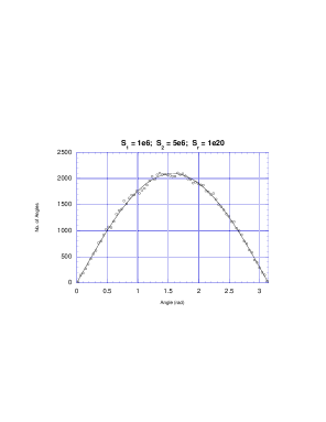
Figure 2. The distribution of angles versus angle: The dots represent the distribution of spectral points of the angle operator within a small angle $\delta\theta$. The solid curve is a plot of $\sin\theta$. The required spins are $10^{20}$ for geometric support and $10^{6}$ for the surface fluxes. (From Ref. [9])

The angle spectrum must also match the behavior of angles in three-dimensional space. In the classical, smooth model of angles the distribution of solid angles is proportional to $\sin\theta$. We expect that the discrete model of space should be able to reproduce this behavior in the appropriate limit. Therefore, the classical limit not only encompasses the need to achieve small angles and fine angular resolution, but also the need to match the distribution of solid angles [9]. In the discrete model this reduces to finding the number of intertwiners with a given core. This distribution can be found numerically. The results are shown in Fig. (2) for a choice of surface fluxes. Details of this calculation are in Ref. [9].

Though it is not obvious by looking at this one plot, to match the expected distribution of solid angle it is necessary that the geometric support $n_{r}$ be many orders of magnitude larger than the surface fluxes through $S_{1}$ and $S_{2}$. Further, the spin flux through the two surfaces must be approximately the same magnitude.

3. Quasilocal Energy

On spatial manifolds without boundary, the action for the classical (3+1) form of gravity is a set of constraints. Suppose that the space does have a boundary $\partial\Sigma$. Under the boundary conditions

$$\begin{split}&\delta E^{ai}|_{\partial\Sigma}=0\text{ which includes fixing the ``area density'' }n_{a}\delta E^{ai}|_{\partial\Sigma}=0\\ &N^{a}|_{\partial\Sigma}=0;\;\delta N|_{\partial\Sigma}=0\end{split}$$ (3)

the theory is inconsistent without the boundary term

$$H_{\partial\Sigma}(N)=\int_{\partial\Sigma}d^{2}x\epsilon^{ijk}Nn_{a}A_{b}^{i}E^{bj}E^{ak}.$$ (4)

(See Ref. [10] or, for a more general setting, Ref. [11].) This is the Hamiltonian for the system. The quantization of this observable is carried out in Ref. [12]. The most general form of the operator is

$$\hat{H}_{\partial\Sigma}(N)=-(4\pi G)\sum_{v\in S\cap\mathsf{G}}\,\sum_{I,J\dashv v}N_{v}\chi_{I}\frac{\hat{J}_{J}\cdot\hat{J}_{I}}{\left(\sqrt{\hat{A}_{v}}\right)^{3}}.$$ (5)

The first sum is over all the intersections $v$ of the surface with the spin network. The second sum is over all the incident edges $I$ and $J$. $N_{v}$ is the lapse at the intersection $v$; $\chi_{I}$ is a sign factor for the edges $I$; and $\hat{A}$ is the area operator.

The spectrum is most easily stated for two types of intersections. Type (i) intersections are transversal while type (ii) include all other intersections. For higher valence vertices, the intertwiner core is labeled with edges $p,n$ and $z$ corresponding to incident edges $I$ with positive, negative and zero values of $\chi_{I}$. For the operator defined in Eq. (5), one has for type (i)

$$\begin{split}\hat{H}_{\partial\Sigma}(N)\mid s\rangle&=m\sum_{v\in S\cap{\mathsf{G}}}N_{v}\sqrt[4]{n_{v}(n_{v}+2)}\mid s\rangle.\\ \text{For type (ii):}\\ \hat{H}_{\partial\Sigma}(N)\mid s\rangle&=m\sum_{v\in S\cap{\mathsf{G}}}N_{v}\frac{p_{v}(p_{v}+2)+n_{v}(n_{v}+2)-z_{v}(z_{v}+2)}{\left[2p_{v}(p_{v}+2)+2n_{v}(n_{v}+2)-z_{v}(z_{v}+2)\right]^{\frac{3}{4}}}\mid s\rangle.\end{split}$$ (6)

The fundamental mass scale is defined as

$$m:=\sqrt{\frac{\hbar}{4\pi G}}.$$

This is essentially the same scale as $\ell$ of the geometric observables.

There are two remarks to make: For type (i) intersections $v$, the quasilocal energy operator has eigenvalue $\epsilon_{v}$, which is related to the area as $\epsilon_{v}=(m/\ell)\sqrt{a_{v}}$ in which $a_{v}$ is the eigenvalue of the area operator. The quasilocal energy is a sum of contributions from each intersection; the energy is a sum of independent, non-interacting particle-like excitations. This vastly simplifies the statistical mechanics based on this Hamiltonian [14].

4. Summary

There are two new operators for spin net gravity, angle and quasilocal energy. With length, area, and volume they provide a number of ways in which we are able to explore this discrete model of space. The angle operator is the first geometric operator that is purely combinatorial; it depends only on the spins of the vertex, not on the scale $\ell$. This also means that it is free of the quantization ambiguity associated with the Immirzi parameter [13]. Further, the quantization of this operator suggests that scalar products also have discrete spectra. Though this has largely escaped notice, this obviously has far reaching consequences in a variety of high and low energy physics.

In the case of the angle, we learn that the semi-classical limit is not merely determined by large spins, but by large spins on the internal edges of the intertwiner located at the vertex. To correctly model the distribution of angles we require not only that these spins be large ($\sim 10^{6}$) but also that the geometric support be many orders of magnitude larger ($\sim 10^{20}$).

Both operators share what appears to be a common feature with all operators in spin net gravity, the spectra are discrete. What is utterly remarkable is not just this - the discrete spectra of geometric quantities - but what this implies for all of space, whether it be curved or flat. If this model is correct, fundamental quantum geometry affects flat-space physics. We have only just begun to realize the consequences of such a dramatic shift in the foundations of spacetime geometry.

References

- [1] Carlo Rovelli, “Loop Quantum Gravity,” Living Reviews in Relativity at http://www.livingreviews.org/Articles/Volume1/1998-1rovelli.
- [2] C. Rovelli and L. Smolin, “Discreteness of area and volume in quantum gravity,” Nuc. Phys. B 442, 593-622 (1995), Erratum Nuc. Phys. B 456 (1995) 753.
- [3] C. Rovelli and L. Smolin, “Spin Networks and Quantum Gravity” Phys. Rev. D 52 (1995) 5743-5759.
- [4] Roger Penrose, “Angular momentum: An approach to combinatorial spacetime” in Quantum Theory and Beyond edited by T. Bastin (Cambridge University Press, Cambridge, 1971); “Combinatorial Quantum Theory and Quantized Directions” in Advances in Twistor Theory, Research Notes in Mathematics 37, edited by L. P. Hughston and R. S. Ward (Pitman, San Fransisco, 1979) pp. 301-307; in Combinatorial Mathematics and its Application edited by D. J. A. Welsh (Academic Press, London, 1971); “Theory of Quantized Directions,” unpublished notes.
- [5] J. Baez, “Spin networks in gauge theory,” Advances in Mathematics 117 (1996) 253 - 272.
- [6] S. Major, “Operators for quantized directions” Class. Quant. Grav. 16 (1999) 3859; Online Archive: gr-qc/9905019.
- [7] N. Grot and C. Rovelli, “Moduli-space structure of knots with intersections” J. Math. Phys. 37 (1996) 3014-3021.
- [8] N. Grot, “Topics in Loop Quantum Gravity” MS Thesis University of Pittsburgh 1998.
- [9] M. Seifert, BA Thesis Swarthmore College in preparation.
- [10] V. Husain and S. Major, “Gravity and BF theory defined in bounded regions” Nuc. Phys. B 500 (1997) 381-401; Online Archive: gr-qc/9703043.
- [11] S. A. Major, “q-Quantum Gravity”, Ph.D. Dissertation, The Pennsylvania State University (1997).
- [12] S. A. Major, “Quasilocal energy for spin net gravity” Class. Quant. Grav. 17 (2000) 1467-1487; Online Archive: gr-qc/9906052.
- [13] G. Immirzi, “Quantum Gravity and Regge Calculus” Nuc. Phys. Proc. Suppl. 57 (1997) 65-72.
- [14] S. Major and K. Setter, “Gravitational Statistical Mechanics: A model” in preparation.