Gravitational Statistical Mechanics: A model

Abstract.

Using the quantum Hamiltonian for a gravitational system with boundary, we find the partition function and derive the resulting thermodynamics. The Hamiltonian is the boundary term required by functional differentiability of the action for Lorentzian general relativity. In this model, states of quantum geometry are represented by spin networks. We show that the statistical mechanics of the model reduces to that of a simple non-interacting gas of particles with spin. Using both canonical and grand canonical descriptions, we investigate two temperature regimes determined by the fundamental constant in the theory, $m$. In the high temperature limit ($kT\gg m$), the model is thermodynamically stable. For low temperatures ($kT\ll m$) and for macroscopic areas of the bounding surface, the entropy is proportional to area (with logarithmic correction), providing a simple derivation of the Bekenstein-Hawking result. By comparing our results to known semiclassical relations we are able to fix the fundamental scale $m$. Also in the low temperature, macroscopic limit, the quantum geometry on the boundary forms a ‘condensate’ in the lowest energy level ($j=1/2$).

1. Introduction

The statistical mechanics of the gravitational field will provide answers to some of the most intriguing questions on the relation between quantum and gravitational physics. These questions center on key issues such as the dominance of the semiclassical states, the states of geometry on the smallest possible scales (including microstates of black holes), the final stages of stellar collapse, and the early dynamics of the universe. While general gravitational statistical mechanics remains relatively unexplored, considerable progress has been made in understanding quantum black holes.

In the context of string theory, many properties of extremal and near extremal black holes have been derived. (See Ref. [1] for a review.) Within the context of four dimensional quantum gravity there has also been some progress. These have included studies of canonical ensembles for vacuum spacetimes in which one fixes the average mass of the system and computes thermodynamic quantities using the partition function. For Schwarzschild black holes, such canonical ensembles were considered in, for instance, Kastrup [2] and Mäkelä and Repo (who also consider the statistical mechanics of the exterior region) [3]. The partition function in both these cases is divergent. In statistical mechanics, one can introduce a chemical potential to tame the divergence of the canonical ensemble. This was done by Gour for black holes with area spectra given by integer multiples of a fundamental area [4].

The present work makes use of canonical quantum gravity using real connection variables [5], or, succinctly, “spin net gravity.” Spin networks, discovered in this context by Rovelli and Smolin [6], are linear combinations of Wilson loops based on Ashtekar’s new variables [7]. Spin networks are one of the central elements of this approach to the quantization of gravity. There is a primer on spin networks in Ref. [8] and a review of the general approach in Ref. [9]. The mathematics has evolved considerably and now provides rigorous underpinnings for the quantization [10] - [18] of the kinematic states of quantum gravity.

Perhaps the most striking result of this field is the new picture it provides of geometry on the fundamental scale. In this picture, 3-geometry is represented by a graph. A state of quantum geometry is built from holonomies of the gravitational connection along a collection of edges. These edges are “field lines of area” quite similar to electric field lines in electrostatics. This new “quantum geometry” is vastly different from our garden-variety geometry of meter sticks, particle accelerators, and regions neighboring black holes. Length [19], area ([6, 20, 21]), volume ([6, 22, 23, 24, 25]), and angle [26] have been found to have discrete spectra. In this approach to quantum gravity, geometry is fundamentally discrete.

Within the framework of spin net gravity, there have been a number of entropy calculations ([27] -[30]) which are largely based on the “area ensemble”. The idea is that one uses the area, instead of energy, as the fixed macroscopic parameter. The resulting ensemble is defined with respect to the area and its conjugate intensive quantity, the “area temperature” or surface pressure.

We take a different approach. Gravitational systems defined in bounded spatial regions generically have Hamiltonians associated with their boundaries. We formulate gravitational statistical mechanics using the quantum Hamiltonian and the usual partition function: a sum over all states of the Boltzmann weighting factor $e^{-\beta\hat{H}}$. This is only possible when the spatial manifold has boundary. In this case, the Hamiltonian is the quasilocal energy associated with the boundary. While our statistical mechanical treatment is familiar, the statistical sum is in stark contrast to familiar textbook presentations of statistical mechanics, where quantized matter fields are compared to classical geometry via the infinite volume limit. The ensembles we describe contain no matter nor is there a background geometry to compare to; this is the statistical mechanics of fundamental geometry.

Even without background geometry, we nevertheless can investigate three, separate limits to the theory: high and low temperatures and the macroscopic limit. The temperature regimes are determined by the scale of the theory, which is roughly the Planck scale. To investigate spatial boundaries with macroscopic areas, it is necessary to study the model when there are a very large number of intersections between the boundary and the underlying spin network graph. Combining both this macroscopic limit and the low temperature regime, we find that the entropy is proportional to area (with logarithmic correction) and that the system condenses in the lowest energy level.

These results come from a confluence of a number of features of this model. First, we make use of a quantum Hamiltonian of the system [31]. It has a very simple action on spin network states. Second, spin net gravity effectively reduces the study of quantum gravitational field theory to quantum gravitational mechanics. Our model is equivalent to a system of geometric particles. Third, there are clearly defined scales in which the theory must match previous results. This enables us to fix the fundamental scale of the theory.

In the next section, we define the model that forms the basis for our study. We give some of the necessary classical theory before reviewing the quantum theory and spin network states. At each stage we give the context to the assumptions behind the model. These assumptions are also collected in the final subsection (2.3). In Section 3, we study the canonical ensemble in the hot flat space limit and define the grand canonical ensemble in Section 4. This allows the study of the model in low temperature and macroscopic limits. Finally, the work is summarized and some implications are discussed in Section 5.

2. Defining the Model

We begin the study of general gravitational statistical mechanics with a simple model. To motivate the assumptions and to provide the necessary background, we discuss the classical theory, including boundary conditions, the quantum environment, the quantization of the Hamiltonian, and the scale of the theory. A summary of the model is given in 2.3.

2.1. Classical Hamiltonian Theory

We consider 4-dimensional spacetimes of the form $M=\Sigma\times{\mathbb{R}}$, where the spatial region $\Sigma$ has boundary. While there may be more than one component of the boundary in general, such as inner and asymptotic components, we focus entirely on a single, 2-sphere interior boundary, $\partial\Sigma$. We do not specify whether this is an intersection of the space with a horizon.

In the Hamiltonian formalism the classical fields on the phase space of general relativity can be expressed using connection variables [7, 5]. These connections are the configuration variables. The real, $su(2)$-valued connection is $A_{a}^{i}(x)$ where $a$ is a spatial index and $i$ is the index associated to the internal $su(2)$ space. The conjugate momenta, or “electric field” $E^{ai}(x)$, is a geometric variable related to the inverse spatial metric $q^{ab}$ by $E^{ai}E^{bi}=|q_{ab}|q^{ab}$. The determinant of the spatial metric is denoted $|q_{ab}|$. The kinematic phase space of quantum gravity is similar to SU(2) Yang-Mills theory. The key difference is the absence of background geometry.

Set in a spatially bounded region, classical Hamiltonian gravity provides a clear selection criteria for the quasilocal energy: The ($3+1$)-action must be functionally differentiable. This ensures that histories remain within the phase space. In general, the method of functional differentiability generates boundary conditions on the phase space variables, gauge parameters, and surface terms [32, 33]. Depending on the nature of the boundary conditions, surface terms may be added to the action to make the theory well-defined. These surface terms, without which the theory would be inconsistent, are the fundamental observables.

The Hamiltonian of the theory is the surface observable arising from Hamiltonian constraint and is enforced by the lapse function ${\cal N}$. This surface observable is the quasilocal energy and reduces to the ADM energy in asymptopia [32]. It is also the surface term which satisfies the correct algebra: The surface term generated by the Hamiltonian constraint satisfies the same algebra as the constraint itself [32, 33]. For these reasons, we use the surface term arising from the Hamiltonian constraint as the definition of the quasilocal energy and call it the Hamiltonian.

In the real connection variables, the variation of the connection in the Hamiltonian constraint generates a surface term which must either vanish when boundary conditions are applied or be canceled by the surface term

$$H_{\partial\Sigma}({\cal N})=\frac{1}{4\pi G}\int_{\partial\Sigma}d^{2}x\epsilon^{ijk}{\cal N}n_{a}A_{b}^{i}E^{bj}E^{ak}.$$ (1)

The lapse ${\cal N}$ has a density weight of $-1$. When the lapse is non-vanishing on $\partial\Sigma$, the surface term of Eq. (1) must be added to the Hamiltonian constraint. This classical expression reduces to the quasilocal energy of Brown and York [34], to the ADM energy in asymptopia, and to the Misner-Sharp mass in spherical symmetry [32]. This Hamiltonian is the surface term which ensures functional differentiability of Lorentzian general relativity in terms of real connection variables.

With the addition of the Hamiltonian of Eq. (1) the boundary conditions required by functional differentiability of the Hamiltonian constraint are simply expressed. Let $\kappa^{abi}={\cal N}\epsilon^{ijk}E^{aj}E^{bk}$, then $\delta n_{a}\kappa^{abi}|_{\partial\Sigma}=0$. However, a complete set of boundary conditions includes kinematic boundary conditions, which arise from functional differentiability of the Gauss, diffeomorphism, and Hamiltonian constraints, and dynamic boundary conditions. Dynamic boundary conditions ensure that the boundary conditions are preserved under evolution. These are found by computing the constraint algebra. See Ref. [32] (or, for a more general analysis, Ref. [33]) for details.

One set of kinematic boundary conditions which ensures functional differentiability of the constraints with the surface term of Eq. (1) is

$$\begin{split}&\delta(n_{a}\epsilon^{ijk}E^{aj}E^{bk})|_{\partial\Sigma}=0\\ &\delta{\cal N}|_{\partial\Sigma}=0\text{, the lapse is fixed, and}\\ &N^{a}|_{\partial\Sigma}=0\text{, so that spatial diffeomorphisms vanish on the boundary.}\end{split}$$ (2)

To ensure that the theory is dynamically well-defined one must impose further boundary conditions on $\partial\Sigma$. One consistent set is

$$\begin{split}&D_{b}\kappa^{abi}|_{\partial\Sigma}=0\\ &\Lambda^{i}|_{\partial\Sigma}=0\\ &\partial_{a}{\cal N}|_{\partial\Sigma}=0\text{ so that the lapse is fixed to be a constant on }\partial\Sigma.\end{split}$$ (3)

We choose the constant lapse to be 1.

Both sets of boundary conditions, Eqs. (LABEL:kbcs) and (LABEL:dbcs), comprise a complete, consistent set of boundary conditions for the model. As is clear from these conditions, the model is defined for hypersurface orthogonal spatial boundaries with fixed electric field. Finally, we note that these boundary conditions are not in the category of boundary conditions which includes isolated horizons. Isolated horizons require that the lapse vanish on the horizon [30].

2.2. Quantum Domain

To investigate quantum statistical mechanics, one must investigate both the Hilbert space of the bounded theory and the action of the quantum Hamiltonian. We give an outline of the state space framework here though the reader is encouraged to refer to references [10, 11, 12, 13, 14, 15, 16, 17, 18] for the elegant theory behind this sketch. The quantum degrees of freedom are captured by holonomies along paths embedded in $\Sigma$. Gravitational analogs of Wilson loops, a holonomy of the connection gives an element of SU(2). This simple observation is the key to the quantum configuration space. One defines a generalized connection to be a map from each path to the group. Like the holonomy of the classical connection, the generalized connection describes parallel transport along paths. It is convenient to describe a collection of paths by a set of edges of a single graph. With the definition of generalized connections and a graph, one can introduce a measure on the space of generalized connections simply by using the $SU(2)$ Haar measure on every edge. It turns out that the space of generalized connections is the completion of the space of smooth connections [10, 11]. This space is the quantum configuration space. A basis on this space is described by spin networks [12].

An open spin network $s$ consists of the triple $({\sf G},{\bf n,i})$. The graph ${\sf G}$ is embedded in the 3-dimensional space and is comprised of a set of edges and vertices. Each edge is assigned a nontrivial, irreducible representation of $SU(2)$. On every edge $e$ this representation is labeled by an integer $n_{e}$ from the set ${\bf n}$ where $n=2j$. The minimum representation, or edge label, is $n=1$. The edges intersect at vertices. The number of edges incident to a vertex is called the valence. In this model valence-one vertices, the “open edges,” only occur at the intersection of the graph with the boundary. Intertwiners, ${\bf i}$, assign to each vertex $v$ a vector $i_{v}$ in the tensor product of the representations labeling the edges incident to the vertex $v$. If a vertex is in the interior, the vector $i_{v}$ is invariant under the action of $SU(2)$. If the vertex lies on the boundary, $i_{v}$ is not invariant under $SU(2)$. We label these boundary intertwiner vectors by an integer which corresponds to the $m_{j}$ values familiar from angular momentum.

In more picturesque language, edge labels record the number of spin-$1/2$ “threads” in a single edge of a spin network. Intertwiners label the ways in which all incident threads are connected. Vertices at the ends of the open edges are labeled by the state of the spin-$1/2$ threads.

Notice that any open spin network determines a set of valence-one vertices, which determine a Hilbert space given by a product of angular momentum states $\mid j\,m_{j}\rangle$. These are the states on the boundary of the space that determine the quasilocal energy.

We base the statistical mechanics on the quantization of the boundary Hamiltonian of Eq. (1). Using loop techniques and recoupling theory, the boundary Hamiltonian of Eq. (1) can be quantized [31]. The quantization of the Hamiltonian is not free of choices. However, the most general form of the operator is, for transversal edges,

$$\hat{H}_{\partial\Sigma}\mid s\rangle=m\sum_{v\in\partial\Sigma\cap{\sf G}}{\cal N}_{v}\sqrt[4]{n_{v}(n_{v}+2)}\mid s\rangle.$$ (4)

This operator depends only on vertices in the boundary. The lapse ${\cal N}_{v}$ is the scalar (vanishing density weight) lapse at the vertex $v$. In light of the boundary conditions of Eq. (LABEL:dbcs), the lapse is constant on the boundary. We set ${\cal N}_{v}=1$ for all boundary vertices $v$.

There are two properties of the Hamiltonian operator of Eq. (4) which impact the statistical mechanics. First, each edge contributes to the energy independently of the other edges. This simplifies the model considerably, as the total quasilocal energy is the sum of the contributions of each edge. Thus, as we will see, the problem reduces to a gas of nearly identical particles. Second, as is clear from the form of the Hamiltonian operator of Eq. (4), the energy of the system does not depend on the vectors of the boundary vertices; the $m_{j}$ value does not count. Thus, the system is degenerate.

There is an important caveat to this degeneracy. We define the model only through the component of the system which determines the energy, the boundary theory. If one were to include considerations of the interior state, one would include the vast degeneracy, presumably infinite, of the interior intertwiner bases, knot states of the edges, and other diffeomorphism invariant aspects of the spin network graph [35].

In statistical mechanics, the macroscopic behavior depends critically on the particle statistics. In our model the intersections of the surface with the network define a set of independent, distinguishable particles with spin. We take particles with different spin to be distinguishable. To motivate this it is best to describe measurements on the fundamental geometry.

In quantum geometry, each intersecting edge determines the ‘local’ shape of the surface. Not only does a label $n$ determine the area contribution of a single edge, but the vertex also can determine the local curvature, as in Ref. [30]. As observed from the interior, the labels on these edges - the amount of geometric flux - are measurable via the area operator. Fluctuations in these labels are, in principle, observed as localized sources of radiation. The expectation is that, even if the macroscopic geometry is symmetric, the quantum geometry will be fluctuating on the microscopic scale. The localization can be achieved with the spin network itself if the spin network is sufficiently complex. Thus, simply based on the abstract graph, its labels and its intertwiners, we expect that it is possible to distinguish spin network edges and their fluctuations. This result may also be derived by examining the role of diffeomorphisms on the boundary [27].

With these considerations the following picture emerges: Gravitational statistical mechanics of the model is based on a set of non-interacting particles. Two geometric particles are distinguishable if they have different spins. The particles induced from an edge with label $n$ have a degeneracy of $n+1$.

2.3. Scale, Parameters, and Summary

The constant $m$ in Eq. (4) sets the fundamental scale of the theory. It is the same scale as that of the length $\ell$ which appears in the geometric observables. For instance, the area contribution of a single edge $e$ is given by $\ell^{2}\sqrt{n_{e}(n_{e}+2)}$. The two parameters $m$ and $\ell$ are inversely related with $m=\hbar/\ell$.

We retain the overall scale parameter in terms of $m$ or $\ell$. There are two reasons for doing this. First, we wish to derive the relation between the fundamental scale of the model and the Planck length $l_{P}:=\sqrt{\hbar G/c^{3}}$. Second, this enables us to address a subtlety arising in the definition of the connection. As Immirzi has emphasized, in the canonical transformation used to define the connection variables there is a family of choices generated by one non-zero, real parameter $\gamma$, ${}^{\gamma}A_{a}^{i}=\Gamma_{a}^{i}-\gamma K_{a}^{i},{}^{\gamma}E^{ai}=(1/\gamma)E^{ai}$ [36]. We absorb $\gamma$ into the constants $m$ and $\ell$. Finally, we retain Boltzmann’s constant $k$ throughout.

Since $m$ sets the scale, the regimes of interest are determined relative to this constant. The significant dimensionless parameter is the ratio of this energy scale to the thermal energy, $\beta m$. Temperatures of order unity ($T\sim 1/km$) are roughly $10^{32}$ K, so garden-variety energy scales of the universe are far below the natural scale of the theory; for quantum geometry, the universe is a chilly place. Thus the more realistic regime is the low temperature limit. Throughout this paper we also use such terms as “microscopic” and “macroscopic.” By microscopic we mean boundaries with area on the order of $\ell^{2}$. By macroscopic we mean boundaries with areas much greater than $\ell^{2}$, i.e. boundaries on scales of elementary particles up through astrophysical objects. As we see in Section 4, to use microscopic results in the macroscopic regime requires a study of the scaling of physical quantities as they diverge. All semiclassical results need to be closely examined in low temperature, macroscopic limits.

When we compare the thermodynamics of this model with semiclassical results, we fix the fundamental scale of the theory. This is done in Section 4.2, where we compare the area-entropy relationship of our model to the Bekenstein-Hawking area-entropy relation.

In summary, the remainder of the paper deals exclusively with the model defined by:

1. A spatial manifold having boundary $\partial\Sigma$.

2. We assume that the quantum boundary conditions are a straightforward implementation of the classical boundary conditions of Eqs. LABEL:kbcs and LABEL:dbcs.

3. A quantum Hamiltonian given by Eq. (4) with:

   1. Fixed, unit lapse on $\partial\Sigma$,

   2. A degeneracy of $n_{e}+1$ associated to every edge $e$.

4. We assume valence-one boundary vertices, i.e. the intersections ${\sf G}\cap\partial\Sigma$ occur along single edges

5. We assume edges with different spins can be distinguished.

Hence, the model reduces to a non-interacting, degenerate gas of distinguishable particles with spin.

3. Canonical ensemble

This section provides groundwork for both the canonical and grand canonical ensembles. In the canonical ensemble, we concentrate on the high temperature limits of the theory.

Given any boundary with non-vanishing area, a set of edges will intersect the boundary. In the canonical ensemble, we fix the total number of intersections between the spin network graph and the boundary $\partial\Sigma$ to be $N$, while allowing the energy of the system (the labels on the edges) to fluctuate. These intersecting edges are the only edges in the spin network that are open.

We investigate the statistical mechanics of $N$ distinguishable non-interacting geometric particles. To specify a state of the system, we need two things: a list of edge labels $\{n_{i}\}$ for those edges that intersect the boundary $\partial\Sigma$, and an “$m_{j}$” value for each of these edges. Since the particles are distinguishable, $\{n_{i}\}$ will be an ordered list.

The canonical partition function, $Z=\text{Tr }e^{-\beta\hat{H}}$, becomes

$$Z_{N}(T)=\sum_{\{n_{i}\}}g(\{n_{i}\})\>e^{-\beta(\epsilon_{n_{1}}+\dots+\epsilon_{n_{N}})}$$ (5)

with the quantum Hamiltonian of Eq. (4) with unit lapse. The energy contribution of the $i$th edge is given by $\epsilon_{n_{i}}:=m\sqrt[4]{n_{i}(n_{i}+2)}$, where $m$ is the fundamental mass scale for the system. The degeneracy due to the boundary vertices is

$$g(\{n_{i}\})=\prod_{i=1}^{N}(n_{i}+1).$$ (6)

As the particles are independent, the partition function reduces to

$$Z=\left(\sum_{n=1}^{\infty}(n+1)e^{-\beta\epsilon_{n}}\right)^{N}.$$ (7)

With this partition function it is an easy matter to compute the thermodynamic potential

$${\cal A}=-\frac{1}{\beta}\ln Z=-\frac{N}{\beta}\ln f,$$ (8)

where

$$f:=\sum_{n=1}^{\infty}(n+1)e^{-\beta\epsilon_{n}}$$ (9)

is the one particle partition function.

Normally at this stage one would study the behavior of the partition function and thermodynamic quantities in the infinite volume limit. As we are studying the underlying geometry itself, we cannot do this. We have no background for comparison. Nonetheless, we can explore the high temperature limit.

In the high temperature limit, $\beta m\ll 1$, the sum in $f$ may be approximated by an integral which can be integrated exactly

$$\begin{split}f&\approx\int_{1}^{\infty}(n+1)e^{-\beta\epsilon_{n}}\\ &=\frac{2}{(\beta m)^{4}}\,e^{-\sqrt[4]{3}\beta m}\left(6+6\sqrt[4]{3}\beta m+3\sqrt{3}(\beta m)^{2}+\sqrt[4]{3^{3}}(\beta m)^{3}\right).\end{split}$$ (10)

The single particle partition function behaves as

$$f\approx\frac{12}{(\beta m)^{4}}-\frac{3}{2}+O(\beta m)\approx\frac{12}{(\beta m)^{4}}$$ (11)

for high temperatures. In this temperature regime, physical quantities are easy to compute. The entropy is

$$S=-\frac{\partial{\cal A}}{\partial T}=kN\left(\ln 12-4\ln(\beta m)+4\right).$$ (12)

The heat capacity simply scales with the number of intersections

$$C=T\frac{\partial S}{\partial T}=4kN.$$ (13)

As $C>0$, Le Châtelier’s principle is satisfied and the system is thermally stable. One initially would expect that since the behavior of Hawking radiation requires that the specific heat of black holes to be negative, this high temperature result would preclude black holes. However, there are quite general arguments [37] that the specific heat of Lorentzian black holes ought to be positive. Further, York [38] found that, using Hawking’s result for spherically symmetric black holes, black holes in a box can be thermodynamically stable. In fact, York found that there were two possible mass solutions, with one stable and one unstable. He described these as two different phases of the system, one with stable black holes and one of hot flat space. To map out the correspondence between the model York considers and the present model, we would need to add an additional boundary and a parameter which measured the size of the outer boundary. The topology of our present model prevents us from seeing both solutions.

Average energy and area are also easy to compute. The average energy is given by

$$\langle E\rangle:=\sum_{i=1}^{N}\langle E_{i}\rangle$$

with

$$\langle E_{j}\rangle=\frac{1}{f}\sum_{n_{j}=1}^{\infty}\epsilon_{n}e^{-\beta\epsilon_{n}}.$$

Since all the expectation values for each of the particles are all identical, $\langle E\rangle=N\langle E_{i}\rangle$ for any $i$. In the high temperature regime we make the approximation

$$\langle E_{i}\rangle\approx\frac{m}{f}\int_{1}^{\infty}dx(x+1)\sqrt[4]{x(x+2)}e^{-\beta m\sqrt[4]{x(x+2)}}.$$

The integral can be done exactly. The leading order behavior gives a total average energy of

$$\langle E\rangle=4NkT$$ (14)

in the high temperature limit. Similarly, the area of the bounding 2-surface, in the high temperature limit, is given by

$$\langle A\rangle=20\ell^{2}N\left(\frac{kT}{m}\right)^{2}.$$ (15)

All of these physical quantities are proportional to the number of intersections $N$. From the entropy (12) and the area (15) results, we see that the entropy and area obey the Bekenstein-Hawking proportionality $S=k\tfrac{A}{4\ell^{2}}$ only at specific temperatures. In this high temperature approximation, this occurs when $\beta m\approx 0.78$ and $5.8$. Since the Bekenstein-Hawking result is valid in lower temperatures ($\beta m\gg 1$), these are spurious solutions.

It is perhaps not surprising that semi-classical physics differs with these results at high temperature scales. We should not be surprised to discover that the semi-classical calculations, derived in the low temperature domain, do not agree with results derived for temperatures much greater than the Planck scale!

As is often the case in statistical mechanics, to investigate lower temperatures it proves easier to work with the grand canonical ensemble. This is what we turn to next.

4. Grand Canonical Ensemble

In the statistical mechanics of particles the grand canonical ensemble includes varying particle number. In this case we allow the number of intersections between the spin network state and the boundary to fluctuate. This means that we consider the category of dynamics in which spin network states evolve by changing the underlying graph in a manner consistent with kinematical constraints and boundary conditions.

A new element in our approach is the use of the chemical potential. Though used in the Schwarzschild case in Ref. [4], the chemical potential has not been used within the context of spin net gravity. Allowing the number of particles to fluctuate provides a number of benefits. The scale of the theory, $m$, is so large that, in the canonical ensemble, any change of the system is fantastically unlikely for temperatures such as occur in our universe. The dynamics appears to be “frozen”. Indeed, the analysis would seem to require that all geometric objects have only two spin-$1/2$ edges! The chemical potential allows interesting behavior to occur at lower temperatures and for macroscopic configurations. Further, the chemical potential provides a measure of the geometric interaction between the interior and the boundary.

Calling the number of intersections, $N$, and the chemical potential, $\mu$, the resulting grand canonical partition function is

$${\cal Z}(T,\mu)=\sum_{N=1}^{\infty}\sum_{\{n_{i}\}}g(\{n_{i}\})e^{-\beta\left(\epsilon_{n_{1}}+\dots+\epsilon_{n_{N}}-\mu N\right)},$$ (16)

where, as before, $g(\{n_{i}\})$ is the degeneracy of the edge states. Since we consider boundaries with non-vanishing area, the sum over $N$ begins at $1$. Each edge independently contributes to energy, so the partition function simplifies.

$${\cal Z} = \sum_{N=1}^{\infty}\left(\sum_{n=1}^{\infty}(n+1)e^{-\beta(\epsilon_{n}-\mu})\right)^{N}$$

$$= \frac{fz}{1-fz}$$

in which the fugacity $z$ is defined as usual, $z=e^{\beta\mu}$, and $f$ is defined in Eq. (9).

This partition function diverges as $fz$ approaches 1. There is physics in this divergence. To investigate the divergence we first compute some physical quantities.

The thermodynamic potential is given by

$$\Omega=-kT(\ln fz-\ln(1-fz)).$$ (18)

The ensemble average of the number of intersections is

$$\langle N\rangle=-\frac{\partial\Omega}{\partial\mu}=\frac{1}{1-fz}.$$ (19)

For physical configurations, the ensemble average $\langle N\rangle$ must be greater than or equal to 1. The lower bound, $\langle N\rangle=1$, introduces a relation between temperature and chemical potential,

$$\mu=-\frac{\ln f}{\beta},$$

which selects physical configurations when the boundary has non-vanishing area. A plot of the relation $\langle N\rangle=1$ is given in Fig. (1).

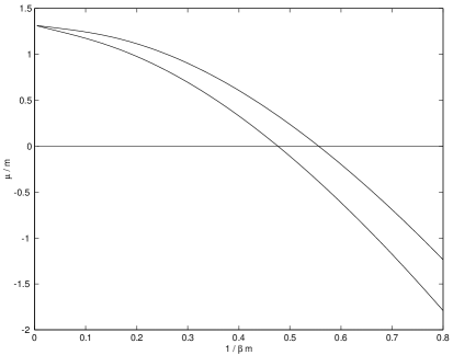
Figure 1. The restriction that the average number of intersections be greater or equal to 1, $\langle N\rangle\geq 1$, yields a relation between the temperature and the chemical potential. The upper curve is the plot of the relation, $\langle N\rangle=1$. There is a maximum temperature for every chemical potential. The lower curve, or “macroscopic curve,” is the relation $fz=1$ which corresponds to infinite intersection number. The curve near zero temperature is roughly linear, with a slope of about $-0.7$ and an intercept of $\sim\sqrt[4]{3}$. Both curves have an error on the order of $10^{-3}$ at the Planck temperature $\beta m=1$.

The number of intersections diverges when the product $fz$ approaches 1. Since $f$ is a monotonically increasing function of the temperature, these restrictions yield a maximum temperature for every chemical potential. This relation is the upper curve in Fig. (1). Temperatures higher than shown in the figure send the partition function to infinity and $\langle N\rangle$ to unphysical, negative values. All physical configurations lie inside the region between the two curves in Fig. (1). We call this region bounded by the curves $\langle N\rangle=1$ and $fz\simeq 1$ the “macroscopic band.”

To better understand the geometry at the divergence, when $fz\rightarrow 1$, it is worth deriving the area of the bounding surface. The area may be obtained through the simple relation between the Hamiltonian and the area at each intersection $i$ [31]

$$\frac{\epsilon_{i}}{m}=\frac{\sqrt{a_{i}}}{\ell^{2}}.$$ (20)

A short calculation shows that

$$\langle A\rangle=\frac{1}{{\cal Z}}\sum_{N=1}^{\infty}N(fz)^{N}\frac{1}{f}\sum_{n=1}^{\infty}a_{n}(n+1)e^{-\frac{\beta m}{\ell}\sqrt{a_{n}}}.$$

Thus,

$$\langle A\rangle=\langle N\rangle\langle a\rangle,$$ (21)

in which $\langle a\rangle$ is the single particle average area.

Since the area scales with $\langle N\rangle$, macroscopic areas occur for large $\langle N\rangle$. The divergence $\langle N\rangle\rightarrow\infty$ when $fz\rightarrow 1$ is physical in that the divergence selects the region of parameter space where macroscopic objects live. In this model of discrete space, macroscopic objects are found in $(1/\beta m,\mu/m)$ space between the curves shown in Fig. (1).

At low temperatures, it is easy to characterize the macroscopic limit. When $\beta m\gg 1$, $fz$ may be expressed as

$$fz=2e^{-\beta(\epsilon_{1}-\mu)}\left(1+\sum_{n=2}^{\infty}\left(\frac{n+1}{2}\right)e^{-\beta(\epsilon_{n}-\epsilon_{1})}\right)=2e^{-\beta(\epsilon_{1}-\mu)}+O(e^{-\beta m\Delta}),$$ (22)

where $\Delta:=(\sqrt[4]{8}-\sqrt[4]{3})$ is the numerical difference in the first two energy levels. Neglecting the higher order terms, the macroscopic condition $fz\simeq 1$ gives us

$$\mu\simeq-\frac{\ln 2}{\beta}+\epsilon_{1}.$$ (23)

This relation, the low temperature, leading order approximation to the top curve in Fig. (1), proves useful when comparing the entropy and area. We continue to use the “$\simeq$” whenever we express quantities in the low temperature, macroscopic limit.

4.1. Condensation

By examining the occupation numbers of the edge labels, one can find macroscopic occupation of the lowest level. If one rewrites the partition function in terms of number of intersections at the $k$th level, $N_{k}$, then one quickly finds the average

$$\langle N_{k}\rangle=-\frac{1}{\beta}\frac{\partial\ln{\cal Z}}{\partial\epsilon_{k}}=\frac{(k+1)e^{-\beta\epsilon_{k}}}{f(1-fz)}.$$

As might be expected, these quantities diverge with $\langle N\rangle$ for all $k$. It is more interesting to investigate how the relative proportions $\langle N_{k}\rangle/{\langle N\rangle}$ behave. The ratio is

$$\frac{\langle N_{k}\rangle}{\langle N\rangle}=\frac{k+1}{f}e^{-\beta\epsilon_{k}}$$ (24)

which, curiously, is independent of the fugacity $z$. With the same techniques just employed in the limit for $fz$ in Eq. (22), at low temperatures the occupation of the lowest possible level, $k=1$ behaves as

$$\frac{\langle N_{1}\rangle}{\langle N\rangle}\simeq 1-O(e^{-\beta m\Delta}).$$ (25)

As $\langle N\rangle$ becomes macroscopic, so does $\langle N_{1}\rangle$. The system “condenses” in the spin-$1/2$ state, meaning that in the limit of large $\langle N\rangle$ and at low temperatures, the occupation of the lowest state accounts for virtually all the particles. This is much like Bose-Einstein condensation, which is characterized by a finite fraction of states in the zero momentum state in the infinite particle limit

$$\lim_{N\rightarrow\infty}\frac{\langle n_{0}\rangle}{N}>0.$$

If the ratio vanishes in the limit, then there is no condensation. While the analogous ratio in the quantum gravity case, Eq. (25), is positive and near unity, it is difficult to be precise as the $\langle N\rangle\rightarrow\infty$ condition is the macroscopic limit and results in a more complicated relation between $\mu$ and $\beta$. (The condition $fz\simeq 1$ ties the chemical potential to the temperature, producing the macroscopic curve.) Nevertheless, it is easy to characterize the system in the low temperature limit; the model relaxes exponentially into the lowest state as the ratio of neighboring low lying states

$$\frac{\langle N_{2}\rangle}{\langle N_{1}\rangle}=\frac{3}{2}e^{-\beta m(\sqrt[4]{8}-\sqrt[4]{3})}$$

vanishes exponentially as $T\rightarrow 0$.

There is another difference between the condensation in this model and in a Bose-Einstein system. The fluctuations, $\langle\Delta N^{2}\rangle=\langle N^{2}\rangle-\langle N\rangle^{2}$, in intersection number behave as

$$\langle\Delta N^{2}\rangle=\frac{fz}{(1-fz)^{2}}.$$

Hence, the relative dispersion $\langle\Delta N^{2}\rangle/\langle N\rangle^{2}$ goes to 1 in the low temperature, macrcoscopic limit. The relative dispersion of the number of intersections at the lowest level also behaves this way. In a Bose-Einstein system, the analogous relative dispersions would vanish at low temperatures. In our model, despite the fact that the spin-$1/2$ state is macroscopically occupied, we still have a tempest of fluctuations. As discussed in Section 5 these fluctuations lead to potentially observable effects.

4.2. Gravitational thermodynamics

To check whether this model of quantum gravitational statistical mechanics reproduces the results of gravitational thermodynamics, we first derive the remaining macroscopic parameters of the system, entropy and average energy. Since we have not specified the boundary conditions so carefully as to pick out a black hole solution, it is interesting to see whether the relations of black hole mechanics are included in our thermodynamics. The remaining physical quantities are derived in a straightforward way, using standard statistical mechanics.

Defining the ensemble average of energy of a single intersection as

$$e:=\sum_{n=1}^{\infty}\epsilon_{n}(n+1)e^{-\beta\epsilon_{n}},$$

the energy is given by

$$\langle E\rangle=-\frac{\partial\ln{\cal Z}(T,z)}{\partial\beta}=\langle N\rangle\frac{e}{f}.$$ (26)

The entropy is given by

$$S=-\left(\frac{\partial\Omega}{\partial T}\right)_{\mu}=k\ln\langle N\rangle+k\ln(fz)+\frac{1}{T}\langle E\rangle-\frac{\mu}{T}\langle N\rangle.$$ (27)

The first thermodynamic relation we study is the Bekenstein-Hawking formula $S=kA/4l_{P}^{2}$. A quick glance at the equations for area, entropy, and energy in this model show a more complicated dependence than this simple proportionality. However, this is to be expected as the thermodynamic result holds at low temperatures and macroscopic geometries. At low temperatures, the area of Eq. (21) is simply $\langle N\rangle$ times the basic area element,

$$\langle A\rangle\simeq\ell^{2}\sqrt{3}\langle N\rangle,$$

so that the area scales with the number of intersections.

Using the relation between chemical potential and $\beta$ at low temperatures, Eq. (23), we find that

$$S\simeq k\frac{\ln 2}{\sqrt{3}}\frac{\langle A\rangle}{\ell^{2}}+k\ln\left(\frac{\langle A\rangle}{\ell^{2}}\right)$$ (28)

in the low temperature, macroscopic limit. This establishes the proportionality between entropy and area, with a logarithmic correction. This is identical to the result for black holes!

The reason for the proportionality factor $\ln 2/\sqrt{3}$ is easy to see. Suppose the surface area is quantized with uniformly spaced levels $A=n\alpha l^{2}$, where $n=1,2,\ldots$, $\alpha$ is a fixed parameter, and $l$ is the fundamental length. This suggests that the bounding surface is like a quilt sewn together of Planck scale patches, each of area $\alpha l^{2}$. If every patch has two possible states, then a surface of area $A=n\alpha l^{2}$ has $2^{n}$ surface states. This degeneracy contributes to the entropy and $S=\ln 2^{n}=\ln 2(A/\alpha l^{2})$. This is precisely what we have in Eq. (28), with $\alpha=\sqrt{3}$. Thus, the entropy is equal to the log of the number of states of the lowest level times the number of units of the fundamental area element $\sqrt{3}\ell^{2}$.

In the context of non-perturbative quantum gravity, a logarithmic correction has been derived before by Kaul and Majumdar [40]. However, they found that the correction term was negative, indicating that the semiclassical result was the maximal entropy. In other derivations of the logarithmic term, the corrections arise from quantum effects involving matter fields on a classical background.

To reproduce the thermodynamic result of Bekenstein, we fix the fundamental scale of the theory. We find that

$$\ell=\frac{1}{2}\sqrt{\frac{\sqrt{3}}{\ln 2}}l_{P}.$$ (29)

Matching with the thermodynamic result also fixes our fundamental energy scale.

It is also interesting to investigate the mass-temperature relation for spherical black holes to see whether these solutions also are found in this class of gravitational statistical mechanics models. The expected relation is given by

$$\langle M\rangle\propto\frac{1}{T}.$$

Since the energy is simply proportional to the intersection number and the temperature, it seems that this model appears not to include black hole solutions of this type.

While the results for spherically symmetric black holes do not match the thermodynamics of this ensemble, the entropy bound [41]

$$\frac{S}{k}\leq 2\pi RE$$ (30)

is satisfied with the areal radius definition $R:=\frac{1}{2}\sqrt{\frac{\langle A\rangle}{\pi}}$. To leading order in $\langle N\rangle$, the entropy $S$, energy $\langle E\rangle$ and area $\langle A\rangle$ scale with $\langle N\rangle$. Therefore we have from Eq. (30) that $\langle N\rangle\leq\langle N\rangle^{3/2}$, which is satisfied by all $\langle N\rangle$; this is not a tight bound! The result indicates that the ensembles we have considered do not contain black holes, which are conjectured to saturate this bound.

Further refinements of this model, including the implementation of admissibility conditions due to the topology of the boundary and gauge invariance, may be found in Ref. [39].

5. Discussion

In this work we have shown that a straightforward application of the ideas of statistical mechanics to a gravitational model yield results strikingly similar to black hole thermodynamics. In particular, using the grand canonical partition function we have shown that in the low temperature, macroscopic limit the system obeys the Bekenstein-Hawking entropy relation and the Bekenstein entropy bound. A new result is that the system condenses in the lowest level state in the low temperature, macroscopic limit.

Unlike the previous work in spin net quantum gravity, this work begins with the quantum gravitational statistical mechanics based on the Boltzmann weight $e^{-\beta\hat{H}}$. The pathbreaking work in Refs. [27, 28, 29, 30] based the statistical weight on the concept of the “area ensemble,” in which the Boltzmann weight is based on the extensive parameter area and its conjugate surface pressure. Here, we simply explore the statistical mechanics of the Lorentzian gravitational model defined in Section 2. It is a model in which the degrees of freedom of quantum geometry are encoded in non-interacting particles with spin. We do not specify black hole or isolated horizon boundary conditions and yet observe much the same thermodynamics.

There are several technical remarks which ought to be mentioned. We remind the reader that the quasilocal operator used in this paper is a candidate operator. In fact, in Ref. [31] there are two inequivalent expressions for the boundary Hamiltonian corresponding to two separate normalizations. In one, the operator is expressed in terms of the area operator (which provides the quantization of the $\sqrt{|q_{ab}|}$ in the lapse of Eq. (1)). This is the operator used in this paper. However, the spectrum of the quasilocal energy operator is modified when vertices lie on the bounding surface. The spectrum for higher valence vertices (type (ii)) is given by

$$\hat{E}_{\partial\Sigma}({\cal N})\mid s\rangle=m\sum_{v\in\partial\Sigma\cap{\mathsf{G}}}{\cal N}_{v}\frac{p_{v}(p_{v}+2)+n_{v}(n_{v}+2)-z_{v}(z_{v}+2)}{\left[2p_{v}(p_{v}+2)+2n_{v}(n_{v}+2)-z_{v}(z_{v}+2)\right]^{\frac{3}{4}}}\mid s\rangle.$$

This could be incorporated into the present context by adding another chemical potential. Simple statistical arguments suggest that in a fluctuating surface the dominant contribution would come from the bivalent intersections used here.

The second operator in Ref. [31] uses a distinct quantization of the classical Hamiltonian. The essential difference is that the determinant of the metric is incorporated using the volume operator. Both operators are well-defined but on different spaces. This operator requires that the intersections between the spin network state and the boundary are all valence one (type (i)), meaning that graphs on which states are based cannot have edges tangent to the surface $\partial\Sigma$. This spectrum of this operator is

$$\hat{E}_{\partial\Sigma}({\cal N\!\!\!\!\!_{{}_{\sim}}}\,)\mid s_{i}\rangle=m\sum_{v}{\cal N}_{v}\frac{n_{v}(n_{v}+1)}{\lambda_{v}}\mid s_{i}\rangle,$$ (31)

where $\lambda_{v}$ is the eigenvalue of the volume [6, 25]. On account of the state restriction, the numerator always has the simple form of the area operator; the operator is proportional to $\hat{A_{v}}^{2}/\hat{V_{v}}$. The eigenvalues $\lambda_{v}$ can be computed using recoupling theory [25]. However, since one can always find a surface tangent to a given edge of an embedded graph, the requirement of “no tangent edges” seems too strict to apply to general boundaries.

Throughout the statistical mechanic computation we set the lapse to 1 on the bounding surface $\partial\Sigma$. Since the lapse is fixed and constant by the boundary conditions, our choice is one solution. This choice, however, reflects the reparameterization freedom of time and the selection of which temperature we choose to use to investigate the model. Thus, the present statistical mechanics is for an observer at the spatial boundary with unit lapse. It would be interesting to investigate a model with another boundary and a parameter which measured its size so that one could compare solutions as in Ref. [38].

We close with three comments on the wider implications of this work. In the low temperature, macroscopic limit the boundary particles condense into the lowest level. Each spin network edge contributes roughly a Planck area ($\sqrt{3}\ell^{2}$) and has a degeneracy of 2. In this limit, the model looks like a collection of Planck area plaquettes which can each be in one of two states, just like a bit. This is precisely Wheeler’s “It from Bit” picture of black hole entropy motivated by information theory [42].

In this same limit, variations in fundamental geometry arise from fluctuations in the number of spin-1/2 edges. This effectively reproduces the same parameters as the Bekenstein-Mukhanov model [43] – the surface area is a multiple of a fundamental area. This has far-reaching consequences for the spectrum emitted from the boundary. Such a configuration would emit a discrete line spectrum [44]. Thus, if edge creation and anhilation is statistically favored, as our analysis suggests, then the dominant contribution to radiation would be the Bekenstein-Mukhanov line spectrum.

Finally, it is surprising that such a simple system of independent “bits of geometry” has the essential elements to reproduce the thermodynamics of the gravitational field. Many other models and theories have also derived the same thermodynamics. In string theory, a 1-dimensional gas of D-branes gives the entropy for extremal black holes. In Ref. [30] a $U(1)$ Chern-Simons theory gives similar results for spherically symmetric black holes. Considering the huge differences in underlying theories, it seems unavoidable that there is a strong element of universality of these results. It appears easy to derive the thermodynamics of the gravitational field from vastly different theories of fundamental geometry. In this sense it seems that matching thermodynamic results is not a stringent test of quantum gravity. With an array of theories giving the “correct” thermodynamic limit, we may have to look to new principles to select the correct quantum theory which underlies general relativity.

Acknowledgment.

We thank Mark Taylor for discussions and gratefully acknowledge the generous hospitality of Deep Springs College and summer research funds from Swarthmore College. Thanks also to the relativity and high energy groups at Syracuse University for their helpful questions and comments.

References

-
[1]
Amanda W. Peet, “TASI lectures on black holes in
string theory”
Online Archive: hep-th/0008241. -
[2]
H. Kastrup, “Canonical Quantum Statistics of an
Isolated Schwarzschild Black Hole…” Phys. Lett. B
413 (1997) 267
Online Archive gr-qc/9707009. -
[3]
J. Mäkelä and P. Repo, “How to interpret black
hole entropy”
Online Archive: gr-qc/9812075. -
[4]
G. Gour, “Schwarzschild black hole as a grand
canonical ensemble” Phys. Rev. D 61 (2000) 021501
Online Archive: gr-qc/9907066. - [5] F. Barbero, “Real Ashtekar Variables for Lorentzian Signature Space-times” Phys. Rev. D 51 (1995) 5507-5510; “From Euclidean to Lorentzian General Relativity: The Real Way” Phys. Rev. D 54 (1996) 1492-1499.
-
[6]
C. Rovelli and L. Smolin, “Discreteness of area
and volume in quantum gravity” Nuc. Phys. B 422 (1995) 593;
Erratum Nuc. Phys. B 456 (1995) 753
Online Archive: qr-qc/9411005. - [7] A. Ashtekar, Lectures on non-perturbative canonical gravity (World Scientific, Singapore, 1991).
-
[8]
S. Major, “A Spin Network Primer” Am. J.
Phys. 67 1999 972-980
Online Archive: gr-qc/9905020. -
[9]
Carlo Rovelli, “Loop Quantum Gravity,”
Living Reviews in Relativity
http://www.livingreviews.org/Articles/Volume1/1998-1rovelli; “Strings, Loops, and Others: A critical survey of the present approaches to quantum gravity,” in Gravitation and Relativity: At the turn of the Millennium, Proceedings of the GR-15 Conference, Naresh Dadhich and Jayant Narlikar, ed. (Inter-University Center for Astronomy and Astrophysics, Pune, India, 1998), pp. 281 - 331
Online Archive: gr-qc/9803024. - [10] A. Ashtekar and C. Isham, “Representation of the holonomy algebras of gravity and non-Abelian gauge theories,” Class. Quant. Grav. 9 (1992) 1433-1467.
-
[11]
A. Ashtekar and J. Lewandowski, “Representation theory
of analytic holonomy algebras” in Knots and quantum
gravity J. Baez, ed. (Oxford University Press, 1994)
Online Archive: gr-qc/9311010. -
[12]
J. Baez, “Spin Network States in Gauge Theory”
Adv. Math. 117 (1996) 253-272
Online Archive: gr-qc/9411007. - [13] J. Baez, “Generalized measures in gauge theory” Lett. Math. Phys. 31 (1994) 213-223.
-
[14]
A. Ashtekar and J. Lewandowski,
“Projective techniques and functional integration for gauge theories”
J. Math. Phys. 36 (1995) 2170-2191
Online Archive: hep-th/9411046. -
[15]
A. Ashtekar and J. Lewandowski, “Differential Geometry
on the Space of Connections via Graphs and Projective Limits”
J. Geom. Phys. 17 (1995) 191-230
Online Archive: hep-th/9412073. -
[16]
A. Ashtekar, J. Lewandowski, D. Marolf, J. Mourão,
T. Thiemann, “Quantization of diffeomorphism invariant theories of
connections with local degrees of freedom”
J. Math. Phys. 36 (1995) 6456
Online Archive: gr-qc/9504018. - [17] J. Mourão and D. Marolf, “On the support of the Ashtekar- Lewandowski measure” Comm. Math. Phys. 170 (1995) 583.
-
[18]
J. Baez and S. Sawin, “Functional Integration for Spaces of
Connections”
Online Archive: q-alg/9507023. -
[19]
T. Thiemann, “A length operator for canonical
quantum gravity”
J. Math. Phys. 39 (1998) 3372-3392
Online Archive: gr-qc/9606092. -
[20]
A. Ashtekar and J. Lewandowski,
“Quantum theory of geometry I: Area operators”
Class. Quant. Grav. 14 (1997) A43-A53
Online Archive: gr-qc/9602046. -
[21]
S. Frittelli, L. Lehner, C. Rovelli, “The complete
spectrum of the area from recoupling theory in loop quantum
gravity” Class. Quant. Grav. 13 (1996) 2921-2932
Online Archive: gr-qc/9608043. -
[22]
R. Loll, “The volume operator in discretized
quantum gravity” Phys. Rev. Lett. 75 (1995) 3048-3051
Online Archive: gr-qc/9506014. -
[23]
A. Ashtekar and J. Lewandowski, “Quantum theory of
geometry II: Volume operators” Adv. Theor. Math. Phys. 1
(1998) 388
Online Archive: gr-qc/9711031. - [24] J. Lewandowski, “Volume and Quantizations” Class. Quant. Grav. 14 (1997) 71-76.
-
[25]
Roberto DePietri and Carlo Rovelli, “Geometry
eigenvalues and the scalar product from recoupling theory in loop
quantum gravity” Phys. Rev. D 54 (1996) 2664-2690
Online Archive: gr-qc/9602023. -
[26]
S. Major, “Operators for quantized directions”
Class. Quant. Grav. 16 (1999) 3859-3877
Online Archive: gr-qc/9905019. -
[27]
C. Rovelli, “Black Hole Entropy from Loop Quantum
Gravity” Phys. Rev. Lett. 77 (1996) 3288-3291
Online Archive: gr-qc/9603063;
“Loop Quantum Gravity and Black Hole Physics” Helv. Phys. Acta 69 (1996) 582-611
Online Archive: gr-qc/9608032. -
[28]
K. Krasnov, “Counting surface states in the loop quantum
gravity”
Phys. Rev. D 55 (1997) 3505-3513
Online Archive: gr-qc/9603025;
“On Quantum Statistical Mechanics of a Schwarzschild Black Hole” Gen. Rel. Grav. 30 (1998) 53-68
Online Archive: gr-qc/9605047;
“Quantum Geometry and Thermal Radiation from Black Holes” Class. Quant. Grav. 16 (1999) 563-578
Online Archive: gr-qc/9710006. -
[29]
A. Ashtekar, J. Baez, A. Corichi, and K. Krasnov,
“Quantum Geometry and Black Hole Entropy”
Phys. Rev. Lett. 80 (1998) 904-907
Online Archive: gr-qc/9710007. -
[30]
A. Ashtekar, J. Baez, K. Krasnov, “Quantum geometry of
isolated horizons and black hole entropy”
Online Archive: gr-qc/0005126. -
[31]
Seth Major, “Quasilocal energy for spin-net gravity”
Class. Quant. Grav. 17 (2000) 14676-1487
Online Archive: gr-qc/9906052. -
[32]
V. Husain and S. Major,
“Gravity and BF theory defined in bounded regions”
Nuc. Phys. B 500 (1997) 381-401
Online Archive: gr-qc/9703043. - [33] S. Major, “-Quantum Gravity” Ph.D. Dissertation The Pennsylvania State University, 1997.
- [34] J. Brown and J. York Phys. Rev. D 47 (1993) 1407; 47 (1993) 1420.
- [35] N. Grot and C. Rovelli, “Moduli-space structure of knots with intersections” J. Math. Phys. 37 (1996) 3014-3021.
- [36] G. Immirzi, “Quantum Gravity and Regge Calculus” Nuc. Phys. Proc. Suppl. 57 (1997) 65-72.
-
[37]
J. Louko and B. Whiting, “Hamiltonian thermodynamics
of the Schwarzschild black hole”
Phys. Rev. D 51 (1995) 5583-5599
Online Archive: gr-qc/9411017. - [38] J. York, “Black-hole thermodynamics and the Euclidean Einstein action” Phys. Rev. 33 (1986) 2092-2099.
- [39] K. Setter, B.A. thesis Swarthmore College (2001) in preparation.
-
[40]
R. Kaul and P. Majumdar, “Logarithmic correction to the
Bekenstein-Hawking entropy”
Phys. Rev. Lett. 84 (2000) 5255-5257
Online Archive: gr-qc/0002040. - [41] J. Bekenstein, “Universal upper bound on entropy to energy ratio for bounded systems” Phys. Rev. D 23 (1981) 287-298.
- [42] J. Wheeler, “It from Bit” in Sakharov Memorial Lectures on Physics Vol. 2, ed. L Keldysh and V. Feinberg (Nova Science, New York, 1992).
- [43] J. Bekenstein and V. F. Mukanhov, Phys. Lett. B 360 (1995) 7-12.
-
[44]
L. Smolin, “Macroscopic deviations from Hawking
radiation?” Matters of Gravity 7
(1996) 10
Online Archive: gr-qc/9602001.