To appear in Phys. Rev. D (January 2001)
Image distortion from optical scalars in non-perturbative gravitational lensing

Abstract

In a previous article concerning image distortion in non-perturbative gravitational lensing theory we described how to introduce shape and distortion parameters for small sources. We also showed how they could be expressed in terms of the scalar products of the geodesic deviation vectors of the source’s pencil of rays in the past lightcone of an observer. In the present work we give an alternative approach to the description of the shape and distortion parameters and their evolution along the null geodesic from the source to the observer, but now in terms of the optical scalars (the convergence and shear of null vector field of the observer’s lightcone) and the associated optical equations, which relate the optical scalars to the curvature of the spacetime.

I Introduction

The distortion of images caused by the gravitational field of a massive deflector (or “lens”) is very well understood in the case of weak fields and thin lenses, where the gravitational field can be treated via the linearsuperposition of the fields of point-like masses. In this case, imagesappear multiplied, magnified, or distorted, depending on the alignmentof the source, the deflector and the observer. We assume the reader isfamiliar with the standard, thin-lens theory of gravitational lensing asis found in [1].

The standard theory of gravitational lensing provides the necessary tools for the study of the distortion of images via the linear mapping $Y=\mbox{\boldmath$A$}X$ where $A$ is the Jacobian of the lens map,

$$\vec{y}=\vec{F}(\vec{x})=\vec{x}+\frac{D_{ls}}{D_{s}}\vec{\alpha}(\vec{x})$$ (1)

i.e., where $\mbox{\boldmath$A$}=\partial\vec{F}/\partial\vec{x}$ and where $\vec{x}$ is the angular position of the image (as seen on the observer’s celestial sphere) and $\vec{y}$ is the angular position of a point source in the background (or unlensed) spacetime. $D_{l}$ and $D_{s}$ are the distances of the observer from the lens and source and $D_{ls}$ is the distance between the lens and source. We denote by $\vec{\alpha}(\vec{x})$ the deflection angle of the lightray in the lens plane. Note that both $\vec{x}$ and $\vec{y}$ can be considered, respectively, as the rescaled position coordinates, $\vec{\xi}=\vec{x}D_{l}$ of the image and $\vec{\eta}=\vec{y}D_{s}$ of the source, in the lens and source planes, as represented in Fig. 1. When no lens is present, the lens equation reduces to $\vec{y}=\overrightarrow{x}$ and $\mbox{\boldmath$A$}=\mbox{\boldmath$I$}$, the identity matrix. If there is a small, but extended source, we denote a central point of the source by $\vec{y}_{0}$ and any point on its boundary by $\vec{y}$. The central point is imaged at $\vec{x}_{0}$, while the image of the boundary point is at $\vec{x}$. The displacement of the image boundary from its center, $\Delta\vec{x}=\vec{x}-\vec{x}_{0}\equiv X$ and that of the source, $\Delta\vec{y}=\vec{y}-\vec{y}_{0}\equiv Y$, are related by the Jacobian of the lens map, i.e., by

$$Y=\mbox{\boldmath$A$}X.$$ (2)

The map is frequently expressed as

$$\mbox{\boldmath$A$}=\left(\begin{array}[]{cc}1-\kappa-\gamma_{1}&-\gamma_{2}\\ &\\ -\gamma_{2}&\hskip 8.5359pt1-\kappa+\gamma_{1}\end{array}\right)$$ (3)

where the quantities $\kappa$ and $\gamma=\sqrt{\gamma_{1}^{2}+\gamma_{2}^{2}}$ are interpreted, respectively, as the convergence and shear of the image wih respect to the unlensed source. [Later we will give a more precise meaning to these quantities in terms of the convergence and shear of the null geodesic congruence defined by the observer’s past lightcone.] The inverse of $A$, i.e., $\mbox{\boldmath$A$}^{-1}$, is referred to as the magnification matrix and “carries” the source’s shape into the image’s shape, via

$$X=\mbox{\boldmath$A$}^{-1}Y$$ (4)

We are here interested in obtaining an analog of this approach to distortion in a generic case that applies regardless of the strength of the gravitational field and without reference to thin lenses. We refer to this as a non-perturbative approach to image distortion.

In this paper, we consider small elliptical sources, which can be completely described by three shape parameters: area, semiaxes ratio and semiaxes orientation relative to a fixed direction. They are dealt with by means of connecting vectors in the null geodesic congruence that forms the past lightcone of the observer. The source and image descriptions in terms of Jacobi fields are developed in full detail in our preceding paper [2], where we obtain expressions for the three parameters that measure the “total” distortion of the image with respect to the source: the image’s solid angle, semiaxes ratio and orientation as compared to the source’s parameters.

In addition, we consider the distortion of the pencil of rays of the elliptical source as it travels towards the observer, where it eventually defines the image. This is an “infinitesimal” distortion; The distortion of the image is the result of the cumulative effect of such infinitesimal distortion of the pencil of rays along the null geodesic from the source to the observer.

Jacobi fields appear naturally in the context of gravitational lensing [3, 4, 1]. They proved particularly useful in understanding spacetime singularities (see [5], and [6]). More recently, Jacobi fields have been used [7, 8, 9] to understand issues in the approach to the Einstein equations referred to as null surface formulation [10, 8]. The feature of Jacobi fields that we focus on in this paper is the fact that the geodesic deviation equations, governing Jacobi fields, acquire a particularly simple form in terms of the dynamics (the optical or Sachs equations) for the optical scalars (convergence, $\rho$, and shear, $\sigma$) of the null geodesic congruence.

In this paper we derive a relationship between the distortion of the pencil of rays of the elliptical source and the optical scalars of the geodesic congruence. This relationship applies in arbitrary spacetimes, without reference to any approximation. Even though our derivation makes use of a non-perturbative definition of image distortion based on Jacobi fields, the Sachs equations allow us to eventually eliminate the Jacobi fields and obtain a relationship purely between the change in shape of the pencil of rays and the optical scalars. Via the optical equations, this can be interpreted as a cause and effect relationship directly between the curvature of the spacetime and the distortion of the image.

Here, as in our companion paper [2], we assume that the source being imaged does not lie across a caustic of the past lightcone of the observer.

II Summary of non-perturbative image distortion

We summarize, for easy reference, the salient aspects of our approach to image distortion as developed in [2], and as represented in Fig. 2 (Readers familiar with [2] may want to skip this section). A non-perturbative approach to distortion requires, as a fundamental tool, a non-perturbative lens mapping: a mapping from the image location to the source location that does not rely on weak-field nor thin-lens regimes. As explained in [11, 12, 13], such a lens mapping can be obtained, in principle, from the expression

$$z^{a}=F^{a}(z^{a}_{0}(\tau),s,\theta,\phi)$$ (5)

which gives the coordinates $z^{a}$ of source points on the past lightcone of the observer, located on the worldline $z_{0}^{a}(\tau)$, in terms of the null geodesic that connects the source with the observer. Eq. (5) can be obtained, for instance, by integrating the null geodesic equation, or by solving the eikonal equation [14, 15]. (Lens equations in generic spacetimes without the thin-lens approximation are also being considered by other authors [16, 17]. In particular, see [18] for exact lensing in Kerr spacetime.) The angles $(\theta,\phi)$ represent the direction of the null geodesic at the observer’s location and specify the angular location of the image on the celestial sphere in standard spherical coordinates, whereas $s$ gives the parameter distance of the source to the observer along the null geodesic (it can be thought of as an affine parameter). The tangent vectors to the null geodesics in the lightcone are

$$\ell^{a}\equiv\frac{\partial F^{a}}{\partial s}.$$ (6)

Associated with each null geodesic, there is a pair of parallel propagated spacelike vectors, $(e_{1}^{a},e_{2}^{a})$, which span the space of spacelike vectors orthogonal to $\ell^{a}$, and which allow us to compare angles at two different locations along a null ray. The parallel-propagated basis is defined by

$$\ell^{b}\nabla_{\!b}e_{1}^{a} = \ell^{b}\nabla_{\!b}e_{2}^{a}=0,$$ (7)

$$e_{1}\!\cdot\ell = e_{2}\!\cdot\ell=0,$$ (8)

$$e_{1}\!\cdot e_{1} = e_{2}\!\cdot e_{2}=-1,$$ (9)

$$e_{1}\!\cdot e_{2} = 0.$$ (10)

Even though such parallel propagated basis are only defined up to a fixed rotation, in principle a unique such basis could be picked in the case that the electromagnetic radiation emitted by the source is polarized. In such case, the polarization vector of the radiation is parallel transported [1] and defines for us one leg, say $e_{1}^{a}$, of our basis.

The situation that we consider is that of a small source located at the value $s^{*}$ along the geodesic. More specifically, $s*$ represents a central point in the intersection of the source’s worldtube with the observer’s past lightcone. By assumption, the source’s worldtube does not intersect the caustic of the lightcone, therefore the intersection with the lightcone is continuous and produces a single (distorted) image. The source’s visible shape is defined by this intersection and, as a set, is connected to the observer by a pencil of rays. If the source is small, the pencil of rays consists of a bundle of null geodesics that are neighboring to a fixed null ray from the source’s “center” to the observer. Points on the pencil are thus reached by connecting vectors (Jacobi fields). These are solutions to the geodesic deviation equation. Given two linearly independent solutions, $(M_{1}^{a}(s),M_{2}^{a}(s))$, any other Jacobi field $Z^{a}$ can be expressed as

$$Z^{a}(s)=\alpha M_{1}^{a}(s)+\beta M_{2}^{a}(s)$$ (11)

where $\alpha$ and $\beta$ do not depend on $s$. One natural basis of Jacobi fields is found by taking derivatives of the lens mapping, in the form

$$\widetilde{M}_{1}^{a}=\frac{\partial z^{a}}{\partial\theta},\hskip 28.45274pt\widetilde{M}_{2}^{a}=\frac{1}{\sin\theta}\frac{\partial z^{a}}{\partial\phi}.$$ (12)

Although all Jacobi fields associated with the observer’s past lightcone vanish at the observer’s location (the apex of the lightcone), these two are such that their $s-$derivatives are orthonormal at the observer’s location. As $s$ varies along the null geodesic, their components along $(e_{1}^{a},e_{2}^{a})$ form an $s-$dependent matrix that we refer to as $\widetilde{\mbox{\boldmath$J$}}^{i}_{j}(s)\equiv\widetilde{M}_{j}^{a}e_{a}^{i}$. We see that, by construction, $s^{-1}\widetilde{\mbox{\boldmath$J$}}^{i}_{i}(s)\to\delta^{i}_{j}$ as ${s\to 0}$.

This matrix evaluated at the source’s location $s^{*}$ defines for us the Jacobian of the lens mapping, denoted ${}^{*}\!\!\widetilde{\mbox{\boldmath$J$}}$. Namely, the Jacobian of the lens mapping is

$${}^{*}\!\!\widetilde{\mbox{\boldmath$J$}}\equiv\widetilde{\mbox{\boldmath$J$}}(s^{*}),$$ (13)

and is its inverse ${}^{*}\!\!\widetilde{\mbox{\boldmath$J$}}^{-1}$ is our magnification matrix. Notice that, in a weak-field, thin-lens regime, our Jacobian ${}^{*}\!\!\widetilde{J}$ is related to the Jacobian $A$ of the thin-lens theory via

$$\mbox{\boldmath$A$}=\frac{\mbox{\boldmath${}^{*}\!\!\widetilde{J}$}}{s^{*}},$$ (14)

which is due to the fact that we have not scaled our Jacobi fields at the source’s location. (In a generic spacetime, i.e., in the absence of a flat background, there is no geometric meaning to such a scaling.)

For ease of describing the source’s shape, it is convenient to use a basis of Jacobi fields $(M_{1}^{a},M_{2}^{a})$, rather than $(\widetilde{M}_{1}^{a},\widetilde{M}_{2}^{a})$, that is identical to the parallel propagated basis $(e_{1}^{a},e_{2}^{a})$ at the source’s location. See Fig. 3. We introduce the notation that any quantity defined or evaluated at the source is preceded by a ^∗. We thus have

$${}^{*}\!M_{1}^{a} = {}^{*}\!e_{1}^{a},$$ (15)

$${}^{*}\!M_{2}^{a} = {}^{*}\!e_{2}^{a}.$$ (16)

In terms of $(\widetilde{M}_{1}^{a},\widetilde{M}_{2}^{a})$ we have that

$$M_{i}^{a}=(^{*}\!\!\widetilde{\mbox{\boldmath$J$}}^{-1})^{j}_{i}\widetilde{M}_{j}^{a}(s)$$ (17)

If we define the components of $M_{i}^{a}$ in the parallel propagated basis $e_{i}^{a}$ by

$$\mbox{\boldmath$J$}^{i}_{j}(s)=M_{j}^{a}(s)e_{a}^{j},$$ (18)

where $e^{j}_{a}$ is the dual to $e_{j}^{a}$, we see immediately that

$$\mbox{\boldmath$J$}^{i}_{j}(s^{*})=({}^{*}\!\!\widetilde{\mbox{\boldmath$J$}}^{-1})^{k}_{j}{}^{*}\!\widetilde{M}_{j}^{a}{}^{*}\!e^{i}_{a}=({}^{*}\!\!\widetilde{\mbox{\boldmath$J$}}^{-1})^{k}_{j}{}^{*}\!\!\widetilde{\mbox{\boldmath$J$}}^{i}_{k}=\delta^{i}_{j},$$ (19)

as required by Eqs. (15)-(16). One also sees, from $\lim_{s\to 0}s^{-1}\widetilde{\mbox{\boldmath$J$}}^{i}_{j}(s)=\delta^{i}_{j}$, that

$$\lim_{s\to 0}\frac{1}{s}\mbox{\boldmath$J$}^{i}_{j}(s)=({}^{*}\!\!\widetilde{\mbox{\boldmath$J$}}^{-1})^{i}_{j},$$ (20)

an important result that allows us to map the source’s shape to the image’s shape on the observer’s celestial sphere. This result is fundamental to the construction in this paper, since it allows us to obtain the magnification matrix by continuously moving along the null geodesic from the source to the observer.

It is important to notice that the vectors $(e_{1}^{a},e_{2}^{a})$ can be expressed in terms of $(M_{1}^{a},M_{2}^{a})$, by

$$e_{1}^{a} = \alpha\cos(\lambda+\nu)M_{1}^{a}+\beta\cos\lambda M_{2}^{a},$$ (21)

$$e_{2}^{a} = \alpha\sin(\lambda+\nu)M_{1}^{a}+\beta\sin\lambda M_{2}^{a},$$ (22)

where

$$\alpha = \sqrt{\frac{-M_{2}\!\cdot\!M_{2}}{M_{1}\!\cdot M_{1}M_{2}\!\cdot M_{2}-(M_{1}\!\cdot M_{2})^{2}}}$$ (23)

$$\beta = \sqrt{\frac{-M_{1}\!\cdot\!M_{1}}{M_{1}\!\cdot M_{1}M_{2}\!\cdot M_{2}-(M_{1}\!\cdot M_{2})^{2}}}$$ (24)

$$\cos\nu = \frac{M_{1}\!\cdot\!M_{2}}{\sqrt{M_{1}\!\cdot\!M_{1}M_{2}\!\cdot\!M_{2}}}$$ (25)

and $\lambda$ is determined, up to a constant, by

$$\dot{\lambda}=\frac{M_{1}\!\cdot\!M_{2}}{2\sqrt{M_{1}\!\cdot M_{1}M_{2}\!\cdot M_{2}-(M_{1}\!\cdot M_{2})^{2}}}\frac{d}{ds}\log\left(\frac{M_{2}\!\cdot\!M_{2}}{M_{1}\!\cdot\!M_{2}}\right).$$ (26)

At the source, by Eqs. (15)-(16), we have

$${}^{*}\!\alpha=1,\hskip 28.45274pt{}^{*}\!\beta=1,\hskip 28.45274pt{}^{*}\!\nu=-\frac{\pi}{2},\hskip 28.45274pt{}^{*}\!\lambda=\frac{\pi}{2}.$$ (27)

A small elliptical source at $s^{*}$ of semiaxes $L_{+}$ and $L_{-}$, oriented so that the semimajor axis lies at an angle $\delta_{*}$ with ${}^{*}\!e_{1}^{a}$, is described parametrically by

$${}^{*}Y^{a}(t)=Y^{1}(t)\,{}^{*}\!e_{1}^{a}+Y^{2}(t)\,{}^{*}\!e_{2}^{a}=Y^{1}(t)\,{}^{*}\!M_{1}^{a}+Y^{2}(t)\,{}^{*}\!M_{2}^{a},$$ (28)

where the components $Y^{i}(t)$ (for $t\in[0,2\pi]$) can be specified as

$$Y^{1} = \sqrt{\frac{{}^{*}\!{\cal A}}{{}^{*}\!{\cal R}}}\left({}^{*}\!{\cal R}\cos t\cos\!{}^{*}\!\delta-\sin t\sin\!{}^{*}\!\delta\right),$$ (29)

$$Y^{2} = \sqrt{\frac{{}^{*}\!{\cal A}}{{}^{*}\!{\cal R}}}\left({}^{*}\!{\cal R}\cos t\sin\!{}^{*}\!\delta+\sin t\cos\!{}^{*}\!\delta\right).$$ (30)

Here ${\cal R}$ is the ratio of the semiaxes (${\cal R}\equiv L_{+}/L_{-}$) and ${\cal A}$ is referred to as the area of the ellipse, even though it is defined simply as the product of the semiaxes (${\cal A}\equiv L_{+}L_{-}$). We can follow the lightrays that connect each point of this source with the observer by defining the connecting vector $Z^{a}(s,t)$ as

$$Z^{a}(s,t)\equiv Y^{1}(t)M_{1}^{a}(s)+Y^{2}(t)M_{2}^{a}(s)$$ (31)

The image is thus obtained by projecting $Z^{a}(s,t)$ along the directions $(e_{1}^{a},e_{2}^{a})$, in the limit as $s\to 0$:

$$X^{i}(t)\equiv\lim_{s\to 0}\frac{1}{s}Y^{j}(t)M_{j}^{a}(s)e_{a}^{i}=({}^{*}\!\!\widetilde{\mbox{\boldmath$J$}}^{-1})^{i}_{j}Y^{j}(t)$$ (32)

In order to study the distortion of the image, compared to the shape of the source, we define the shape parameters to be the area of the ellipse ${\cal A}(s)$, the ratio of its semiaxes ${\cal R}(s)$ and its orientation $\delta(s)$, for each $s$ as the ellipse is carried by the null geodesics towards the observer. Defining, for short, the following

$$a(s) = {}^{*}\!{\cal R}^{2}\big{(}(\cos\!{}^{*}\!\delta)^{2}M_{1}\!\cdot M_{1}+(\sin\!{}^{*}\!\delta)^{2}M_{2}\!\cdot M_{2}+2\sin\!{}^{*}\!\delta\!\cos{}^{*}\!\delta M_{1}\!\cdot M_{2}\big{)},$$ (33)

$$b(s) = \frac{1}{2}(1-{}^{*}\!{\cal R}^{2})(M_{1}\!\cdot M_{1}+M_{2}\!\cdot M_{2})+\frac{1}{2}(1+{}^{*}\!{\cal R}^{2})\cos(2{}^{*}\!\delta)(M_{2}\!\cdot M_{2}-M_{1}\!\cdot M_{1})$$ (35)

$$-(1+{}^{*}\!{\cal R}^{2})\sin(2{}^{*}\!\delta)M_{1}\!\cdot M_{2},$$

$$c(s) = {}^{*}\!{\cal R}\Big{(}\sin(2{}^{*}\!\delta)(M_{2}\!\cdot M_{2}-M_{1}\!\cdot M_{1})+2\cos(2{}^{*}\!\delta)M_{1}\!\cdot M_{2}\Big{)},$$ (36)

it can be seen [2] that the shape parameters can be obtained from the Jacobi vectors $(M_{1}^{a},M_{2}^{a})$ as

$${\cal A} = {}^{*}\!\!\!{\cal A}\Big{(}M_{1}\!\cdot M_{1}M_{2}\!\cdot M_{2}-(M_{1}\!\cdot M_{2})^{2}\Big{)}^{1/2}$$ (37)

$${\cal R} = \left(\frac{2a+b-\sqrt{b^{2}+c^{2}}}{2a+b+\sqrt{b^{2}+c^{2}}}\right)^{1/2}$$ (38)

$$\tan\delta = \frac{\alpha\cos(\lambda+\nu)({}^{*}\!{\cal R}\cos t_{+}\sin\!{}^{*}\!\delta+\sin t_{+}\cos\!{}^{*}\!\delta)-\beta\cos\lambda({}^{*}\!{\cal R}\cos t_{+}\cos\!{}^{*}\!\delta-\sin t_{+}\sin\!{}^{*}\!\delta)}{\beta\sin\lambda({}^{*}\!{\cal R}\cos t_{+}\cos\!{}^{*}\!\delta-\sin t_{+}\sin\!{}^{*}\!\delta)-\alpha\sin(\lambda+\nu)({}^{*}\!{\cal R}\cos t_{+}\sin\!{}^{*}\!\delta+\sin t_{+}\cos\!{}^{*}\!\delta)}$$ (39)

where $t_{+}$ is the value of $t$ that corresponds to the major semiaxis of the ellipse, which is given by

$$\cos^{2}\!t_{+}=\frac{1}{2}\left(1+\frac{1}{\sqrt{1+(c/b)^{2}}}\right).$$ (40)

[Other authors [19] have studied the rotation of the image of an elliptical source, corresponding to our Eq. (39), but in a different physical context (the appearance of the polarization of radio emission by sources at high redshift).]

It is useful to define, as well, the angular analog of the area of the ellipse, namely, the solid angle of the pencil of rays:

$$\Omega(s)\equiv\frac{\cal A}{s^{2}}$$ (41)

The image subtends a solid angle $\Omega_{I}$, and its semiaxes have a ratio ${\cal R}_{I}$ and orientation $\delta_{I}$ given by

$$\Omega_{I} = \lim_{s\to 0}\frac{{\cal A}(s)}{s^{2}}=\lim_{s\to 0}\Omega(s),$$ (42)

$${\cal R}_{I} = {\cal R}(0),$$ (43)

$$\delta_{I} = \delta(0).$$ (44)

The distortion of the image with respect to the source is measured by the distortion parameters ${\mathfrak{D}}_{\Omega},{\mathfrak{D}}_{\cal R}$ and ${\mathfrak{D}}_{\delta}$ defined as

$${\mathfrak{D}}_{\Omega} \equiv \lim_{s\to 0}\left(\frac{s^{*}}{s}\right)^{4}\frac{{\cal A}^{2}}{{}^{*}\!\!{\cal A}^{2}}-1=\lim_{s\to 0}\frac{\Omega^{2}}{{}^{*}\Omega^{2}}-1,$$ (45)

$${\mathfrak{D}}_{\cal R} \equiv \left(\frac{{\cal R}(0)}{{}^{*}\!{\cal R}}\right)^{2}-1,$$ (46)

$${\mathfrak{D}}_{\delta} \equiv \delta(0)-{}^{*}\!\delta.$$ (47)

If any of the distortion parameters is non vanishing, the image is said to be distorted with respect to the source. The reader is referred to [2] for complete details of the construction in this Section.

As defined, the distortion parameters are expressed in terms of the Jacobi basis $(M_{1}^{a},M_{2}^{a})$. Even though it might be tempting to colloquially refer to ${\mathfrak{D}}_{\Omega}$ as the convergence, and to ${\mathfrak{D}}_{\cal R}$ as the shear of the image, here we are interested in obtaining a relationship between the distortion parameters and the proper convergence $\rho$ and shear $\sigma$ of the lightcone. In the remainder of this paper we show that the dependence on the Jacobi fields can, in fact, be eliminated in favor of the convergence $\rho$ and shear $\sigma$ of the lightcone.

Before we demonstrate the relationship between the distortion parameters and the optical scalars in full generality, we take a preliminary step. We develop the relationship in the case of a thin lens treated non-perturbatively. This amounts to applying the formalism as developed in this section to the case that the curvature of the spacetime along one light ray is a Dirac-delta function.

III Thin lenses treated non-perturbatively

In this Section, we assume that the spacetime is given, and that it is flat everywhere in the region of interest except at a surface, that will be interpreted as a lens “plane”. We will not be concerned with the geometry of this surface, which in fact may or may not be a plane. We actually restrict attention to the spacetime in the neighborhood of a given lightray that connects a small source to the observer, and assume that the situation is generic to the observer’s lightcone, except in the neighborhood of a caustic. This situation can be modeled with a distributional curvature tensor along the given lightray, with support at the lens plane.

Jacobi fields $Z^{a}$ are solutions to the geodesic deviation equation

$$\ell^{c}\nabla_{c}\ell^{b}\nabla_{b}Z^{a}=R_{~{}bcd}^{a}\ell^{b}Z^{c}\ell^{d}$$ (48)

along a fixed null ray with tangent $\ell^{a}$. This is an ordinary second-order differential equation for the components of the Jacobi field, where the curvature of the spacetime along the ray is considered as given. Because the space of solutions is two-dimensional (in the case of null geodesics), then this is essentially a problem of two equations for two components. In the following, we summarize a standard choice [6, 7] for the reduction of (48) to a linear problem in two dimensions.

Firstly, a parallel propagated basis transverse to the null geodesic congruence is given. This is the basis $(e_{1}^{a},e_{2}^{a})$ introduced in the previous Section. However, it is customary to “complexify” the basis, mainly for easier handling and notation. We define

$$m^{a}\equiv\frac{e_{1}^{a}+ie_{2}^{a}}{\sqrt{2}}$$ (49)

which consequently satisfies $m\!\cdot\!\bar{m}=-1$ and $m\!\cdot\!\ell=m\!\cdot\!m=\ell^{b}\nabla_{\!b}m^{a}=0$. We consider $(m^{a},\bar{m}^{a})$ as our parallel propagated basis. Similarly, we arrange our basis of Jacobi fields $(M_{1}^{a},M_{2}^{a})$ into a complex basis

$$M^{a}\equiv\frac{M_{1}^{a}+iM_{2}^{a}}{\sqrt{2}}$$ (50)

which can now be expressed in terms of $(m^{a},\bar{m}^{a})$ by means of two complex components $(\xi,\eta)$ via

$$M^{a}\equiv\xi m^{a}+\eta\bar{m}^{a}$$ (51)

(Here, $\xi$ and $\eta$ should not be confused with the source location on the source plane and the image’s location on the lens plane, which, as explained in Section I, is the notation used in [1], unfortunately). Substituting Eq. (51) into Eq. (48) and contracting with $\bar{m}^{a}$ we obtain

$$D^{2}\xi=-(\Phi_{00}\xi+\bar{\Psi}_{0}\eta),$$ (52)

where $D\equiv\ell^{a}\nabla_{a}$, $\Phi_{00}=\frac{1}{2}R_{ab}\ell^{a}\ell^{b}$ and $\Psi_{0}=C_{abcd}\ell^{a}m^{b}\ell^{c}m^{d}$. Similarly, contracting with $m^{a}$ yields

$$D^{2}\eta=-(\Psi_{0}\xi+\Phi_{00}\eta).$$ (53)

We can arrange these two equations into matrix form as

$$D^{2}\mbox{\boldmath$X$}=-\mbox{\boldmath$QX$},$$ (54)

where $X$ is a matrix containing the components of the connecting vectors

$$\mbox{\boldmath$X$}=\left(\begin{array}[]{cc}\xi&\bar{\eta}\\ \eta&\bar{\xi}\end{array}\right),$$ (55)

and $Q$ is a matrix containing the relevant components of the curvature:

$$\mbox{\boldmath$Q$}=\left(\begin{array}[]{cc}\Phi_{00}&\bar{\Psi}_{0}\\ \Psi_{0}&\Phi_{00}\end{array}\right).$$ (56)

Equation (54), which is equivalent to Eq. (48), represents an alternative way to obtain Jacobi fields, by integration from given free initial values, rather than by derivation of the lightcone. However, there is still an alternative version of (54) for Jacobi fields which is a first-order formulation involving the optical scalars, rather than the curvature. To obtain this formulation, we notice that all connecting vectors satisfy

$$\ell^{a}\nabla_{a}Z^{b}=Z^{a}\nabla_{a}\ell^{b},$$ (57)

namely, they are Lie-dragged along the congruence. Putting Eq. (51) into Eq. (57) and contracting alternatively with $m^{a}$ and $\bar{m}^{a}$ we obtain

$$D\xi = -(\rho\xi+\bar{\sigma}\eta)$$ (58)

$$D\eta = -(\sigma\xi+\rho\eta)$$ (59)

with

$$\rho \equiv m^{a}\bar{m}^{b}\nabla_{b}\ell_{a}$$ (60)

$$\sigma \equiv m^{a}\bar{m}^{b}\nabla_{b}\ell_{a}$$ (61)

which is equivalent to the matrix equation

$$D\mbox{\boldmath$X$}=-\mbox{\boldmath$PX$}$$ (62)

with

$$\mbox{\boldmath$P$}\equiv\left(\begin{array}[]{cc}\rho&\bar{\sigma}\\ \sigma&\rho\end{array}\right).$$ (63)

Eq. (62) is a first-order differential equation for the Jacobi fields in terms of the optical scalars: the convergence $\rho$, and the shear $\sigma$, of the geodesic congruence $\ell^{a}$. As for $P$ itself, it can be obtained directly from the curvature by virtue of the Sachs equations for the optical scalars, namely,

$$D\mbox{\boldmath$P$}=\mbox{\boldmath$Q$}+\mbox{\boldmath$P$}^{2},$$ (64)

which is obtained by taking a derivative of Eq. (62) and using Eqs. (54) and (62) to eliminate $X$ from the resulting equation. Thus we think of the optical scalars $\rho$ and $\sigma$ as given, for the purposes of solving for the Jacobi fields in Eq. (62).

We now specialize our discussion to the particular case of a thin lens. Namely, the curvature $Q$ is zero outside of a single, two-dimensional, spatial surface. Under this assumption, there is only one value of $s$ along all relevant null rays in the past lightcone of the observer where the value of the curvature is non-zero, i.e., the point where the null geodesic intersects the lens “plane”. This value will depend on the choice of $(\theta,\phi)$ labeling the null geodesic but we will simply call this value $s=L<0$. For a given ray, the curvature matrix may be written as

$$\mbox{\boldmath$Q$}=\left(\begin{array}[]{cc}{\widetilde{\Phi}}_{00}&|{\widetilde{\Psi}}_{0}|\,e^{-i\,\varphi}\\ |{\widetilde{\Psi}}_{0}|\,e^{i\,\varphi}&{\widetilde{\Phi}}_{00}\end{array}\right)\delta(s-L)\equiv\mbox{\boldmath$T$}\delta(s-L),$$ (65)

where $({\widetilde{\Phi}}_{00},|{\widetilde{\Psi}}_{0}|,\varphi)$ are real constants.

In the spirit of our current program, the basis $(M_{1}^{a},M_{2}^{a})$ that we wish to solve for lies on the past lightcone of the observer and coincides with $(e_{1}^{a},e_{2}^{a})$ at $s^{*}$. Translating these two conditions into conditions for $X$, by Eqs. (51), (50) and (49), we obtain two boundary conditions on the solutions to Eq. (54), respectively of the form

$$\mbox{\boldmath$X$}(0) = 0$$ (66)

$$\mbox{\boldmath$X$}(s^{*}) = I$$ (67)

where $I$ is the identity matrix. The vanishing boundary condition at the observer ensures that the observer receives all the neighboring lightrays. The unit boundary condition at the source ensures that the two Jacobi fields that we are solving for are orthonormal and aligned with the basis $(e_{1}^{a},e_{2}^{a})$ at the source location. [It is worthwhile noticing that we could have, just as well, imposed boundary conditions that would allow us to obtain the basis $(\widetilde{M}_{1}^{a},\widetilde{M}_{2}^{a})$. These would require that $X$ be vanishing and $D\mbox{\boldmath$X$}$ be the identity at $s=0$. By Eq. (13) and Eq. (20), both procedures are equivalent for the purposes of finding the magnification matrix. ]

At all points but $s=L$, Eq. (54) reduces to $D^{2}\mbox{\boldmath$X$}=0$, thus the solution has the form of two linear functions of $s$ at both sides of the lens plane. We denote these functions as $\mbox{\boldmath$X$}_{O}$ and $\mbox{\boldmath$X$}_{S}$ for the observer’s side and the source’s side, respectively:

$$\mbox{\boldmath$X$}=\left\{\begin{array}[]{ll}\mbox{\boldmath$X$}_{O}\equiv s\mbox{\boldmath$K$}&L<s\leq 0\\ \mbox{\boldmath$X$}_{S}\equiv(s-s^{*})\mbox{\boldmath$N$}+\mbox{\boldmath$I$}&s^{*}\leq s\leq L\end{array}\right.$$ (68)

where $K$ and $N$ are two constant matrices which are determined by matching conditions on the lens plane. The matching conditions, according to Eqs. (54) and (65), are continuity of $X$ and a jump in the first derivative of $X$, namely

$$\mbox{\boldmath$X$}_{O}(L) = \mbox{\boldmath$X$}_{S}(L),$$ (69)

$$D\mbox{\boldmath$X$}_{O}(L) = D\mbox{\boldmath$X$}_{S}(L)-\mbox{\boldmath$TX$}_{S}(L).$$ (70)

This allows us to obtain $K$ from the curvature matrix $T$ as

$$\mbox{\boldmath$K$}=\Big{(}s^{*}\mbox{\boldmath$I$}-L(L-s^{*})\mbox{\boldmath$T$}\Big{)}^{-1}$$ (71)

and $N$ from $K$ and $T$ as

$$\mbox{\boldmath$N$}=\mbox{\boldmath$K$}+L\mbox{\boldmath$TK$}$$ (72)

Our goal is, however, to find $K$ in terms of the optical scalars, so we need to express $T$ in terms of $P$. This can be done very quickly here because of the thin-lens regime that we are imposing. From Eq. (62) we obtain $\mbox{\boldmath$K$}=-s\mbox{\boldmath$P$}_{O}\mbox{\boldmath$K$}$, or

$$\mbox{\boldmath$P$}_{O}=-\frac{\mbox{\boldmath$I$}}{s}$$ (73)

on the observer’s side or the lens plane, as it should be since on the observer’s side the lightcone is the same as in flat spacetime. On the source’s side, however, we obtain

$$\mbox{\boldmath$N$}=-\mbox{\boldmath$P$}_{S}\Big{(}(s-s^{*})\mbox{\boldmath$N$}+\mbox{\boldmath$I$}\Big{)},$$ (74)

which is valid at all values of $s$ on the source’s side. In particular, we evaluate it at $s=L$ and use Eq. (69) on the right-hand-side and Eq. (72) on the left-hand-side, obtaining

$$\mbox{\boldmath$K$}+L\mbox{\boldmath$TK$}=-L\mbox{\boldmath$P$}_{S}(L)\mbox{\boldmath$K$},$$ (75)

or

$$\mbox{\boldmath$P$}_{S}(L)=-\frac{\mbox{\boldmath$I$}}{L}-\mbox{\boldmath$T$}.$$ (76)

This means that the curvature is related to the values of the optical scalars at the lens plane (on the source’s side) by

$$\rho_{S}(L)=-\left(\frac{1}{L}+\widetilde{\Phi}_{00}\right),\hskip 28.45274pt\sigma_{S}(L)=-|\widetilde{\Psi}_{0}|e^{i\varphi}.$$ (77)

Substituting Eq. (76) into Eq. (71) we obtain

$$\mbox{\boldmath$K$}=\frac{1}{L}\Big{(}\mbox{\boldmath$I$}+(L-s^{*})\mbox{\boldmath$P$}_{S}(L)\Big{)}^{-1}=\frac{1}{L\Delta}\left(\begin{array}[]{cc}1+(L-s^{*})\rho_{L}&-(L-s^{*})\bar{\sigma}_{L}\\ -(L-s^{*})\sigma_{L}&1+(L-s^{*})\rho_{L}\end{array}\right)$$ (78)

with

$$\Delta\equiv(1+(L-s^{*})\rho_{L})^{2}-(L-s^{*})^{2}\sigma_{L}\bar{\sigma}_{L},\hskip 28.45274pt\rho_{L}\equiv\rho_{S}(L),\hskip 28.45274pt\sigma_{L}\equiv\sigma_{S}(L).$$ (79)

For completeness, we display the form of the shear and divergence in the source’s side of the lens, which can be obtained directly from Eq. (64) by setting $\mbox{\boldmath$Q$}=0$ (or, less directly, from Eqs. (72), (74) and (78) we can solve for $\mbox{\boldmath$P$}_{S}$):

$$\rho_{S}(s) = \frac{(\rho_{L}^{2}-\sigma_{L}\bar{\sigma}_{L})\Big{(}\rho_{L}-(s-L)(\rho_{L}^{2}-\sigma_{L}\bar{\sigma}_{L})\Big{)}}{\Big{(}\rho_{L}-(s-L)(\rho_{L}^{2}-\sigma_{L}\bar{\sigma}_{L})\Big{)}^{2}-\sigma_{L}\bar{\sigma}_{L}}$$ (80)

$$\sigma_{S}(s) = \frac{(\rho_{L}^{2}-\sigma_{L}\bar{\sigma}_{L})\sigma_{L}}{\Big{(}\rho_{L}-(s-L)(\rho_{L}^{2}-\sigma_{L}\bar{\sigma}_{L})\Big{)}^{2}-\sigma_{L}\bar{\sigma}_{L}}$$ (81)

We can now read off the complex components of the complex connecting vectors $M^{a}$ and use them to obtain the real connecting vectors $M_{1}^{a}$ and $M_{2}^{a}$. We have

$$M_{1}^{a} = \frac{(\xi+\bar{\xi}+\eta+\bar{\eta})}{2}e_{1}^{a}+\frac{(\eta-\bar{\eta}-\xi+\bar{\xi})}{2i}e_{2}^{a}$$ (82)

$$M_{2}^{a} = \frac{(\xi-\bar{\xi}+\eta-\bar{\eta})}{2i}e_{1}^{a}+\frac{(\xi+\bar{\xi}-\eta-\bar{\eta})}{2}e_{2}^{a}$$ (83)

which, with Eq. (78) and Eq, (71), yields

$$M_{1}^{a} = \frac{s}{L\Delta}(1+(L-s^{*})\rho_{L}-(L-s^{*})|\sigma_{L}|\cos\varphi)e_{1}^{a}-\frac{s}{L\Delta}((L-s^{*})|\sigma_{L}|\sin\varphi)e_{2}^{a}$$ (84)

$$M_{2}^{a} = -\frac{s}{L\Delta}((L-s^{*})|\sigma_{L}|\sin\varphi)e_{1}^{a}+\frac{s}{L\Delta}(1+(L-s^{*})\rho_{L}+(L-s^{*})|\sigma_{L}|\cos\varphi)e_{2}^{a}.$$ (85)

Consequently, by Eq. (18), the components of the matrix $J$ on the observer’s side are

$$\mbox{\boldmath$J$}=\frac{s}{L\Delta}\left(\begin{array}[]{cc}1+(L-s^{*})\rho_{L}-(L-s^{*})|\sigma_{L}|\cos\varphi&-(L-s^{*})|\sigma_{L}|\sin\varphi\\ &\\ -(L-s^{*})|\sigma_{L}|\sin\varphi&1+(L-s^{*})\rho_{L}+(L-s^{*})|\sigma_{L}|\cos\varphi\end{array}\right).$$ (86)

By Eq. (20), our magnification matrix ${}^{*}\!\!\widetilde{\mbox{\boldmath$J$}}^{-1}$, which maps the source’s shape into0 the image’s shape, is thus

$${}^{*}\!\!\widetilde{\mbox{\boldmath$J$}}^{-1}=\frac{1}{L\Delta}\left(\begin{array}[]{cc}1+(L-s^{*})\rho_{L}-(L-s^{*})|\sigma_{L}|\cos\varphi&-(L-s^{*})|\sigma_{L}|\sin\varphi\\ &\\ -(L-s^{*})|\sigma_{L}|\sin\varphi&1+(L-s^{*})\rho_{L}+(L-s^{*})|\sigma_{L}|\cos\varphi\end{array}\right).$$ (87)

To obtain the Jacobian matrix $A$ of the thin-lens approach, we use Eq. (14), which takes care of the scaling of the source vector. Inverting Eq. (87) and dividing by $s^{*}$ we obtain

$$\mbox{\boldmath$A$}=\frac{L}{s^{*}}\left(\begin{array}[]{cc}1+(L-s^{*})\rho_{L}+(L-s^{*})|\sigma_{L}|\cos\varphi&(L-s^{*})|\sigma_{L}|\sin\varphi\\ &\\ (L-s^{*})|\sigma_{L}|\sin\varphi&1+(L-s^{*})\rho_{L}-(L-s^{*})|\sigma_{L}|\cos\varphi\end{array}\right).$$ (88)

By comparison with Eq. (3), we can make the following identifications

$$\kappa = \frac{(s^{*}-L)}{s^{*}}(1+L\rho_{L}),$$ (89)

$$\gamma_{1} = \frac{L}{s^{*}}(s^{*}-L)|\sigma_{L}|\cos\varphi,$$ (90)

$$\gamma_{2} = \frac{L}{s^{*}}(s^{*}-L)|\sigma_{L}|\sin\varphi.$$ (91)

In the weak-field, thin-lens approach to lensing, $\kappa$ and $\gamma\equiv\sqrt{\gamma_{1}^{2}+\gamma_{2}^{2}}$ are referred to as the convergence and shear. We can now see how they relate to the values of the optical scalars of the lightcone – the convergence and shear–, evaluated at the lens plane on the source’s side. We can verify, by inspection, that $\kappa,\gamma_{1}$ and $\gamma_{2}$ vanish in the case of flat space, where $\rho_{L}=-1/L$ and $\sigma_{L}=0$, which means that there is no distortion in the absence of a lens (in the thin-lens regime, it makes sense to define distortion away from the distortion associated with flat space, which is, naturally, the convergence of the lightcone).

The generic case in which the curvature along a lightray is continuous also offers a relationship between image distortion and the optical scalars $\rho$ and $\sigma$, certainly not in terms of the values of the optical scalars at particular points. We phrase this relationship in the context of the shape parameters, rather than the magnification matrix.

IV Generic non-perturbative approach to image distortion

In this section we generalize the results of the previous section to the case of generic spacetimes. Our goal is to find a direct relationship between the optical scalars and the distortion of the cross-section of the pencil of rays connecting the observer to an elliptical source. Such a relationship will be interpreted as the direct effect of spacetime curvature in the distortion of small elliptical images.

That such a relationship exists can be seen from the following. By Eqs. (46)-(47), the distortion parameters ${\mathfrak{D}}_{\Omega},{\mathfrak{D}}_{\cal R}$ and ${\mathfrak{D}}_{\delta}$ are expressed in terms of the scalar products of the Jacobi basis $(M_{1}^{a},M_{2}^{a})$. The Jacobi basis vectors $(M_{1}^{a},M_{2}^{a})$ along a fixed lightray need not be derived from the lightcone, but can be obtained directly from the optical scalars by means of Eq. (62), as we showed in the previous section for a special case. Therefore, the distortion parameters can be thought of as functionals of the optical scalars. Here we present one way of obtaining an explicit relationship between thedistortion parameters and the optical scalars. The relationship that we obtain is a system of first-order ordinary differential equations for the evolution of the shape parameters along a fixed lightray, where the optical scalars enter as known sources. This system of equations can be thought of as an extension of the focusing equation for the determinant of the Jacobian matrix in lensing [1]. Significant differences are, however, that the equations are of first order (instead of second order) and that all three parameters are evolved, not just the area of the beam.

To obtain this result we start by taking a derivative of the shape parameters with respect to the affine parameter $s$ and evaluating the derivative at the value $s^{*}$, at which the Jacobi basis is orthonormal. This can be regarded as an infinitesimal distortion, in a sense to be made specific. We have, from Eq. (37), for the infinitesimal distortion of the area:

$$\left.\frac{d{\cal A}^{2}}{ds}\right|_{s^{*}}=-{}^{*}\!\!\!{\cal A}^{2}\left.\frac{d}{ds}\big{(}M_{1}\!\cdot M_{1}+M_{2}\!\cdot M_{2}\big{)}\right|_{s^{*}}$$ (92)

The infinitesimal distortion of the semiaxes ratio can be obtained from Eq. (38) by

$$\left.\frac{d{\cal R}^{2}}{ds}\right|_{s^{*}}=\left.\left(\frac{\partial{\cal R}^{2}}{\partial a}\frac{da}{ds}+\frac{\partial{\cal R}^{2}}{\partial b}\frac{db}{ds}+\frac{\partial{\cal R}^{2}}{\partial c}\frac{dc}{ds}\right)\right|_{s^{*}},$$ (93)

where $(a,b,c)$ are the functions of $s$ defined by Eqs. (33)-(36). From Eqs. (33), (35) and (36) we can see that

$$a(s^{*}) = -{}^{*}\!{\cal R}^{2},$$ (94)

$$b(s^{*}) = {}^{*}\!{\cal R}^{2}-1,$$ (95)

$$c(s^{*}) = 0.$$ (96)

By calculating the partial derivatives of Eq. (38) and using Eqs. (94)-(96) we obtain

$$\left.\frac{\partial{\cal R}^{2}}{\partial a}\right|_{s^{*}} = {}^{*}\!{\cal R}^{2}-1,$$ (97)

$$\left.\frac{\partial{\cal R}^{2}}{\partial b}\right|_{s^{*}} = {}^{*}\!{\cal R}^{2},$$ (98)

$$\left.\frac{\partial{\cal R}^{2}}{\partial c}\right|_{s^{*}} = 0.$$ (99)

Taking an $s-$derivative of Eqs. (33)-(36), evaluating it at $s^{*}$ and using the resulting expression, together with Eqs. (97)-(99), in Eq. (93) yields

$$\left.\frac{d{\cal R}^{2}}{ds}\right|_{s^{*}}={}^{*}\!{\cal R}^{2}\left.\left(\cos(2\delta)\frac{d}{ds}\big{(}M_{2}\!\cdot M_{2}-M_{1}\!\cdot M_{1}\big{)}-2\sin(2\delta)\frac{d}{ds}M_{1}\!\cdot M_{2}\right)\right|_{s^{*}}.$$ (100)

The infinitesimal distortion of the orientation parameter is more complicated but can be obtained in a straightforward manner via a similar procedure:

$$\left.\frac{d\delta}{ds}\right|_{s^{*}}=\left.\frac{({}^{*}\!{\cal R}^{2}+1)}{({}^{*}\!{\cal R}^{2}-1)}\left(\frac{\sin(2\delta)}{4}\frac{d}{ds}\big{(}M_{1}\!\cdot M_{1}-M_{2}\!\cdot M_{2}\big{)}-\frac{\cos(2\delta)}{2}\frac{d}{ds}M_{1}\!\cdot M_{2}\right)\right|_{s^{*}}.$$ (101)

Notice that Eqs. (92), (100) and (101) depend on the derivatives of the scalar products between our Jacobi basis vectors. In order to eliminate these in terms of the optical scalars we find first an expression for the optical scalars in terms of them. These can be obtained directly from their definitions, Eqs. (60) and (61), using Eq. (49) and Eqs. (21)-(22). We have

$$m^{a}=\frac{\alpha}{\sqrt{2}}e^{i(\lambda+\nu)}M_{1}^{a}+\frac{\beta}{\sqrt{2}}e^{i\lambda}M_{2}^{a}$$ (102)

so

$$\rho = \frac{1}{2}\Big{(}\alpha^{2}M_{1}^{a}M_{1}^{b}+\beta^{2}M_{2}^{a}M_{2}^{b}+2\alpha\beta\cos\nu(M_{1}^{a}M_{2}^{b}+M_{1}^{b}M_{2}^{a})\Big{)}\nabla_{a}\ell_{b}$$ (103)

$$\sigma = \frac{1}{2}\Big{(}\alpha^{2}e^{2i(\lambda+\nu)}M_{1}^{a}M_{1}^{b}+\beta^{2}e^{2i\lambda}M_{2}^{a}M_{2}^{b}+\alpha\beta e^{i(2\lambda+\nu)}(M_{1}^{a}M_{2}^{b}+M_{1}^{b}M_{2}^{a})\Big{)}\nabla_{a}\ell_{b}$$ (104)

where we have used the fact that $\nabla_{b}\ell_{a}=\nabla_{a}\ell_{b}$. In order to put Eqs. (103)-(104) in a convenient form, we use the fact that that the connecting vectors $M_{1}^{a},M_{2}^{a}$ are Lie-dragged by the geodesic vector $\ell^{a}$, namely, Eq. (57) applied to both $M_{1}^{a}$ and $M_{2}^{a}$:

$$M_{1}^{a}\nabla_{a}\ell^{b} = \ell^{a}\nabla_{a}M_{1}^{b},$$ (105)

$$M_{2}^{a}\nabla_{a}\ell^{b} = \ell^{a}\nabla_{a}M_{2}^{b}.$$ (106)

This allows us to trade the covariant derivatives of $\ell_{a}$ for ordinary derivatives of the scalar products between the two connecting vectors:

$$\rho = \frac{1}{4}\left(\alpha^{2}\frac{d}{ds}(M_{1}\!\cdot\!M_{1})+\beta^{2}\frac{d}{ds}(M_{2}\!\cdot\!M_{2})+2\alpha\beta\cos\nu\frac{d}{ds}(M_{1}\!\cdot\!M_{2})\right),$$ (107)

$$\sigma = \frac{e^{2i\lambda}}{4}\left(\alpha^{2}e^{2i\nu}\frac{d}{ds}(M_{1}\!\cdot\!M_{1})+\beta^{2}\frac{d}{ds}(M_{2}\!\cdot\!M_{2})+2\alpha\beta e^{i\nu}\frac{d}{ds}(M_{1}\!\cdot\!M_{2})\right).$$ (108)

For completeness, we display the final expressions for the optical scalars in terms of the connecting vectors, although Eqs. (107) and (108) are sufficient for the purposes of this section. Substituting Eqs. (23), (24) and (25) in Eq. (107), the expression for $\rho$ becomes

$$\rho=-\frac{1}{4}\frac{d}{ds}\log(M_{1}\!\cdot M_{1}M_{2}\!\cdot M_{2}-(M_{1}\!\cdot M_{2})^{2}).$$ (109)

Using Eqs. (23), (24) and (25) in Eq. (108), we obtain an expression for the magnitude of $\sigma$:

$$\sigma\bar{\sigma} = \frac{(M_{1}\!\cdot\!M_{1}M_{2}\!\cdot\!M_{2})^{2}}{4(M_{1}\!\cdot M_{1}M_{2}\!\cdot M_{2}-(M_{1}\!\cdot M_{2})^{2})^{2}}$$ (111)

$$\times\left(\left(\frac{d}{ds}\log\!\left(\!\frac{M_{1}\!\cdot\!M_{1}}{M_{2}\!\cdot\!M_{2}}\right)\!\!\right)^{2}\!+\frac{4(M_{1}\!\cdot\!M_{2})^{2}}{M_{1}\!\cdot\!M_{1}M_{2}\!\cdot\!M_{2}}\frac{d}{ds}\log\!\left(\!\frac{M_{1}\!\cdot\!M_{2}}{M_{1}\!\cdot\!M_{1}}\right)\frac{d}{ds}\log\!\left(\!\frac{M_{1}\!\cdot\!M_{2}}{M_{2}\!\cdot\!M_{2}}\right)\right).$$

In order to obtain an expression for the phase $\varphi$ of the shear ($\sigma\equiv|\sigma|e^{i\varphi}$), we first calculate the phase of $\hat{\sigma}\equiv|\sigma|e^{i\hat{\varphi}}$, substituting Eqs. (23), (24) and (25) into Eq. (108):

$$\tan\hat{\varphi}=\frac{2M_{1}\!\cdot\!M_{2}\sqrt{A_{s}^{2}/2}\frac{d}{ds}\log\left(\frac{M_{1}\!\cdot\!M_{2}}{M_{1}\!\cdot\!M_{1}}\right)}{M_{1}\!\cdot\!M_{1}M_{2}\!\cdot\!M_{2}\frac{d}{ds}\log\left(\frac{M_{1}\!\cdot\!M_{1}}{M_{2}\!\cdot\!M_{2}}\right)+2(M_{1}\!\cdot\!M_{2})^{2}\frac{d}{ds}\log\left(\frac{M_{1}\!\cdot\!M_{2}}{M_{1}\!\cdot\!M_{1}}\right)}.$$ (112)

The phase of the shear is thus

$$\phi=2\lambda+\hat{\varphi},$$ (113)

where $\lambda$ is determined by Eq. (26). The set of equations Eqs. (109), (111) and (113) is the equivalent of Eq. (62) of the previous Section. For our purposes, however, we use the preliminary form of the equations given by Eqs. (107) and (108). We evaluate both Eq. (107) and Eq. (108) at $s^{*}$, using Eq. (27) for $\alpha,\beta,\nu$ and $\lambda$. We obtain

$$\rho_{*} = \frac{1}{4}\left.\frac{d}{ds}\big{(}M_{1}\!\cdot\!M_{1}+M_{2}\!\cdot\!M_{2}\big{)}\right|_{s^{*}},$$ (114)

$$\sigma_{*} = \frac{1}{4}\left.\frac{d}{ds}\big{(}M_{1}\!\cdot\!M_{1}-M_{2}\!\cdot\!M_{2}+2iM_{1}\!\cdot\!M_{2}\big{)}\right|_{s^{*}}.$$ (115)

Subtituting Eq. (114) and Eq. (115) into Eq. (92),Eq. (100) and Eq. (101), we obtain

$$\left.\frac{d{\cal A}^{2}}{ds}\right|_{s^{*}} = -4{}^{*}\!\!\rho\;{}^{*}\!\!\!{\cal A}^{2}$$ (116)

$$\left.\frac{d{\cal R}^{2}}{ds}\right|_{s^{*}} = -2\Big{(}\cos(2{}^{*}\!\delta)({}^{*}\!\!\sigma+{}^{*}\!\!\bar{\sigma})-i\sin(2{}^{*}\!\delta)({}^{*}\!\!\sigma-{}^{*}\!\!\bar{\sigma})\Big{)}{}^{*}\!{\cal R}^{2}$$ (117)

$$\left.\frac{d\delta}{ds}\right|_{s^{*}} = \frac{({}^{*}\!{\cal R}^{2}+1)}{2({}^{*}\!{\cal R}^{2}-1)}\Big{(}\sin(2{}^{*}\!\delta)({}^{*}\!\!\sigma+{}^{*}\!\!\bar{\sigma})+i\cos(2{}^{*}\!\delta)({}^{*}\!\!\sigma-{}^{*}\!\!\bar{\sigma})\Big{)}.$$ (118)

Since these equations hold for arbitrary fixed value of $s^{*}$, we can drop the stars and consider them as differential equations for the shape parameters

$$\frac{d{\cal A}^{2}}{ds} = -4\rho\;{\cal A}^{2}$$ (119)

$$\frac{d{\cal R}^{2}}{ds} = -2\Big{(}\cos(2\delta)(\sigma+\bar{\sigma})-i\sin(2\delta)(\sigma-\bar{\sigma})\Big{)}{\cal R}^{2}$$ (120)

$$\frac{d\delta}{ds} = \frac{({\cal R}^{2}+1)}{2({\cal R}^{2}-1)}\Big{(}\sin(2\delta)(\sigma+\bar{\sigma})+i\cos(2\delta)(\sigma-\bar{\sigma})\Big{)}.$$ (121)

Notice that, as a consequence of Eq. (119), the solid angle $\Omega\equiv{\cal A}/s^{2}$ satisfies the differential equation

$$\frac{d\Omega^{2}}{ds}=-4\left(\rho+\frac{1}{s}\right)\Omega^{2},$$ (122)

which shows that in flat space, where $\rho=-1/s$, there is no change in the solid angle of the image $\Omega_{I}$ as compared to the solid angle of the source ${}^{*}\Omega$, since there is no change in the solid angle of the pencil of rays $\Omega(s)$. We consider alternatively Eq. (119) or Eq. (122) as equally relevant in order to refer to infinitesimal area distortion or infinitesimal solid angle distortion. However, it is the infinitesimal solid angle distortion that is relevant to total distortion, as we see immediately below.

Equations (119) (or equivalently (122)), (120) and (121) constitute our desired direct relationship between image distortion and the optical scalars. In these equations, the optical scalars $\rho$ and $\sigma$ are thought of as given, since they are obtained, along a fixed null ray, from Eq. (64) where the spacetime curvature acts as the source. As expected, the convergence $\rho$ (also referred to as divergence and expansion elsewhere) enters only in the equation for the area distortion. Notice, however, the role of both the real and imaginary parts of the shear $\sigma$ in both the orientation and semiaxes ratio distortions. Notice, as well, that Eq. (121) breaks down when the ratio of the semiaxes takes the value 1, which reflects the fact that the orientation is ill defined at the points where the shape of the pencil of rays is circular.

The finite distortion parameters ${\mathfrak{D}}_{\Omega},{\mathfrak{D}}_{\cal R}$ and ${\mathfrak{D}}_{\delta}$ are obtained by direct integration of the infinitesimal distortions:

$${\mathfrak{D}}_{\Omega} = \frac{1}{{}^{*}\Omega^{2}}\int_{s^{*}}^{0}\frac{d\Omega^{2}}{ds}ds=\left(\frac{\Omega_{I}}{{}^{*}\Omega}\right)^{2}-1$$ (123)

$${\mathfrak{D}}_{\cal R} = \frac{1}{{}^{*}\!{\cal R}^{2}}\int_{s^{*}}^{0}\frac{d{\cal R}^{2}}{ds}ds=\left(\frac{{\cal R}_{I}}{{}^{*}\!{\cal R}}\right)^{2}-1$$ (124)

$${\mathfrak{D}}_{\delta} = \int_{s^{*}}^{0}\frac{d\delta}{ds}ds=\delta_{I}-{}^{*}\!\delta.$$ (125)

As discussed in [2], we say that there has been image distortion if any of the three distortion parameters is non-zero. As we noted, in flat space, $\rho=-1/s$, so there is no change in the solid angle in Eq. (122) and the distortion parameter ${\mathfrak{D}}_{\Omega}$ is zero. Likewise, $\sigma$ is zero in flat space, so ${\mathfrak{D}}_{\cal R}$ and ${\mathfrak{D}}_{\delta}$ are also zero by virtue of Eqs. (120) and (121).

In order to illustrate the significance of Eqs. (119), (120) and (121), in the following subsection we specialize to the case of a Schwarzschild spacetime.

The Schwarzschild case

Consider a Schwarzschild spacetime in standard Schwarzschild coordinates

$$ds^{2}=\left(1-\frac{2m}{r}\right)dt^{2}-\left(1-\frac{2m}{r}\right)^{-1}dr^{2}-r^{2}(d\theta^{2}+\sin^{2}\!\theta d\phi^{2}).$$ (126)

The deflector and the observer define a coordinate line that is fixed for the lensing problem, referred to as the optical axis. For simplicity, we choose this to be the $z-$axis. Because the spacetime is spherically symmetric, the lensing problem (defined essentially by the past lightcone of the observer located on the $z-$axis) has axial symmetry around the optical axis. Every geodesic emitted “backwards” in time from the observer remains on a coordinate plane with a fixed value of $\phi$. Therefore, there is a connecting vector, $M_{1}^{a}$, that lies on the plane $\phi=constant$ (i.e, has no component along $\partial/\partial\phi$) and there is a second connecting vector, $M_{2}^{a}$, that joins geodesics in adjacent $\phi=constant$ planes (i.e., can be taken to have only a component along $\partial/\partial\phi$). With the metric, Eq. (126), these two connecting vectors are orthogonal everywhere on the lightcone. In terms of these connecting vectors we have that

$$\sigma=\frac{1}{4}\frac{d}{ds}\log\left(\frac{M_{1}\!\cdot\!M_{1}}{M_{2}\!\cdot\!M_{2}}\right),$$ (127)

which follows from Eq. (108) by using the facts that $\nu=constant=\pi/2$ and $\lambda=constant=0$ (by choice), both of which are consequences of $M_{1}\!\cdot\!M_{2}=0$ applied to Eqs. (25) and (26). Thus the shear is real (up to a constant phase that has been chosen as zero).

If the shear is real, the differential equation for the orientation parameter admits the solution $\delta(s)=0$. Thus, if $\delta$ starts out with the value zero, it remains zero along the given null ray. With $\delta=0$, the equation for the ratio of the semiaxes, Eq. (120), reads

$$\frac{d{\cal R}^{2}}{ds}=-4\sigma{\cal R}^{2}$$ (128)

with solution

$${\cal R}^{2}={}^{*}\!{\cal R}^{2}\exp\left(-4\int_{s^{*}}^{s}\sigma\right)$$ (129)

If one uses Eq. (127), it can be seen that this agrees with the direct calculation of the ratio carried out in our companion paper [2].

On the other hand, if $\delta$ is not vanishing at the start, then it does not remain constant, by Eq. (121), and we have a system of coupled differential equations for ${\cal R}$ and $\delta$. This reflects the fact that the images of sources that respect the axial symmetry of the lensing problem also respect such symmetry. However, the images of sources that do not have axial symmetry around the optical axis will be rotated, as described in our companion paper [2].

V Concluding remarks

We have attempted to provide a unified description of image distortion in a non-perturbative (exact) manner within the framework of general relativity. We have tried to formalize our description in a manner as close as possible to the standard (weak-field thin-lens) treatment with the hope that it will be useful in deepening the current understanding of the gravitational lensing phenomenon.

We have related the convergence and shear used in standard lensing to the actual values of the geometrically defined optical scalars (convergence and shear) at the lens plane.

The roles of our non-perturbative distortion parameters can be compared with those of the convergence and shear from the thin-lens approximation. Both descriptions of image distortion are defined such that they vanish in flat space, so that a non-zero value indicates a deviation from an “unlensed” image. The $\kappa$ in the thin-lens approximation is analogous to ${\mathfrak{D}}_{\Omega}$ in that they both give an indication of an overall change in angular size. The $\gamma=\sqrt{\gamma_{1}^{2}+\gamma_{2}^{2}}$ in Eqs. (91) indicates stretching and squeezing of the image along perpendicular axes, as ${\mathfrak{D}}_{\cal R}$ does. Lastly, the ratio $\gamma_{2}/\gamma_{1}$ gives the orientation of the axes of the image, as ${\mathfrak{D}}_{\delta}$ does. The analogy is not perfect, but the issue is that there are as many parameters to completely describe image distortion in one case as in the other.

Clearly, image distortion is ultimately governed by the geodesic deviation equations for the connecting vectors of the pencil of rays between the source and the observer. This is a system of second-order equations for four variables (the two components of two linearly independent connecting vector fields which span the space of solutions, or, equivalently, the four components of the 2-dimensional linear map $D_{i}^{j}$ that maps the initial values of a connecting vector $\dot{Z}_{j}(0)$ into its values at a point $s$ via $Z_{i}(s)=D_{i}^{j}\dot{Z}_{j}(0)$). Still, the distortion of elliptical images has only three relevant parameters. Defining the three distortion parameters and using their evolution equations in terms of the optical scalars, (120), (121) and (122), allows us two advantages: 1) the problem is a system of equations for the right number of relevant quantities, and 2) the system is of first order, rather than second.

In the end, defining the distortion parameters allows us to reduce, in a way, the geodesic deviation equations down to the specific problem of elliptical images. We feel that they may become useful in studies of weak lensing with multiple lens planes, cosmic shear [20] and distortion of high-redshift sources [21]. In particular, meaningful observables can actually be defined out of the shape and distortion parameters. Work on this issue is in progress and will be reported elsewhere.

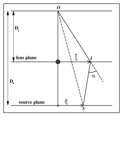
FIG. 1.: The lensing problem in standard gravitational lensing. The point $O$ represents the observer. The point $S$ represents the source. The lens mapping can be interpreted as a map that takes the point $I$ in the lens plane into the point $S$ in the source plane.

FIG. 2.: Diagram of image distortion. The source’s worltube intersects the observer’s past lightcone in a region free of caustics. The source’s visible shape is defined by the intersection. The pencil of rays between the source’s shape and the observer carries the shape of the source into the shape of the image, on the observer’s celestial sphere. The pencil of rays can be described by geodesic deviation vectors (connecting vectors of the observer’s lightcone) from a central null ray connecting the center of the source’s shape to the observer.

FIG. 3.: Vectors associated with the null geodesic that joins the source to the observer. The vector $\ell$ is tangent to the null geodesic. The vectors $(e_{1},e_{2})$ are spacelike, orthogonal to $\ell$, orthonormal and parallel progagated along the geodesics. The vectors $(M_{1},M_{2})$ are linearly independent Jacobi fields which coincide with $(e_{1},e_{2})$ at the location of the source (not shown).

REFERENCES

- [1] P. Schneider, J. Ehlers, and E. E. Falco, Gravitational Lenses (Springer-Verlag, New York, 1992).
- [2] S. Frittelli, T. P. Kling, and E. T. Newman, Image distortion in non-perturbative gravitational lensing, 2000, preprint.
- [3] R. Penrose, in Perspectives in Geometry and Relativity, edited by B. Hoffmann (Indiana University Press, Bloomington, 1966), p. 259.
- [4] R. Blandford et al, MNRAS 251, 600 (1991)
- [5] S. W. Hawking and G. F. R. Ellis, The large-scale structure of spacetime (Cambridge University Press, Cambridge, 1973).
- [6] R. Penrose and W. Rindler, Spinors and Space-time (Cambridge University Press, Cambridge, 1984), Vol. II.
- [7] C. N. Kozameh and E. T. Newman, in Asymptotic Behavior of Mass and Spacetime Geometry, edited by F. J. Flaherty (Springer-Verlag, New York, 1984).
- [8] S. Frittelli, C. N. Kozameh, and E. T. Newman, J. Math. Phys. 36, 6397 (1995).
- [9] S. Frittelli, E. T. Newman, and G. Silva-Ortigoza, Classical and Quantum Gravity 15, 689 (1998).
- [10] S. Frittelli, C. N. Kozameh, and E. T. Newman, J. Math. Phys. 36, 4984 (1995).
- [11] J. Ehlers, S. Frittelli, and E. T. Newman, Gravitational lensing from a spacetime perspective, contribution to the Festschrift in honor of John Stachel, edited by Juergen Renn, submitted March 1999.
- [12] S. Frittelli and E. T. Newman, Phys. Rev. D. 59, 124001/(5) (1999).
- [13] S. Frittelli, T. P. Kling, and E. T. Newman, Phys. Rev. D 61, 064021(14) (2000).
- [14] S. Frittelli, E. T. Newman, and G. Silva-Ortigoza, J. Math. Phys. 40, 383 (1999).
- [15] S. Frittelli, E. T. Newman, and G. Silva-Ortigoza, J. Math. Phys. 40, 1041 (1999).
- [16] V. Perlick, in Einstein’s field equations and their physical implications (Springer, New York, 2000).
- [17] V. Perlick, talk presented at the Gravitational Lensing parallel session of the Ninth Marcel Grossman Meeting, Rome, July 2-8, 2000.
- [18] K. Rauch and R. Blandford, ApJ 421, 46 (1994).
- [19] V. F. Panov and Yu. G. Sbytov, Sov. Phys. JETP 74, 411 (1992).
- [20] D. M. Wittman et al., Detection of weak gravitational lensing distortions of distant galaxies by cosmic dark matter at large scales, astro-ph/0003014 v4.
- [21] R. D. Blanford and M. Jaroszyński, Astrop. J. 246, 1 (1981).