To appear in Phys. Rev. D (January 2001)
Image distortion in non-perturbative gravitational lensing

Abstract

We introduce the idea of shape parameters to describe the shape of the pencil of rays connecting an observer with a source lying on his past lightcone. On the basis of these shape parameters, we discuss a setting of image distortion in a generic (exact) spacetime, in the form of three distortion parameters. The fundamental tool in our discussion is the use of geodesic deviation fields along a null geodesic to study how source shapes are propagated and distorted on the path to an observer. We illustrate this non-perturbative treatment of image distortion in the case of lensing by a Schwarzschild black hole. We conclude by showing that there is a non-perturbative generalization of the use of Fermat’s principle in lensing in the thin-lens approximation.

I Introduction

Before we describe the ideas and content of this work, we wish to give a brief discussion of certain ideas concerning lensing that are really quite obvious but are often overlooked and or confused. It is absolutely clear that any source of light emits many rays that travel in many directions and get distorted by all the different available lenses. But for an observer, of all those different rays, the only ones of relevance are the rays that enter the observers “eyes;” all the others are “lost” to that observer and play no role at all in his or her treatment of lensing. The conclusion from this is that at any one time, it is the past lightcone of the observer that is the object to be studied and understood. It is the bending and distortions of the rays and pencils of rays lying on this past cone that constitute the basic elements that make up lensing theory. When this past cone intersects a source, that source is then seen by the observer; if it is a point source then ideally only one ray reaches the observer, if it is a small but finite source then a pencil of rays, lying on the past cone, reaches the observer. In this later case the pencil can be described by the geodesic deviation vectors (or Jacobi field) associated with just one ray. The shape of the pencil can and will, in general, undergo changes due to the presence of gravitational field along the path of the one ray. It is this change in the shape of the pencil, between the source and the observer, that constitutes image distortion. This is the point of view that we adopt throughout this paper – though the details are very different, the point of view concerning the essential role of the past cone applies equally well to the thin lens approximation (the standard approach) and to the non-perturbative approach to lensing.

It is often the case in gravitational lensing that the distortion of extended images provides as much information to the practicing astrophysicist as the location of the images themselves [1]. In previous work [2, 3, 4], the theory of gravitational lensing has been developed and studied from a first principles point of view, where lensing is considered non-perturbatively with no restrictions on the strength of the gravitational field. This work is non-perturbative in the sense that the key equations of lensing theory, the lens and time of arrival equations, are derived by integrating (as far as possible) the null geodesic equations of an (in principle) exact metric. This point of view is in contrast to the more standard work in lensing based on the thin lens approximation where lenses “live” in some fixed background spacetime. In the present paper and its companion [5], we turn our attention to the non-perturbative study of distortion of images due to lensing.

Images are distorted by a lens in multiple ways. First, an image may be magnified or demagnified, relative to what the image would look like “in the absence of the lens.” Magnification is due to the focusing of the lightcone by the spacetime curvature, and the study of magnification is closely related to catastrophe optics and singularity theory [6, 7, 10, 11, 12, 13]. The magnification of images has proved to be an extremely useful property of lensing systems because it often allows for the observation of very distant sources which may not have been observed without the magnification.

Perhaps more importantly, an extended image may be stretched along some axis, rotated, or made generally larger or smaller relative to an “unlensed image.” Colloquially, we say that the stretching along an axis and rotation of an image is related to the “shearing” of the pencil of light and that an overall change in size is due to the “convergence” (or alternatively, “expansion” or “divergence”) of the pencil. These effects are very important in lens modeling, as the distortion of an extended image into an arc or of identifiable parts of an image (such as the radio jets of a QSO) provides very useful observational constraints on the lens model.

In general relativity, the shear and the convergence are precisely defined quantities [14] which have values at each point along a geodesic. These quantities, often refered to as the optical scalars, have been widely studied in the relativity community. Hence, the general use of these terms in lensing, where an image – observed here – of a source – over there – is said to be “sheared” can be a little misleading.

One goal of this paper and its companion is to propose a unified framework for the non-perturbative discussion of the distortion of images which can be applied in strong-field regimes. In this paper, we introduce three quantities, the shape parameters, describing the generic appearance of an elliptical image or source and show how the shape parameters are computed from connecting vectors. We also introduce three distortion parameters which correspond to changes in the shape parameters between the source and observer. In the following paper, we relate the shape and distortion parameters to the optical scalars.

This paper begins by reviewing the standard (thin-lens) approach to the distortion of images as presented in [15]. In Sec. II, we introduce the key idea of using the inverse Jacobian of the lens equations to map source curves (the outline or boundary of sources) into image curves. We define the shape parameters at the end of this section and briefly mention the quantities which are referred to as the “shear” and “convergence” in the thin lens approximation. (The full discussion of these quantities is left to the second paper, which is devoted to the relationship between the shape parameters and optical scalars.) In the third section of this paper, we present the non-perturbative version of the shape parameters and define the distortion of images. This section relies heavily on the use of connecting vectors or Jacobi fields (we follow the lead of other authors in the use of Jacobi fields in lensing, in particular [8, 9]). The distortion of images in Schwarzschild spacetime is discussed at the conclusion of this section. Finally, we provide a different perspective on the subject in Sec. IV which we feel clarifies several issues regarding the role of the choice of coordinates.

An important caveat must be stated. In a generic lensing situation, if the past lightcone is continued arbitrarily far into the past, caustics will always be found. We, in this work, are making the assumption that our source that is being imaged does not intersect a caustic curve. The morphology of image construction for sources which lie across a caustic is well understood but relatively complicated. The issue of distortion of images in this case is something for further study.

II Image distortion via the thin lens approximation

In this section we summarize the approach to image distortion in standard gravitational lensing according to [15]. The assumptions of the thin lens approximation are that the source, lens, and observer are at rest in the background spacetime, that the gravitational fields are weak, that all angles are small, and that the mass distribution of the entire lens can be collapsed into a single two-dimensional “lens plane” and is described by a surface mass-density, $\kappa(\vec{\xi})$. As is shown in Fig. 1, light rays are assumed to travel along the null geodesics of the background spacetime from a point in the source plane at $S$ to a point in the lens plane (the plane containing the lens and perpendicular to the optical axis) at $I$. At $I$, the ray is instantaneously bent by a bending angle, $\alpha$, and travels to the observer $O$ along another background geodesic. A goal of the thin lens approximation is to find a set of equations, called lens equations, which represent the path of the light ray as a mapping between the lens plane and the source plane.

The lens plane is described by the two dimensional vector $\vec{\xi}$, and the source plane is described by the two dimensional vector $\vec{\eta}$. It is convenient to introduce two scaled vectors

$$\vec{x}=\frac{\vec{\xi}}{D_{l}},\quad\quad\text{and}\quad\quad\vec{y}=\frac{\vec{\eta}}{D_{s}},$$ (1)

which describe the lens $(\vec{x})$ and source $(\vec{y})$ planes. Here $D_{s}$ and $D_{l}$ are the angular-diameter distances between the observer and source and observer and lens.

The dynamics of the thin lens approximation is introduced through a deflection potential

$$\psi(\vec{x})=\frac{1}{\pi}\int_{\mbox{R}^{2}}\,dx^{\prime 2}\kappa(\vec{x}^{\prime})\ln|\vec{x}-\vec{x}^{\prime}|,$$ (2)

where $\kappa(\vec{x})$ is the surface mass-density, satisfying the two-dimensional Laplace equation

$$\nabla^{2}\psi(\vec{x})=2\kappa(\vec{x}).$$ (3)

The lens mapping from the lens plane to the source plane, or from $\vec{x}$ to $\vec{y}$, is a gradient mapping:

$$\vec{y}=\nabla\left(\frac{1}{2}\vec{x}\cdot\vec{x}-\psi(\vec{x})\right),$$ (4)

or,

$$\vec{y}=\vec{x}-\nabla\psi(\vec{x}).$$ (5)

Equation (4) is the lens equation of the thin-lens approximation under the scaling defined by Eqs. (1).

An alternative perspective is to derive the lens equation, Eq. (4), by applying a stationarity condition to a Fermat potential. If we define

$$\widehat{\phi}(\vec{y},\vec{x})=\frac{1}{2}(\vec{x}-\vec{y})^{2}-\psi(\vec{x}),$$ (6)

as a Fermat potential, the gradient mapping is equivalent to the condition

$$\nabla_{x}\widehat{\phi}(\vec{y},\vec{x})=0,$$ (7)

i.e., the lens equation, Eq. (5), follows from Fermat’s principle. (We generalize the idea of a Fermat potential in Sec. IV to a general lensing scenario, noting that other authors have also studied this problem extensively [16].) Note that the second derivativeof $\hat{\phi}(\vec{y},\vec{x})$ with respect to $\vec{x}$ is equal tothe derivative of $\vec{y}$ with respect to $\vec{x}$ as defined inEq. (4).

The distortion of images can be studied via the Jacobian of the lens mapping

$$\mbox{\boldmath$A$}\equiv\frac{\partial\vec{y}}{\partial\vec{x}}=\frac{\partial^{2}\widehat{\phi}}{\partial\vec{x}\partial\vec{x}}.$$ (8)

We see that the Jacobian matrix is symmetric. This symmetry exists, essentially, only in the special coordinates used. We will see in Sec. IV how this result arises non-perturbatively.

Using the lens equation, Eq. (4), we see that the Jacobian matrix has the form

$$\mbox{\boldmath$A$}=\left(\begin{array}[]{cc}1-\psi_{11}&-\psi_{12}\\ -\psi_{21}&1-\psi_{22}\end{array}\right),$$ (9)

where subscripts denote derivatives with respect to the components of $\vec{x}=(x^{1},x^{2})$. By defining

$$\gamma_{1}(\vec{x}) \equiv \frac{1}{2}(\psi_{11}-\psi_{22}),$$ (10)

$$\gamma_{2}(\vec{x}) \equiv \psi_{12}=\psi_{21}$$ (11)

and using Eq. (3), we can rewrite the Jacobian matrix as

$$\mbox{\boldmath$A$}=\left(\begin{array}[]{cc}1-\kappa-\gamma_{1}&-\gamma_{2}\\ -\gamma_{2}&1-\kappa+\gamma_{1}\end{array}\right),$$ (12)

where we have dropped the explicit $\vec{x}$ dependence in $\kappa(\vec{x})$, $\gamma_{1}(\vec{x})$ and $\gamma_{2}(\vec{x})$.

It has become customary in the lensing community [15, 17] to refer to $\kappa$ as the convergence, and $\gamma\equiv\sqrt{\gamma_{1}^{2}+\gamma_{2}^{2}}$ as the shear . In this and the subsequent paper [5], however, we will reserve the names of convergence and shear for the optical scalars of a null geodesic congruence. We show in our subsequent paper that (modulo terms involving $D_{s}$ and $D_{l}$) $\kappa$ and $\gamma$ are essentially the values of the convergence and shear of the observer’s past lightcone at the lens plane on the source’s side.

In terms of $\kappa$ and $\gamma$, the invariants of $A$ are

$$\det\mbox{\boldmath$A$} = (1-\kappa)^{2}-\gamma^{2}$$ (13)

tr $$A = 2(1-\kappa)$$ (14)

$$a_{\pm} = 1-\kappa\pm\gamma$$ (15)

where $a_{\pm}$ are the eigenvalues of the Jacobian matrix. When $\det\mbox{\boldmath$A$}=0$, the lens mapping is singular and the source lies at a caustic of the past cone. The quantity $\mu=(\det\mbox{\boldmath$A$})^{-1}$, referred to as the magnification, is the factor by which the image’s brightness is magnified with respect to the unlensed source.

Another important use of the Jacobian is to help understand the changes in the shape of the image of a small source. To see this, we note that a (suitably scaled) connecting vector, $\vec{X}$, at $\vec{x}$ in the lens plane, is mapped into a (suitably scaled) connecting vector, $\vec{Y}$, at $\vec{y}$ in the source plane, by $A$, while $\mbox{\boldmath$A$}^{-1}$ maps source plane vectors back to the lens plane:

$$\vec{Y}=\mbox{\boldmath$A$}\vec{X}.$$ (16)

For instance, if a small circle of radius $R$ at $\vec{y}$ in the source plane is described by

$$\vec{Y}(t)=\vec{y}+R\,\vec{s}(t)$$ (17)

where $\vec{s}(t)=(\cos t,\sin t)$, an image of this circle is an ellipse, in the lens or image plane, described by

$$\vec{X}(t)=\vec{x}+R\,\mbox{\boldmath$A$}^{-1}\vec{s}(t)$$ (18)

Hence, the Jacobian matrix, $A$, and its inverse, $\mbox{\boldmath$A$}^{-1}$, which is referred to as the magnification matrix, play a large role in the description of the images of small sources.

The semiaxes of the ellipse described by Eq. (18) must be parallel to the principal axes of the magnification matrix $\mbox{\boldmath$A$}^{-1}$, which are the same as the principal axes of $A$. This is because there are two vectors $\vec{s}(t_{\pm})=(\cos t_{\pm},\sin t_{\pm})$, which are parallel to the two eigenvectors of $A$ and are mapped into themselves by $A$ and $\mbox{\boldmath$A$}^{-1}$. These two directions undergo the maximum stretching and squeezing because the eigendirections of a symmetric linear map are those which have the greatest and least stretching. Hence, the lengths of the major and minor semiaxes are

$$L_{\pm}=\frac{R}{|1-\kappa\mp\gamma|}.$$ (19)

The locations of these axes are given by the angles, $t_{\pm}$, which satisfy

$$\tan t_{\pm}=\frac{\gamma_{1}}{\gamma_{2}}\mp\sqrt{\left(\frac{\gamma_{1}}{\gamma_{2}}\right)+1},$$ (20)

i.e., in the directions

$$\vec{X}(t_{\pm})=\vec{x}+R\mbox{\boldmath$A$}^{-1}\vec{s}(t_{\pm}).$$ (21)

This result is obtained [via extremizing $(\vec{X}(t)-\vec{x})^{2}$ as a function of $t$] by finding the angles, $t$, for vectors of the form of $\vec{s}(t)=(\cos t,\sin t)$ which are the eigenvectors.

We are now in the position to define our shape parameters. The first shape parameter is the ratio of the lengths of the semimajor and semiminor axes, ${\cal R}$. This ratio is given by

$${\cal R}=\frac{L_{+}}{L_{-}}=\frac{|1-\kappa+\gamma|}{|1-\kappa-\gamma|}$$ (22)

in the thin-lens approximation. The second shape parameter is the area of the ellipse factored by $\pi$, or the product of the two semiaxes, which we refer to as the area of the ellipse (since the area is proportional to the product of the semiaxes with a factor of $\pi$). For the thin lens approximation, the (factored) area is given by

$${\cal A}\equiv L_{+}L_{-}=\frac{R^{2}}{(1-\kappa)^{2}-\gamma^{2}}=R^{2}\det(\mbox{\boldmath$A$}^{-1})$$ (23)

The final shape parameter is the orientation of the major semiaxis, $\delta$. By convention, we define $\delta$ to be $\delta\equiv t_{+}$.

Thus, there are three quantities of interest in describing the image of a circular source: the (suitably scaled) area of the image $\cal A$, which encodes the overall scaling of the image compared to the source; the ratio of the semiaxes $\cal R$ which is a measure of the distortion up to scale; and the orientation of the semimajor axis $\delta\equiv t_{+}$. This definition of the orientation does not have a definite meaning without a reference axis or when referred to a circular source but it can be assigned a meaning for an elliptical source when the discussion is generalized slightly as will be done later in this article. We refer to these three quantities as the shape parameters. They will be defined non-perturbatively in the next section.

III Non-perturbative image distortion

We are interested in understanding image distortion within general relativity with no approximations. We refer to this approach to image distortion as a non-perturbative approach, to distinguish it from the standard approach which is based on linearized perturbations around flat space or an isotropic cosmological model.

To this effect, we need two things. First, we need a non-perturbative counterpart of the lens mapping. Once the lens mapping is given, the Jacobian matrix, or its inverse, the magnification matrix, can be obtained. Second, we need non-perturbative definitions for image and source shapes, and distortion parameters, which encode the changes between the shapes of the source and the image, in terms of the magnification matrix.

A Lens mapping

At any fixed time the observer “sees” each source (on his or her past lightcone) projected onto the observer’s celestial sphere. By introducing spherical coordinates, $(\theta,\phi)$, for each ray, via this projection, the observer encodes a mapping between an image location, $(\theta,\phi)$, and a source location. A formal lens mapping can be obtained by the following considerations, summarized from [2, 3]. Similar considerations have been studied recently by other authors [18, 19]. In particular, see [20] for exact lensing in Kerr spacetime.

In a four dimensional Lorentzian space-time, $({\cal M},g_{ab}(z^{a}))$, with local coordinates $z^{a}$, we assume that an expression for the past lightcone of the observer, obtained by integrating the null geodesic equations, is available. It has the form of four functions of three parameters of the light cone at an observer’s fixed time, $\tau$:

$$z^{a}=F^{a}(z_{0}^{b}(\tau),s,\theta,\phi).$$ (24)

Here $z^{a}$ represents a point on the past lightcone of the observer’s worldline, $z_{0}^{b}(\tau)$ at time $\tau$, reached at an affine length $s$ along the null geodesic with direction $(\theta,\phi)$. The affine length $s$ has the value zero at the observer and is scaled so that $g_{ab}\dot{F}^{a}\dot{z}_{0}^{b}=1$, using the notation $\dot{\;}\equiv\frac{\partial}{\partial s}$. Thefunctions $F^{a}$ can be obtained by integrating the geodesic equations, $\ddot{F}^{a}+\Gamma_{bc}^{a}\dot{F}^{b}\dot{F}^{c}=0$ with the null condition

$$g_{ab}\dot{F}^{a}\dot{F}^{b}=0.$$ (25)

The coordinates are arbitrary, but they can be chosen so that one of them, say $z^{0}$, is timelike and the remaining three $z^{i}$ are spacelike, i=1,2,3. In this case, for $a=0$, Eq. (24) represents the time of departure of a light signal from the source to the observer. On the other hand, Eq. (24) for $a=1,2,3$ is equivalent to a lens mapping between the angular position, $(z^{2},z^{3})$, say, of a source of light and its image angles $(\theta,\phi)$ on the observer’s celestial sphere, plus a prescription of a radial coordinate, $z^{1}$, which, in principle, can be obtained from independent observations. Ideally, if the radial coordinate is known as a function of the affine parameter $s$, then, in principle, the parameter $s$ can be eliminated from $F^{A}(s,\theta,\phi)$, for $A=2,3$, in terms of $(z^{1},\theta,\phi)$, in which case a precise analog of the standard lens mapping is obtained of the form $z^{A}=G^{A}(z^{1},\theta,\phi)$. For our purposes, it is not essential to eliminate $s$, which may not even be possible in general (see [4] for the feasibility of such an elimination in the simple case of a Schwarzschild spacetime). The non-perturbative lens mapping $z^{A}=G^{A}(z^{1},\theta,\phi)$ has been worked out explicitly in the case of a Schwarzschild spacetime [4] and compared to standard lensing.

Aside. Our non-perturbative version of a lens mapping differs from the standard lens mapping, in addition to being non-perturbative, in the sense that we do not use explicitly the Einstein equations – we simply consider any Lorentzian metric $g_{ab}(z^{a})$ and its null geodesics to construct the observer’s past cones and the resulting lens equation. In most thin-lens treatments of lensing the linearized Einstein equations (in the form $\nabla^{2}\psi(\vec{x})=2\kappa(\vec{x})$) are used explicitly from the start in the construction of the lens equation.

B Jacobian of the Lens Mapping

Consider the situation where there is an extended source at some distance from an observer. The source’s worldtube intersects the observer’s past lightcone, and we assume that the intersection occurs in a region of the past lightcone where there are no caustics. See Fig. 2. The intersection determines the source’s visible shape. The pencil of rays that joins the shape of the source to the observer “carries” the shape of the source into the shape of the image, on the observer’s celestial sphere. For the lensing purposes, thus, an extended source consists of a collection of individual point sources, all of which are connected to the observer by individual null geodesics. In general, the image of an extended source must be obtained by imaging each individual point via the non-perturbative lens equation. However, if the sources are “small,” we can, in the spirit of the previous Section, describe sources by connecting vectors along one of the null geodesics (a “central” one), with image directions $(\theta,\phi)$, that joins the source to the observer. Jacobi fields (or connecting vectors) are solutions to the geodesic deviation equation along that fixed geodesic. In the case of null geodesics, the space of Jacobi fields is two-dimensional and can be obtained in our approach directly from our non-perturbative lens mapping Eq. (24) in the following manner.

We note that there are three natural vectors that can be associated with either the past lightcone or equivalently with the lens equation, Eq. (24). The first one is the tangent to the geodesics in the lightcone:

$$\ell^{a}\equiv\frac{\partial z^{a}}{\partial s}=\dot{F}^{a}.$$ (26)

The remaining two are the Jacobi fields

$$\widetilde{M}_{1}^{a}\equiv\frac{\partial z^{a}}{\partial\theta},\hskip 42.67912pt\widetilde{M}_{2}^{a}\equiv(\sin\theta)^{-1}\frac{\partial z^{a}}{\partial\phi}.$$ (27)

These two vectors are, in general, linearly independent and connect neighboring geodesics at a fixed value of $s$, so they are two linearly independent Jacobi fields (except at a caustic). They are orthogonal to the tangent vector $\ell^{a}$ because they lie on the lightcone: $g_{ab}\widetilde{M}_{1}^{a}\ell^{b}=g_{ab}\widetilde{M}_{2}^{a}\ell^{b}=0$, and they are spacelike. Though any other Jacobi field is a linear combination of $(\widetilde{M}_{1}^{a},\widetilde{M}_{2}^{a})$ with constant parameters $\alpha,\beta$,

$$Z^{a}=\alpha\widetilde{M}_{1}^{a}+\beta\widetilde{M}_{2}^{a},$$ (28)

we refer to $(\widetilde{M}_{1}^{a},\widetilde{M}_{2}^{a})$ as the “natural” Jacobi fields.

Two other important vector fields (not Jacobi fields) associated with any null geodesic are the pair of spacelike, orthonormal, parallel propagated vectors that are normal to $\ell^{a}$. They provide a means to refer to directions that are “the same” at the orthogonal tangent spaces at the source and at the observer. Analytically they are given by

$$\ell^{b}\nabla_{\!b}e_{1}^{a} = \ell^{b}\nabla_{\!b}e_{2}^{a}=0,$$ (29)

$$e_{1}\!\cdot\ell = e_{2}\!\cdot\ell=0,$$ (30)

$$e_{1}\!\cdot e_{1} = e_{2}\!\cdot e_{2}=-1,$$ (31)

$$e_{1}\!\cdot e_{2} = 0,$$ (32)

where $v\!\cdot\!w$ denotes the scalar product between two vectors, $g_{ab}v^{a}w^{b}$.

The natural connecting vectors, $(\widetilde{M}_{1}^{a},\widetilde{M}_{2}^{a})$, in general, will have transverse components along the space spanned by $(e_{1}^{a},e_{2}^{a})$, and a longitudinal component along the geodesic congruence $\ell^{a}$. The component along $\ell^{a}$ has no significance since it corresponds to reparametrizations of the null geodesic. Jacobi fields thus have two essential transverse components. Two linearly independent Jacobi fields can thus be thought as two two-component vectors that are obtained by derivation from the lens mapping. Explicitly, this can be done by the projection of $(\widetilde{M}_{1}^{a},\widetilde{M}_{2}^{a})$ into $(e_{1}^{a},e_{2}^{a})$, thereby defining the matrix $\widetilde{\mbox{\boldmath$J$}}(s)$

$$(\widetilde{M}_{1}^{a},\widetilde{M}_{2}^{a})\rightarrow\left[\widetilde{\mbox{\boldmath$J$}}(s)\right]\equiv\widetilde{\mbox{\boldmath$J$}}_{i}^{j}(s)=\widetilde{M}_{i}^{a}e_{a}^{j}.$$ (33)

At the observer (i.e., at the apex of the cone), the connecting vectors $(\widetilde{M}_{1}^{a},\widetilde{M}_{2}^{a})$ vanish, so that $\widetilde{\mbox{\boldmath$J$}}(0)=0$, and, furthermore, in the limit as $s\rightarrow 0$ we have that

$$\lim_{s\to 0}\frac{1}{s}\widetilde{\mbox{\boldmath$J$}}(s)=\mbox{\boldmath$I$}$$ (34)

where $I$ is the identity matrix. This last result is quite important and comes from the fact that although the connecting vectors vanish at $s=0,$ their angular size has been chosen to be unity. (At each value of $s$ close to the observer, each connecting vector subtends an arc from the observer’s viewpoint. The connecting vector’s arc is proportional to $s$, therefore the angular size of the connecting vector at the observer is well defined, and equal to the derivative of the connecting vector with respect to $s$.)

We adopt the following notation. When the matrix $\widetilde{\mbox{\boldmath$J$}}(s)$ is evaluated at the source position, denoted by $s=s^{*}$, it is called the Jacobian of the lens mapping and is denoted by ${}^{*}\!\!\widetilde{J}$. In addition, we denote any quantity that is defined or evaluated at the source by placing a ^∗ in front of it, e.g., $({}^{*}\!\widetilde{M}_{1}^{a},{}^{*}\!\widetilde{M}_{2}^{a})=(\widetilde{M}_{1}^{a}(s^{*}),\widetilde{M}_{2}^{a}(s^{*}))$.

Notice that, in a weak field-thin lens regime, our Jacobian ${}^{*}\!\!\widetilde{J}$ is related to the Jacobian $A$ of the thin-lens theory via

$$\mbox{\boldmath$A$}=\frac{\mbox{\boldmath${}^{*}\!\!\widetilde{J}$}}{s^{*}}$$ (35)

We now put a source at $s^{*}$ with an elliptical shape and study how it is mapped back to the image space,the observer’s celestial sphere. Though it is possible to do this construction with $(\widetilde{M}_{1}^{a}(s),\widetilde{M}_{2}^{a}(s))$ (or,equivalently, with $\widetilde{\mbox{\boldmath$J$}}_{i}^{j}(s)$) it turns out to be considerably simpler to use a pair of Jacobi fields, $(M_{1}^{a},M_{2}^{a})$, constructed from a linear combination of the $\widetilde{M}_{i}^{a}$ that are unit orthogonal vectors at $s=s^{*}$, i.e., so that $\mbox{\boldmath$J$}_{i}^{j}(s)\equiv M_{i}^{a}e_{a}^{j}$ is the identity matrix at $s=s^{*}$:

$$\mbox{\boldmath$J$}_{i}^{j}(s^{*})\equiv{}^{*}\!M_{i}^{a}{}^{*}\!e_{a}^{j}=\delta_{i}^{j}.$$ (36)

It is easy to see that the linear combination must have the form

$$M_{i}^{a}=(\mbox{\boldmath${}^{*}\!\!\widetilde{J}$}^{-1})_{i}^{j}\widetilde{M}_{j}^{a},$$ (37)

so that

$$M_{i}^{a}e_{a}^{k}=(\mbox{\boldmath${}^{*}\!\!\widetilde{J}$}^{-1})_{i}^{j}\widetilde{M}_{j}^{a}e_{a}^{k}\quad\Rightarrow\mbox{\boldmath$J$}_{i}^{k}(s)=(\mbox{\boldmath${}^{*}\!\!\widetilde{J}$}^{-1})_{i}^{j}\widetilde{\mbox{\boldmath$J$}}_{j}^{k}(s),$$ (38)

and hence

$$\mbox{\boldmath$J$}_{i}^{k}(s^{*})=(\mbox{\boldmath${}^{*}\!\!\widetilde{J}$}^{-1})_{i}^{j}\mbox{\boldmath${}^{*}\!\!\widetilde{J}$}_{j}^{k}=\delta_{i}^{k}.$$ (39)

This is equivalent to assuming that we have chosen two connecting vectors $M_{1}^{a}$ and $M_{2}^{a}$ so that

$${}^{*}\!M_{1}^{a} = {}^{*}\!e_{1}^{a},$$ (40)

$${}^{*}\!M_{2}^{a} = {}^{*}\!e_{2}^{a}.$$ (41)

In general, the two pairs $(M_{1}^{a},M_{2}^{a})$ and $(e_{1}^{a},e_{2}^{a})$, coincide at the point $s^{*}$, but not at any other point along the null geodesic. See Fig. 3.

For our construction in this article, it is a fundamental observation that, from Eqs. (38) and (34), as $s\to 0$ we have

$$\frac{1}{s}\mbox{\boldmath$J$}(s)\to\mbox{\boldmath${}^{*}\!\!\widetilde{J}$}^{-1},$$ (42)

i.e., in the limit as the null geodesic reaches the observer, $J$ acts essentially as the inverse of the Jacobian of the lens map, namely, as our magnification matrix. We make extensive use of this result throughout this and the companion paper [5].

Preliminarily to defining the shape and distortion parameters we point out that even though the pairs $(e_{1}^{a},e_{2}^{a})$ and $(M_{1}^{a},M_{2}^{a})$ possess different meanings from each other, they can nevertheless be expressed as linear combinations of each other. Assuming a relationship of the form

$$e_{1}^{a} = \alpha\cos(\lambda+\nu)M_{1}^{a}+\beta\cos\lambda M_{2}^{a},$$ (43)

$$e_{2}^{a} = \alpha\sin(\lambda+\nu)M_{1}^{a}+\beta\sin\lambda M_{2}^{a},$$ (44)

and using the properties of $e_{i}^{a}$ and its dual basis, namely

$$e_{i}^{a}e_{a}^{j}=\delta_{i}^{j},\qquad e_{i}^{a}\ell_{a}=0,\qquad\ell^{b}\nabla_{\!b}e_{i}^{a}=0$$ (45)

after a straightforward calculation the four parameters $(\alpha,\beta,\nu,\lambda,)$ can be obtained in terms of the scalar products $M_{1}\!\cdot M_{1},M_{2}\!\cdot M_{2}$ and $M_{1}\!\cdot M_{2}$ as follows:

$$\alpha = \sqrt{\frac{-M_{2}\!\cdot\!M_{2}}{C}},$$ (46)

$$\beta = \sqrt{\frac{-M_{1}\!\cdot\!M_{1}}{C}},$$ (47)

$$\cos\nu = \frac{M_{1}\!\cdot\!M_{2}}{\sqrt{M_{1}\!\cdot\!M_{1}M_{2}\!\cdot\!M_{2}}},$$ (48)

where we use, for short,

$$C\equiv M_{1}\!\cdot M_{1}M_{2}\!\cdot\!M_{2}-(M_{1}\!\cdot\!M_{2})^{2},$$ (49)

and

$$\dot{\lambda}=\frac{M_{1}\!\cdot\!M_{2}}{2\sqrt{C}}\frac{d}{ds}\log\left(\frac{M_{2}\!\cdot\!M_{2}}{M_{1}\!\cdot\!M_{2}}\right).$$ (50)

which fixes $\lambda$ up to a constant. The quantity $C$ represents the area spanned by $(M_{1}^{a},M_{2}^{a})$, i.e., $C=g^{ad}n_{a}n_{d}$ with $n_{a}\equiv\epsilon_{abc}M_{1}^{b}M_{2}^{c}$.

Notice that the values of $(\alpha,\beta,\nu,\lambda)$ at $s^{*}$ are determined to be

$${}^{*}\!\alpha=1,\hskip 28.45274pt{}^{*}\!\beta=1,\hskip 28.45274pt{}^{*}\!\nu=-\frac{\pi}{2},\hskip 28.45274pt{}^{*}\!\lambda=\frac{\pi}{2}.$$ (51)

We thus have the orthonormal parallel propagated basis written in terms of the Jacobi fields.

C Shape and distortion parameters

We now discuss the source parameters that enter into the considerations of image distortion. Specifically we consider small elliptical sources, which can be completely described by three parameters: the lengths of the two semiaxes, and the orientation of, say, the major semiaxis with respect to a reference direction. The two semiaxes can be equivalently encoded into the ratio of major to minor semiaxis, and the product of the two. The product of the two semiaxes is the area of the ellipse divided by the number $\pi$. In order to avoid carrying the factor $\pi$ around, in this paper, we simply refer to the product of the two semiaxes as the area of the ellipse and denote it by ${}^{*}\!\!{\cal A}$. We denote the ratio of the semiaxes by ${}^{*}\!{\cal R}$, and the orientation of the major semiaxis with respect to the parallel propagated direction $e_{1}^{a}$ by ${}^{*}\!\delta$. These are, by definition, our shape parameters evaluated at the source, $s^{*}$.

At the source location, we have an orthonormal basis, $({}^{*}\!e_{1}^{a},{}^{*}\!e_{2}^{a})$, in terms of which an ellipse can be expressed as

$${}^{\ast}\!Y^{a}(t)\equiv Y^{1}(t)^{*}e_{1}^{a}+Y^{2}(t)^{*}e_{2}^{a}=Y^{1}(t)^{*}M_{1}^{a}+Y^{2}(t)^{*}M_{2}^{a}$$ (52)

where the components $Y^{i}(t)$, $t$ being the curve parameter, can be given by

$$\left(\begin{array}[]{c}Y^{1}\\ Y^{2}\end{array}\right) = \left(\begin{array}[]{cc}\cos\!{}^{*}\!\delta&-\sin\!{}^{*}\!\delta\\ \sin\!{}^{*}\!\delta&\cos\!{}^{*}\!\delta\end{array}\right)\left(\begin{array}[]{cc}\sqrt{{}^{*}\!\!{\cal A}^{*}\!{\cal R}}&0\\ 0&\sqrt{{}^{*}\!{\cal A}/{}^{*}\!{\cal R}}\end{array}\right)\left(\begin{array}[]{c}\cos t\\ \sin t\end{array}\right)$$ (61)

$$\equiv \sqrt{{}^{*}\!\!{\cal A}/{}^{*}\!{\cal R}}\left(\begin{array}[]{c}{}^{*}\!{\cal R}\cos t\cos\!{}^{*}\!\delta-\sin t\sin\!{}^{*}\!\delta\\ {}^{*}\!{\cal R}\cos t\sin\!{}^{*}\!\delta+\sin t\cos\!{}^{*}\!\delta\end{array}\right)$$ (64)

As indicated, this arises from first taking a parametrized circle (the vector $(\cos t,\sin t)$), then distorting into an ellipse of major semiaxis $\sqrt{{}^{*}\!\!{\cal A}{}^{*}\!{\cal R}}$ (the product of the semiaxes times the ratio of major to minor is the square of the major axis) and minor semiaxis $\sqrt{{}^{*}\!{\cal A}/{}^{*}\!{\cal R}}$ (the product of the semiaxes over the ratio of major to minor is the square of the minor axis) and finally rotating through an arbitrary angle ${}^{*}\!\delta$.

Remark: One should not confuse the curve parameter $t$ with the polar angle$\phi$ of each corresponding point on the curve relative to the direction ${}^{*}\!e_{1}^{a}$. The polar angle $\varphi$ is related to $t$ at the source by $\tan(\varphi-\delta_{*})=\tan t/{}^{*}\!{\cal R}$.

In order to obtain the image of this source, we “follow” each point of the ellipse back towards the observer using the Jacobi fields $M_{i}^{a}(s)$, i.e., via

$$Z^{a}(s,t) \equiv Y^{1}(t)M_{1}^{a}(s)+Y^{2}(t)M_{2}^{a}(s)$$ (65)

$$= \sqrt{\frac{{}^{*}\!\!{\cal A}}{{}^{*}\!{\cal R}}}\Big{(}({}^{*}\!{\cal R}\cos t\cos\!{}^{*}\!\delta-\sin t\sin\!{}^{*}\!\delta)M_{1}^{a}+({}^{*}\!{\cal R}\cos t\sin\!{}^{*}\!\delta+\sin t\cos\!{}^{*}\!\delta)M_{2}^{a}\Big{)}.$$ (66)

The vector field $Z^{a}$ is a Jacobi field for every value of $t$, therefore it describes the image of the source near $s\to 0$, the observer’s location. On the other hand, it agrees with our expression for the source at $s^{*}$, because of Eqs. (40)-(41).

Projecting the components of $Z^{a}(s,t)$ in the $e_{i}^{a}$ directions we have

$$Z^{i}(s,t)\equiv Z^{a}(s,t)e_{a}^{i}=Y^{j}(t)M_{j}^{a}(s)e_{a}^{i}=\mbox{\boldmath$J$}_{j}^{i}(s)Y^{j}(t);$$ (67)

the matrix $J$ thus pulls the source’s shape back towards the observer. We then have the projected image of the source on the observer’s celestial sphere given by

$$X^{i}(t)=\lim_{s\to 0}\frac{1}{s}\mbox{\boldmath$J$}_{j}^{i}(s)Y^{j}(t)=(\mbox{\boldmath${}^{*}\!\!\widetilde{J}$}^{-1})_{j}^{i}Y^{j}(t)$$ (68)

or

$$X(t)=\mbox{\boldmath${}^{*}\!\!\widetilde{J}$}^{-1}Y(t).$$ (69)

This is the non-perturbative equivalent of Eq. (18) of Section II. Notice, however, that we have not scaled the connecting vector at the source. (The connecting vector at the observer must be scaled by $s$ in order for it not to vanish.)

The image $X^{a}(t)$ of the ellipse $Y^{a}(t)$ is an ellipse as well because a non-singular continous linear transformation of an ellipse is also an ellipse. In order to read off the image’s elliptic parameters, we start by extremizing the distance $Z\!\cdot Z$ as a function of the parameter $t$. Directly from Eq. (66) we have

$$Z\!\cdot Z=\frac{{}^{*}\!\!{\cal A}}{{}^{*}\!{\cal R}}\left(a+b\sin^{2}t+c\sin t\cos t\right),$$ (70)

with

$$a(s) = {}^{*}\!{\cal R}^{2}\Big{(}(\cos\!{}^{*}\!\delta)^{2}M_{1}\!\cdot\!M_{1}+(\sin\!{}^{*}\!\delta)^{2}M_{2}\!\cdot\!M_{2}+2\sin\!{}^{*}\!\delta\cos\!{}^{*}\!\delta M_{1}\!\cdot\!M_{2}\Big{)},$$ (71)

$$b(s) = \frac{1}{2}(1-\!{}^{*}\!{\cal R}^{2})(M_{1}\!\cdot\!M_{1}+M_{2}\!\cdot\!M_{2})+\frac{1}{2}(1+\!{}^{*}\!{\cal R}^{2})\cos(2{}^{*}\!\delta)(M_{2}\!\cdot\!M_{2}-M_{1}\!\cdot\!M_{1})-(1+\!{}^{*}\!{\cal R}^{2})\sin(2{}^{*}\!\delta)M_{1}\!\cdot\!M_{2},$$ (72)

$$c(s) = {}^{*}\!{\cal R}\Big{(}\sin(2{}^{*}\!\delta)(M_{2}\!\cdot\!M_{2}-M_{1}\!\cdot\!M_{1})+2\cos(2{}^{*}\!\delta)M_{1}\!\cdot\!M_{2}\Big{)}.$$ (73)

Extremization ($d(Z\!\cdot\!Z)/dt=0$) yields

$$\tan(2t)=-\frac{c}{b}.$$ (74)

There are, thus, four values of $t$ in the interval $[0,2\pi]$ that extremize the distance to the center, and they differ by $\pi/2$. Using Eq. (74), we can obtain, for $Z\!\cdot\!Z$,

$$Z\!\cdot\!Z=\frac{{}^{*}\!\!{\cal A}}{2{}^{*}\!{\cal R}}\left(2a+b\pm\sqrt{b^{2}+c^{2}}\right).$$ (75)

The lengths of the major and minor semiaxes, $L_{+}$ and $L_{-}$, respectively, are thus

$$L_{+} = \left(\frac{{}^{*}\!\!{\cal A}}{2{}^{*}\!{\cal R}}\left(-2a-b+\sqrt{b^{2}+c^{2}}\right)\right)^{1/2},$$ (76)

$$L_{-} = \left(\frac{{}^{*}\!\!{\cal A}}{2{}^{*}\!{\cal R}}\left(-2a-b-\sqrt{b^{2}+c^{2}}\right)\right)^{1/2}.$$ (77)

The ratio of the semiaxes is thus

$${\cal R}=\left(\frac{2a+b-\sqrt{b^{2}+c^{2}}}{2a+b+\sqrt{b^{2}+c^{2}}}\right)^{1/2}$$ (78)

where $a,b,c$ are explicit functions of the scalar products between the two connecting vectors $M_{1}^{a}$ and $M_{2}^{a}$ given by (71)-(73).

The product of the semiaxes is what we refer to as the area of the ellipse

$${\cal A}=\frac{{}^{*}\!\!{\cal A}}{2{}^{*}\!{\cal R}}\big{(}4a(a+b)-c^{2}\big{)}^{1/2}.$$ (79)

With the parameters $a,b$ and $c$ given by Eq. (71), Eq. (72) and Eq. (73) this becomes

$${\cal A}={}^{*}\!\!{\cal A}\Big{(}M_{1}\!\cdot M_{1}M_{2}\!\cdot M_{2}-(M_{1}\!\cdot M_{2})^{2}\Big{)}^{1/2}$$ (80)

as is expected.

In order to find the orientation $\delta$ of the ellipse with respect to $e_{1}^{a}$ we need to express $Z^{a}$ in the basis $(e_{1}^{a},e_{2}^{a})$. This is done by inverting Eqs.(43)-(44), obtaining

$$M_{1}^{a} = \frac{\cos\lambda e_{2}^{a}-\sin\lambda e_{1}^{a}}{\alpha\sin\nu},$$ (81)

$$M_{2}^{a} = \frac{\sin(\lambda+\nu)e_{1}^{a}-\cos(\lambda+\nu)e_{2}^{a}}{\beta\sin\nu},$$ (82)

The orientation $\delta$ is then given by $\tan\delta\equiv(Z\!\cdot e_{2})/(Z\!\cdot e_{1})$, or

$$\tan\delta=\frac{\alpha\cos(\lambda+\nu)({\cal R}_{*}\cos t\sin\delta_{*}+\sin t\cos\delta_{*})-\beta\cos\lambda({\cal R}_{*}\cos t\cos\delta_{*}-\sin t\sin\delta_{*})}{\beta\sin\lambda({\cal R}_{*}\cos t\cos\delta_{*}-\sin t\sin\delta_{*})-\alpha\sin(\lambda+\nu)({\cal R}_{*}\cos t\sin\delta_{*}+\sin t\cos\delta_{*})}.$$ (83)

For generic values of $t$ this yields the polar angle that the points on the ellipse make with the direction $e_{1}^{a}$. The orientation of the semiaxes is obtained by using, for $t$, the values $t_{\pm}$ of Eq. (74). It is straightforward to check that the values of $t_{\pm}$ given by Eq. (74), which differ by $\pi/2$, yield values of $\delta$ that also differ by $\pi/2$, as expected for an ellipse. [Other authors [21] have studied the rotation of the image of an elliptical source but in a different physical context (the appearance of the polarization of radio emission by sources at high redshift).]

We have thus obtained our shape parameters ${\cal R,A}$ and $\delta$ in terms of Jacobi fields, in Eq. (78), Eq. (80) and Eq. (83).

In the limit as $s\to 0$ we can obtain, from these shape parameters, the values of the elliptic parameters of the image. Notice that both ${\cal R}$ and $\delta$ are well defined and finite as $s\to 0$, because they are ratios of connecting vectors that vanish at the same rate (like $s$). Therefore, if we denote the ratio of semiaxes of the image by ${\cal R}_{I}$, and their orientation by $\delta_{I}$, their values are simply the values of ${\cal R}$ and $\delta$ at $s=0$:

$${\cal R}_{I} = {\cal R}(0),$$ (84)

$$\delta_{I} = \delta(0).$$ (85)

The area of the image, however, is not a well-defined concept, since the image lies on the celestial sphere of the observer, which has no definite radius. Furthermore, the shape parameter that gives the area of the pencil or rays, ${\cal A}$, necessarily vanishes at the observer’s location (the apex of the lightcone). Nevertheless, the solid angle of the image (i. e., its “angular” area) is a meaningful concept. In order to obtain the image’s solid angle, we define the solid angle $\Omega(s)$ of the corresponding the pencil of rays:

$$\Omega(s)\equiv\frac{\cal A}{s^{2}}$$ (86)

from which the image’s solid angle $\Omega_{I}$ can be obtained by passing to the limit as $s\to 0$, namely:

$$\Omega_{I}=\lim_{s\to 0}\Omega(s).$$ (87)

We define now the distortion of the image with respect to the source as follows. We consider the image to be distorted if its semiaxes and orientation are different from those of the source. Thus $(L_{+}/L_{+}^{*}),(L_{-}/L_{-}^{*})$, and $(\delta-\delta_{*})$ are indicators of distortion. The image will be said to be distorted if any of the following distortion parameters is nonvanishing

$${\mathfrak{D}}_{\cal R} \equiv \left(\frac{{\cal R}(0)}{{}^{*}\!{\cal R}}\right)^{2}-1=\left(\frac{{\cal R}_{I}}{{}^{*}\!{\cal R}}\right)^{2}-1,$$ (88)

$${\mathfrak{D}}_{\Omega} \equiv \lim_{s\to 0}\left(\frac{\Omega}{{}^{*}\Omega}\,\right)^{2}-1=\left(\frac{\Omega_{I}}{{}^{*}\Omega}\,\right)^{2}-1,$$ (89)

$${\mathfrak{D}}_{\delta} \equiv \delta(0)-{}^{*}\!\delta=\delta_{I}-{}^{*}\!\delta.$$ (90)

These distortion parameters give a measure of “total” distortion through the gravitational field between a distant source and the observer. The distortion accumulates, however, infinitesimally along the null path. It is the object of our subsequent paper [5] to find the relationship between the “infinitesimal distortion” through an infinitesimal displacement in the gravitational field, and the optical scalars (convergence and shear) of the lightcone.

We conclude this section with an illustration of our approach to distortion in the case of a Schwarzschild spacetime.

D Example: The Schwarzschild Case

As an illustration, we consider now the case of gravitational lensing by a Schwarzschild black hole of mass $m$. The line element is

$$ds^{2}=\left(1-\frac{2m}{r}\right)dt^{2}-\left(1-\frac{2m}{r}\right)^{-1}\!\!dr^{2}-r^{2}(d\theta^{2}+\sin^{2}\!\theta d\phi^{2}).$$ (91)

In this subsection only, we are using $(\theta,\phi)$ as the regular spherical Schwarzschild coordinates, instead of as coordinates on the observer’s celestial sphere. The null geodesics can be given [4, 22] in terms of two initial angles at the observer, denoted $\psi$ and $\gamma$, representing the observer’s celestial sphere, and an inverse radial coordinate $l\equiv(\sqrt{2}r)^{-1}$, in place of an affine parameter $s$:

$$t = t_{0}+2\int_{l_{0}}^{l_{p}}\frac{\sqrt{l_{p}^{2}(1-2\sqrt{2}ml_{p})}}{\sqrt{l_{p}^{2}(1-2\sqrt{2}ml_{p})-l^{2}(1-2\sqrt{2}ml)}}\frac{dl^{\prime}}{\sqrt{2}l^{\prime 2}(1-2\sqrt{2}ml^{\prime})}$$ (93)

$$+\int_{l}^{l_{0}}\frac{\sqrt{l_{p}^{2}(1-2\sqrt{2}ml_{p})}}{\sqrt{l_{p}^{2}(1-2\sqrt{2}ml_{p})-l^{2}(1-2\sqrt{2}ml)}}\frac{dl^{\prime}}{\sqrt{2}l^{\prime 2}(1-2\sqrt{2}ml^{\prime})},$$

$$l = l,$$ (94)

$$\cos\theta = -\cos\theta_{0}\cos\Theta+\sin\theta_{0}\sin\Theta\cos\gamma,$$ (95)

$$\tan\phi = \frac{\sin\phi_{0}\sin\theta_{0}-\tan\Theta\left(\cos\phi_{0}\sin\gamma-\sin\phi_{0}\cos\gamma\cos\theta_{0}\right)}{\cos\phi_{0}\sin\theta_{0}+\tan\Theta\left(\sin\phi_{0}\sin\gamma+\cos\phi_{0}\cos\gamma\cos\theta_{0}\right)},$$ (96)

where $(t_{0},l_{0},\theta_{0},\phi_{0})$ are the coordinates of the observer’s location, $l_{p}$ is the inverse radial distance of closest approach, defined as the smallest of the positive roots of

$$\sin^{2}\!\!\psi\,l_{p}^{2}(1-2\sqrt{2}ml_{p})-l_{0}^{2}(1-2\sqrt{2}ml_{0})=0,$$ (97)

and where $\Theta(l,l_{0},\psi)$ is the following function:

$$\Theta(l,l_{0},\psi) = \pi-2\int_{l_{0}}^{l_{p}}\frac{dl}{\sqrt{l_{p}^{2}(1-2\sqrt{2}ml_{p})-l^{2}(1-2\sqrt{2}ml)}}-\int_{l}^{l_{0}}\frac{dl^{\prime}}{\sqrt{l_{p}^{2}(1-2\sqrt{2}ml_{p})-l^{\prime 2}(1-2\sqrt{2}ml^{\prime})}},$$ (98)

for positive values of $\psi$. For negative values of $\psi$ we have

$$\Theta(l,l_{0},\psi)=-\Theta(l,l_{0},-\psi),$$ (99)

namely, $\Theta$ is an odd function of $\psi$. Equations (93)-(96) describe points on the past lightcone of the observer which lie at an affine distance $s$ larger than the affine distance of closest approach, so they can be interpreted as source points behind the lens. Eqs. (93)-(96) are the equivalent of Eq. (24), and Eqs. (95)-(96) represent strictly the lens mapping between the image’s angular location $(\psi,\gamma)$ and the source’s angular location $(\theta,\phi)$. By derivation of the lens mapping we define the starting connecting vectors

$$\widehat{M}_{1}^{a} \equiv \left(\frac{\partial t}{\partial\psi},\frac{\partial l}{\partial\psi},\frac{\partial\theta}{\partial\psi},\frac{\partial\phi}{\partial\psi}\right)=\left(\frac{\partial t}{\partial\psi},0,\frac{\partial\theta}{\partial\psi},\frac{\partial\phi}{\partial\psi}\right),$$ (100)

$$\widehat{M}_{2}^{a} \equiv \left(\frac{\partial t}{\partial\gamma},\frac{\partial l}{\partial\gamma},\frac{\partial\theta}{\partial\gamma},\frac{\partial\phi}{\partial\gamma}\right)=\left(0,0,\frac{\partial\theta}{\partial\gamma},\frac{\partial\phi}{\partial\gamma}\right),$$ (101)

where $t,\theta,\phi$ are functions of $(l,\psi,\gamma)$ given by Eqs.(93), (95), (96), and the partial derivatives are taken at fixed value of $l$. See Figure 4. $(\widehat{M}_{1}^{a},\widehat{M}_{2}^{a})$ are actually different from the “natural” connecting vectors introduced in Section III in that $(\widehat{M}_{1}^{a},\widehat{M}_{2}^{a})$ are not normalized in a manner that would ensure their angular size to be 1. We have

$$\frac{\partial\theta}{\partial\gamma} = \frac{\sin\Theta\sin\theta_{0}\sin\gamma}{\sqrt{1-(\cos\Theta\cos\theta_{0}-\sin\Theta\sin\theta_{0}\cos\gamma)^{2}}},$$ (102)

$$\frac{\partial\theta}{\partial\psi} = -\frac{\sin\Theta\cos\theta_{0}+\cos\Theta\sin\theta_{0}\cos\gamma}{\sqrt{1-(\cos\Theta\cos\theta_{0}-\sin\Theta\sin\theta_{0}\cos\gamma)^{2}}}\frac{\partial\Theta}{\partial\psi},$$ (103)

$$\frac{\partial\phi}{\partial\gamma} = -\frac{\sin\Theta(\sin\Theta\cos\theta_{0}+\cos\Theta\sin\theta_{0}\cos\gamma)}{1-(\cos\Theta\cos\theta_{0}-\sin\Theta\sin\theta_{0}\cos\gamma)^{2}},$$ (104)

$$\frac{\partial\phi}{\partial\psi} = -\frac{\sin\theta_{0}\sin\gamma}{1-(\cos\Theta\cos\theta_{0}-\sin\Theta\sin\theta_{0}\cos\gamma)^{2}}\frac{\partial\Theta}{\partial\psi}.$$ (105)

Notice that, by Eq. (102) and Eq. (104), the vector $\widehat{M}_{2}^{a}$ is proportional to $\sin\Theta$ for all generic values of $\theta_{0}$, except for $\theta_{0}=0,\pi$. This means that, generically, the vector $\widehat{M}_{2}^{a}$ vanishes at $\Theta=0$, which, by Eqs. (95)-(96), represents source points $(\theta,\phi)$ along the optical axis. These are the caustics of the past lightcone of the observer. With the metric Eq. (91) we have

$$\widehat{M}_{1}\!\cdot\!\widehat{M}_{1} = -\frac{1}{2l^{2}}\left(1-\frac{l^{2}(1-2\sqrt{2}ml)}{l_{p}^{2}(1-2\sqrt{2}ml_{p})}\right)\left(\frac{\partial\Theta}{\partial\psi}\right)^{2},$$ (106)

$$\widehat{M}_{2}\!\cdot\!\widehat{M}_{2} = -\frac{\sin^{2}\Theta}{2l^{2}},$$ (107)

$$\widehat{M}_{1}\!\cdot\!\widehat{M}_{2} = 0.$$ (108)

Notice that these two connecting vectors are orthogonal along the lightcone. This is a feature of the spherical symmetry of the spacetime, which induces the axial symmetry of the lightcone. No two other Jacobi fields in general will be orthogonal, so these two are a special basis of Jacobi fields. However, they don’t have unit length. In accordance with the previous subsection, we define two connecting vectors now that are orthonormal at the source’s location:

$$M_{1}^{a}\equiv\frac{\widehat{M}_{1}^{a}}{\sqrt{-{}^{*}\!(\widehat{M}_{1}\!\cdot\!\widehat{M}_{1})}},\hskip 28.45274ptM_{2}^{a}\equiv\frac{\widehat{M}_{2}^{a}}{\sqrt{-{}^{*}\!(\widehat{M}_{2}\!\cdot\!\widehat{M}_{2})}}.$$ (109)

In our example, we will first examine a circular source, which we can express by

$$Z^{a}(l,t)=\cos t\,M_{1}^{a}(l)+\sin t\,M_{2}^{a}(l).$$ (110)

Because $M_{1}^{a}$ and $M_{2}^{a}$ remain orthogonal, one can see that the circle at $l_{*}$ is distorted to an ellipse at any other point $l$, with semiaxes

$$L_{+} = \sqrt{-M_{2}\!\cdot\!M_{2}}=\sqrt{\frac{\widehat{M}_{2}\!\cdot\!\widehat{M}_{2}}{{}^{*}\!(\widehat{M}_{2}\!\cdot\!\widehat{M}_{2})}},$$ (111)

$$L_{-} = \sqrt{-M_{1}\!\cdot\!M_{1}}=\sqrt{\frac{\widehat{M}_{1}\!\cdot\!\widehat{M}_{1}}{{}^{*}\!(\widehat{M}_{1}\!\cdot\!\widehat{M}_{1})}},$$ (112)

and the ratio of the semiaxes of the ellipse at the observer’s location is given simply by

$${\cal R}=\sqrt{\frac{{}^{0}\!(M_{2}\!\cdot\!M_{2})}{{}^{0}\!(M_{1}\!\cdot\!M_{1})}}=\sqrt{\frac{{}^{*}\!(\widehat{M}_{1}\!\cdot\!\widehat{M}_{1})}{{}^{*}\!(\widehat{M}_{2}\!\cdot\!\widehat{M}_{2})}\frac{{}^{0}\!(\widehat{M}_{2}\!\cdot\!\widehat{M}_{2})}{{}^{0}\!(\widehat{M}_{1}\!\cdot\!\widehat{M}_{1})}},$$ (113)

where we use the notation ${}^{0}\!(v\!\cdot\!w)\equiv\!v\!\cdot\!w|_{l_{0}}$. With Eqs. (106)-(107) we obtain

$${\cal R}=\left|\frac{\sin\Theta(l_{0})}{\partial\Theta/\partial\psi|_{l_{0}}}\frac{\partial\Theta/\partial\psi|_{l_{*}}}{\sin\Theta(l_{*})}\sqrt{\frac{l_{p}^{2}(1-2\sqrt{2}ml_{p})-l_{*}^{2}(1-2\sqrt{2}ml_{*})}{l_{p}^{2}(1-2\sqrt{2}ml_{p})-l_{0}^{2}(1-2\sqrt{2}ml_{0})}}\right|.$$ (114)

The factor $\frac{\sin\Theta(l_{0})}{\partial\Theta/\partial\psi|_{l_{0}}}$ represents the ratio of the norms of the two starting connecting vectors at the observer’s location (the apex of the lightcone), at which all connecting vectors vanish. However the ratio of the norms is finite and can be calculated in closed form via a limiting procedure [4], obtaining

$$\frac{\sin\Theta(l_{0})}{\partial\Theta/\partial\psi|_{l_{0}}}=-2\sin\psi\cos\psi.$$ (115)

The other factors in the ratio Eq. (114) must be evaluated numerically. Figure 5 shows a plot of the inverse ratio ${\cal R}^{-1}$ at fixed value of the inverse radial distance to the source $l_{*}$, as the image angle varies. We can see that the inverse ratio, representing the minor axis over the major axis, approaches 1 for large image angles (lightrays that pass far from the lens), but is everywhere smaller than 1, which means that the images are elongated along the polar direction around the optical axis in the lens plane (see Fig. 4). The inverse ratio vanishes at the caustics, namely, when the source lies along the optical axis, behind the lens. This means that the distortion increases dramatically when the source is close to a caustic, leading to the formation of arcs. We have chosen to plot the inverse ratio rather than ${\cal R}$ itself, because the major axis becomes infinite for sources lying at the caustics, which makes ${\cal R}$ less convenient to plot.

In the general case of the images of elliptical sources, they are given by the construction Eq. (67). In our case

$$\left(\begin{array}[]{c}\!Z^{1}\!\!\\ \!Z^{2}\!\!\end{array}\right)=\left(\begin{array}[]{cc}\sqrt{-M_{1}\!\cdot\!M_{1}}&0\\ 0&\sqrt{-M_{2}\!\cdot\!M_{2}}\end{array}\right)\left(\begin{array}[]{c}\!Y^{1}\!\!\\ \!Y^{2}\!\!\end{array}\right)=\mbox{\boldmath$J$}\left(\begin{array}[]{c}\!Y^{1}\!\!\\ \!Y^{2}\!\!\end{array}\right)$$ (116)

which shows, in the limit as $l\to l_{0}$, that the magnification matrix, and therefore, the Jacobian matrix as well, in this case is symmetric, as is in the case of standard gravitational lensing. The stretching of the elliptical source occurs then along the eigendirections of $J$, which are the directions of $M_{1}^{a}$ and $M_{2}^{a}$, since the matrix is diagonal. This means that if the source’s semiaxes are aligned with the vectors $(M_{1}^{a},M_{2}^{a})$ then the image will not be rotated with respect to the source, so the distortion parameter measuring orientation distortion will vanish, ${\mathfrak{D}}_{\delta}=0$. However, if the source’s semiaxes are not aligned with $(M_{1}^{a},M_{2}^{a})$, then the image will be rotated, and ${\mathfrak{D}}_{\delta}$ will not vanish. See Fig. 6

IV Non-perturbative use of Fermat’s principle in lensing

In this section, we want to give a view of distortion that is based on the existence of families of null surfaces - this view in turn leads to a non-perturbative version of Fermat’s principle applied to lensing. Although to apply it in practice is difficult, there being so few cases where enough null surfaces are known, it can be implemented perturbatively. In any case, it yields a slightly different picture of what is taking place in lensing.

We begin by assuming that a two-point function, $G(x^{a},x_{0}^{a},\zeta,\overline{\zeta}),$ is known where for each value of the parameters ($\zeta,\overline{\zeta}),$ $G=0$, represents a null surface containing the two points $(x^{a},x_{0}^{a}).$ One should think of $x_{0}^{a}$ as being fixed and $G=0$ as representing a two-parameter family of null surfaces containing $x_{0}^{a};$ the parameters could be thought of as representing the sphere of null directions at $x_{0}^{a}.$ The gradient of $G,$ i.e., $\partial_{a}G\equiv G_{a}\equiv\ell_{a},$ is a null covector, $g^{ab}G_{a}G_{b}=0$.

Though we make no use of it now, we mention, for later use, that there is a special choice of a two point function that is often quite useful; if we begin with an asymptotically flat spacetime with the past null boundary, $S^{2}\times R$, referred to as $\mathfrak{I}^{-},$ and coordinatized by ($\zeta,\overline{\zeta})$ on the $S^{2}$ and $u$ on the $R,$ then the future lightcone of each point $(u,\zeta,\overline{\zeta})$ of $\mathfrak{I}^{-}$ can be written as $u=Z(x^{a},\zeta,\overline{\zeta}).$ Since by definition the gradient of $Z,$ i.e, $\partial_{a}Z$ is a null covector, then by defining

$$G(x^{a},x_{0}^{a},\zeta,\overline{\zeta})\equiv Z(x^{a},\zeta,\overline{\zeta})-Z(x_{0}^{a},\zeta,\overline{\zeta}),$$ (117)

we have the two point function satisfying our null surface conditions.

We want to construct the envelope of $G(x^{a},x_{0}^{a},\zeta,\overline{\zeta})=0$ under variations of ($\zeta,\overline{\zeta})$. The envelope is a special null surface, namely the lightcone through $x_{0}^{a}$. Explicitly, this is done by setting to zero the ($\zeta,\overline{\zeta})$ derivatives of $G(x^{a},x_{0}^{a},\zeta,\overline{\zeta}).$ The envelope is then given by:

$$G(x^{a},x_{0}^{a},\zeta,\overline{\zeta}) = 0,$$ (118)

$$\partial_{\zeta}G(x^{a},x_{0}^{a},\zeta,\overline{\zeta}) = 0,$$ (119)

$$\partial_{\overline{\zeta}}G(x^{a},x_{0}^{a},\zeta,\overline{\zeta}) = 0.$$ (120)

If the second two equations could be solved for $(\zeta,\overline{\zeta})=(\Gamma(x^{a},x_{0}^{a}),\overline{\Gamma}(x^{a},x_{0}^{a})$, they could be substituted into $G(x^{a},x_{0}^{a},\zeta,\overline{\zeta})=0,$ yielding $g(x^{a},x_{0}^{a})\equiv G(x^{a},x_{0}^{a},\Gamma,\overline{\Gamma})=0$, the analytic expression for the lightcone of $x_{0}^{a}$. Whether or not they could be solved, the three equations, Eqs. (120), could be solved for some three $x^{i}$ of the four $x^{a}$ in terms of the fourth coordinate $x^{*}$ and the parameters, i.e.,

$$x^{i}=x^{i}(x^{*},x_{0}^{a},\zeta,\overline{\zeta}).$$ (121)

Equation (121) is the parametric form of the lightcone of $x_{0}^{a}$, where the parameters, $(\zeta,\overline{\zeta})$, label the generators of the lightcone ($(\zeta,\bar{\zeta})$ and play the same role as $(\theta,\phi)$ did in previous sections.)

It is from this parametric form of the lightcone that we will construct the Jacobian matrix of the lens equation. Note that if the $x^{*}=r$ is a radial type of coordinate, then $x^{a}(r,x_{0}^{a},\zeta,\overline{\zeta})=\{x^{i}=x^{i}(r,x_{0}^{a},\zeta,\overline{\zeta})$, $x^{*}=r\}$ form the lens and time of arrival equations where the observer is at $x_{0}^{a}(\tau)$. The derivatives of $x^{a}$ with respect to $(r,\zeta,\overline{\zeta})$ are respectively the null geodesic tangent vector and the geodesic deviation vectors.

We first point out that the construction we just gave can be given an alternative meaning; if the equation $G(x^{a},x_{0}^{a},\zeta,\overline{\zeta})=0$ is solved for the coordinate $t=x^{0},$ so that

$\displaystyle G=0\Leftrightarrow t=\widehat{G}(x^{\alpha},x_{0}^{a},,\overline{\zeta}),$

then the envelope construction is identical to “extremizing” the time, $t$, with respect to ($\zeta,\overline{\zeta})$ variations. We thus have constructed the lightcone of $x_{0}^{a}$ via Fermat’s principle. It is then clear that the construction of the lens equation that was given in Sec. II via the Fermat potential is a special case of the more general construction we have just outlined. It will be seen that from this construction there are natural coordinates so that the Jacobian matrix is symmetric.

By treating the three equations, Eqs. (120) and $x^{*}=r=constant$ as four implicit equations for the determination of $x^{a}$ as functions of ($\zeta,\overline{\zeta}$) we can, by differentiation with respect to $(\zeta,\overline{\zeta})$ construct the deviation vectors, $M^{a}=\partial_{\zeta}x^{a}$ and $\overline{M}^{a}=\partial_{\overline{\zeta}}x^{a}$. Explicitly, the derivative of Eqs. (120) and $x^{*}=r$ with respect to $\zeta$ are

$$M^{a}G_{a}+\partial_{\zeta}G(x^{a},x_{0}^{a},\zeta,\overline{\zeta})=M^{a}G_{a} = 0,$$ (122)

$$M^{a}\partial_{\zeta}G_{a}(x^{a},x_{0}^{a},\zeta,\overline{\zeta})+\partial_{\zeta}\partial_{\zeta}G(x^{a},x_{0}^{a},\zeta,\overline{\zeta}) = 0,$$ (123)

$$M^{a}\partial_{\overline{\zeta}}G_{a}(x^{a},x_{0}^{a},\zeta,\overline{\zeta})+\partial_{\zeta}\partial_{\overline{\zeta}}G(x^{a},x_{0}^{a},\zeta,\overline{\zeta}) = 0,$$ (124)

$$M^{a}\delta_{a}^{*}\equiv(\partial_{\zeta}x^{*}) = 0,$$ (125)

and the complex conjugate equations are

$$\overline{M}^{a}G_{a}+\partial_{\overline{\zeta}}G(x^{a},x_{0}^{a},\zeta,\overline{\zeta})=\overline{M}^{a}G_{a} = 0,$$ (126)

$$\overline{M}^{a}\partial_{\zeta}G_{a}(x^{a},x_{0}^{a},\zeta,\overline{\zeta})+\partial_{\overline{\zeta}}\partial_{\zeta}G(x^{a},x_{0}^{a},\zeta,\overline{\zeta}) = 0,$$ (127)

$$\overline{M}^{a}\partial_{\overline{\zeta}}G_{a}(x^{a},x_{0}^{a},\zeta,\overline{\zeta})+\partial_{\overline{\zeta}}\partial_{\overline{\zeta}}G(x^{a},x_{0}^{a},\zeta,\overline{\zeta}) = 0,$$ (128)

$$\overline{M}^{a}\delta_{a}^{*} = 0.$$ (129)

In the first of each of the two sets we simplified using the envelope condition. We thus see that there are only two non-vanishing tetrad components for both $M^{a}$ and $\overline{M}^{a}$. We define these components as

$$M^{+} \equiv M^{a}\partial_{\zeta}G_{a}(x^{a},x_{0}^{a},\zeta,\overline{\zeta})=-\partial_{\zeta}\partial_{\zeta}G(x^{a},x_{0}^{a},\zeta,\overline{\zeta}),$$

$$M^{-} \equiv M^{a}\partial_{\overline{\zeta}}G_{a}(x^{a},x_{0}^{a},\zeta,\overline{\zeta})=-\partial_{\overline{\zeta}}\partial_{\zeta}G(x^{a},x_{0}^{a},\zeta,\overline{\zeta}),$$

$$\overline{M}^{+} \equiv \overline{M}^{a}\partial_{\zeta}G_{a}(x^{a},x_{0}^{a},\zeta,\overline{\zeta})=-\partial_{\overline{\zeta}}\partial_{\zeta}G(x^{a},x_{0}^{a},\zeta,\overline{\zeta}),$$

$$\overline{M}^{-} \equiv \overline{M}^{a}\partial_{\overline{\zeta}}G_{a}(x^{a},x_{0}^{a},\zeta,\overline{\zeta})=-\partial_{\overline{\zeta}}\partial_{\overline{\zeta}}G(x^{a},x_{0}^{a},\zeta,\overline{\zeta}),$$

and we have the tetrad version $\mathfrak{J}$ of the Jacobian matrix,$\widetilde{\mbox{\boldmath$J$}}$, i.e.,

$$\mathfrak{J}\equiv\left(\begin{array}[]{cc}M^{+}&\overline{M}^{+}\\ M^{-}&\overline{M}^{-}\end{array}\right)=\left(\begin{array}[]{cc}-\partial_{\zeta}\partial_{\zeta}G&-\partial_{\overline{\zeta}}\partial_{\zeta}G\\ -\partial_{\overline{\zeta}}\partial_{\zeta}G&-\partial_{\overline{\zeta}}\partial_{\overline{\zeta}}G\end{array}\right).$$ (130)

(Note that $\partial_{\zeta}G_{a}$ and $\partial_{\bar{\zeta}}G_{a}$ play the same role as did $e^{i}_{a}$ in previous sections). We see that the Jacobian matrix is symmetric when expressed in the tetrad basis. A local coordinate system (depending on the value of ($\zeta,\overline{\zeta})$ or equivalently on the relevant null geodesic between source and observer) can always be introduced so that the tetrad components of $\mathfrak{J}$ are also the coordinate components.

It should be noted that though there is no easy way to relate $\mathfrak{J}$ directly to the shear and divergence of the lightcone congruence, there nevertheless is a rather startling relationship between $\mathfrak{J}$ and certain asymptotic quantities (asymptotic shears) in the case of asymptotically flat spacetimes when the two-point null surface functions $G$ are given by Eq. (117). This relationship is both startling and (at least so-far) rather incomprehensible. At the moment it does not seem to have any bearing on astrophysically measurable quantitites and is only of theoretical interest.

Using Eq. (117), Eq. (130) becomes

$\displaystyle{\mathfrak{J}}(x^{a},x_{0}^{a},\zeta,\overline{\zeta})=\left(\begin{array}[]{cc}-[\partial_{\zeta}\partial_{\zeta}Z-\partial_{\zeta}\partial_{\zeta}Z_{0}]&-[\partial_{\overline{\zeta}}\partial_{\zeta}Z-\partial_{\overline{\zeta}}\partial_{\zeta}Z_{0}]\\ -[\partial_{\overline{\zeta}}\partial_{\zeta}Z-\partial_{\overline{\zeta}}\partial_{\zeta}Z_{0}]&-[\partial_{\overline{\zeta}}\partial_{\overline{\zeta}}Z-\partial_{\overline{\zeta}}\partial_{\overline{\zeta}}Z_{0}]\end{array}\right).$

Though, as we mentioned earlier, the function $u=Z(x^{a},\zeta,\overline{\zeta})$ represents the future lightcone from the point $(u,\zeta,\overline{\zeta})$ of $\mathfrak{I}^{-}$ , it has an alternative reciprocal meaning: If $x^{a}$ is held constant and $(\zeta,\overline{\zeta})$ are varied over the sphere, then $u=Z(x^{a},\zeta,\overline{\zeta})$ describes the the intersection of the past lightcone of the point $x^{a}$ with $\mathfrak{I}^{-},$ the past lightcone cut of the point $x^{a}$. This past lightcone, as it approaches in the limit $\mathfrak{I}^{-},$ has an asymptotic shear $\sigma_{x}(x^{a},\zeta,\overline{\zeta})$

It has been shown in the completely different context of the Null Surface Reformulation of general relativity [23, 24] that ${\mathfrak{J}}(x^{a},x_{0}^{a},\zeta,\overline{\zeta})$ has an asymptotic interpretation, namely

$\displaystyle{\mathfrak{J}}(x^{a},x_{0}^{a},\zeta,\overline{\zeta})=\left(\begin{array}[]{cc}-[\sigma_{x}(x^{a},\zeta,\overline{\zeta})-\sigma_{x_{0}}(x_{0}^{a},\zeta,\overline{\zeta})]&-[R-R_{0}]\\ -[R-R_{0}]&-[\overline{\sigma}_{x}(x^{a},\zeta,\overline{\zeta})-\overline{\sigma}_{x_{0}}(x_{0}^{a},\zeta,\overline{\zeta})]\end{array}\right)$

where $R$ and $R_{0}$ are, respectively, measures of the curvature of each of the lightcone cuts from $x^{a}$ and $x_{0}^{a}.$ This matrix constructed from the differences between the two asymptotic shears are surprisingly a measure of the changes in geodesic deviation of geodesics going from $x^{a}$ and $x_{0}^{a}.$ It is this fact that we find both startling and incomprehensible.

V Conclusions

We have developed a non-perturbative description of distortion of images to be used in a generic spacetime in a manner analogous to the case of standard gravitational lensing, where a set of simplifying assumptions is normally used.

We have introduced three shape parameters which describe a small, elliptically shaped cross-section of a pencil of rays from an “elliptical” source in the past lightcone of an observer. These are the cross-sectional area ${\cal A}$ of the pencil (or its angular analog $\Omega$); the ratio of the major to minor semiaxes of the ellipse, ${\cal R}$; and the orientation of the ellipse, $\delta$ with respect to some arbitrary reference axis. By propagating these quantities towards the observer, we have found the shape parameters of the image, which lies on the observer’s celestial sphere. Based on the comparison of the shape parameters of the source and image, we have defined three distortion parameters, the values of which provide a quantitative measure of the severity of the distortion introduced by the gravitational field on the path of the pencil of rays.

Our work in this paper is based on the use of Jacobi fields to propagate the source along the lightcone. Our approach can be directly related to astrophysical gravitational lensing in the weak-field regime where the thin lens approximation is used by noticing that, within such a regime, the Jacobian matrix $A$ is equal to our Jacobian matrix ${}^{*}\!\!\widetilde{J}$ scaled by the distance to the source, $s^{*}$, namely:

$\displaystyle\mbox{\boldmath$A$}=\frac{\mbox{\boldmath${}^{*}\!\!\widetilde{J}$}}{s^{*}}.$

When the weak-field thin-lens regime is not imposed, however, there is no geometric meaning to $\mbox{\boldmath$\widetilde{J}$}/s$. This is a reason why we prefer to refer to $\widetilde{J}$ itself as the Jacobian and consider it as the closest meaningful analog of the matrix $A$ in use in astrophysical gravitational lensing.

Although our calculations in this paper do reproduce the formalism of image distortion of standard lensing theory in the regimes of weak fields, thin lenses and small angles, they do not make any assumptions about the strength of the gravitational field or about the thickness of the mass distribution. Interesting prospective applications of this approach include the development of alternative approximation techniques to the lensing problem in which the gravitational field is weak (so that the metric can be found from the linearized Einstein equations, or equivalently, by adding Schwarzschild-like contributions) but where one utilizes a fully three-dimensional mass distribution instead of multiple lens planes.

Having defined the shape parameters of the pencil of rays in terms of the Jacobi fields of the observer’s lightcone, our next goal is to clarify the relationship between the optical scalars of the lightcone and the change in the shape parameters of the pencil of rays. We derive this relationship in our companion paper [5]. In addition, in our companion paper [5] we derive the expression of the Jacobian matrix $A$ in terms of the optical scalars of the lightcone in the weak-field thin-lens approximation.

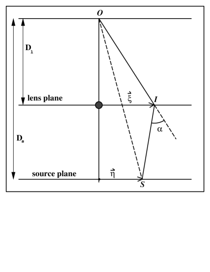
FIG. 1.: The lensing problem in standard gravitational lensing. The point $O$ represents the observer. The point $S$ represents the source. The lens mapping can be interpreted as a map that takes the point $I$ in the lens plane into the point $S$ in the source plane.

FIG. 2.: Diagram of image distortion. The source’s worltube intersects the observer’s past lightcone in a region free of caustics. The source’s visible shape is defined by the intersection. The pencil of rays between the source’s shape and the observer carries the shape of the source into the shape of the image, on the observer’s celestial sphere. The pencil of rays can be described by geodesic deviation vectors (connecting vectors of the observer’s lightcone) from a central null ray connecting the center of the source’s shape to the observer.

FIG. 3.: Vectors associated with the null geodesic that joins the source to the observer. The vector $\ell$ is tangent to the null geodesic. The vectors $(e_{1},e_{2})$ are spacelike, orthogonal to $\ell$, orthonormal and parallel progagated along the geodesics. The vectors $(M_{1},M_{2})$ are linearly independent Jacobi fields which coincide with $(e_{1},e_{2})$ at the location of the source (not shown).

FIG. 4.: The connecting vectors in Schwarzschild spacetime. The vector $M_{1}\equiv\partial/\partial\psi$ lies on the plane defined by the source, the observer and the lens. The vector $M_{2}\equiv\partial/\partial\gamma$ lies on the direction orthogonal to such a plane. The inverse radial distance to the source ($l\equiv(\sqrt{2}r)^{-1}$) is used as a parameter along the null geodesic that connects the source to the observer. The function $\Theta(l,\psi)$ represents the angular location of the source with respect to the lens.

FIG. 5.: Distortion by a Schwarzschild black hole. The inverse ratio of the semiaxes of the image divided by the inverse ratio of the semiaxes of the source is plotted for fixed distance between the source and the deflector, equal to the distance between the lens and the observer, as a function of the image angle. For large image angle the distortion decreases, since the ratio tends to 1 as $\psi\to\pi/2$. For small image angle, the geodesics that arrive at the observer go through a strong gravitational field, and the distortion is large. The distortion is infinite (where the inverse ratio is zero) for the images of sources that lie on the caustics the observer’s lightcone.

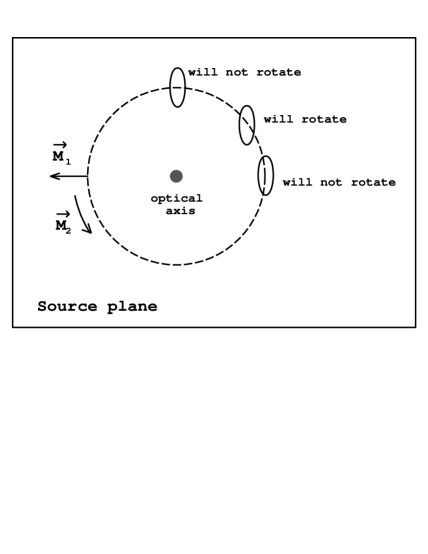
FIG. 6.: Distortion by a Schwarzschild black hole. The axial symmetry in the source plane leads to no orientation distortion if the semiaxes of the elliptical source are aligned with the connecting vectors $M_{1}^{a}$ and $M_{2}^{a}$. $M_{1}^{a}$ points in the polar angular direction, whereas $M_{2}^{a}$ points along the radial direction on the source plane. Thus, only sources aligned with the radial direction experience no distortion of orientation.

REFERENCES

- [1] D. M. Wittman et al., Detection of weak gravitational lensing distortions of distant galaxies by cosmic dark matter at large scales, astro-ph/0003014 v4.
- [2] J. Ehlers, S. Frittelli, and E. T. Newman, Gravitational lensing from a spacetime perspective, contribution to the Festschrift in honor of John Stachel, edited by Juergen Renn, submitted March 1999.
- [3] S. Frittelli and E. T. Newman, Phys. Rev. D. 59, 124001(5) (1999).
- [4] S. Frittelli, T. P. Kling, and E. T. Newman, Phys. Rev. D 61, 064021(14) (2000).
- [5] S. Frittelli, T. P. Kling, and E. T. Newman, Image distortion from optical scalars in non-perturbative gravitational lensing, 2000, preprint.
- [6] A. O. Petters, J. Math. Phys. 34, 3555 (1993).
- [7] A. O. Petters, J. Math. Phys. 38, 1605 (1997).
- [8] R. Penrose, in Perspectives in Geometry and Relativity, edited by B. Hoffmann (Indiana University Press, Bloomington, 1966), p. 259.
- [9] R. Blandford et al, MNRAS 251, 600 (1991)
- [10] V. I. Arnol’d, Mathematical Methods of Classical Mechanics, 2nd ed. (Springer-Verlag, New York, 1978).
- [11] V. I. Arnol’d, S. M. Gusein-Zade, and A. N. Varchenko, Singularities of Differentiable Maps (Birkhäuser, Boston, 1985), Vol. I.
- [12] M. V. Berry, J. Opt. Soc. Amer. A4, 561 (1987).
- [13] M. V. Berry, Extreme twinkling and its opposite, 1997, proceedings of the 15th International Conference on General Relativity and Gravitation, Pune, India.
- [14] R. Penrose and W. Rindler, Spinors and Space-time (Cambridge University Press, Cambridge, 1984), Vol. II.
- [15] P. Schneider, J. Ehlers, and E. E. Falco, Gravitational Lenses (Springer-Verlag, New York, 1992).
- [16] V. Perlick, Ray optics, Fermat’s Principle and Applications to General Relativity, Lecture Notes in Physics m61 (Springer-Verlag, New York, 2000).
- [17] R. D. Blanford and R. Narayan, Ap. J 310, 568 (1986).
- [18] V. Perlick, Gravitational lensing from a geometric viewpoint, in Einstein’s field equations and their physical implications, Springer’s Lecture Notes in Physics No. 540, edited by Bernd Schmidt (Springer, New York, 2000).
- [19] V. Perlick, talk presented at the Gravitational Lensing parallel session of the Ninth Marcel Grossman Meeting, Rome, July 2-8, 2000.
- [20] K. Rauch and R. Blandford, ApJ 421, 46 (1994).
- [21] V. F. Panov and Yu, G. Sbytov, Sov. Phys. JETP 74, 411 (1992).
- [22] T. P. Kling and E. T. Newman, Phys. Rev. D. 59, 124002(5) (1999).
- [23] S. Frittelli, C. N. Kozameh, and E. T. Newman, J. Math. Phys. 36, 4984 (1995).
- [24] S. Frittelli, C. N. Kozameh, and E. T. Newman, J. Math. Phys. 36, 6397 (1995).