From Now to Timelike Infinity on a Finite Grid

Abstract

We use the conformal approach to numerical relativity to evolve hyperboloidal gravitational wave data without any symmetry assumptions. Although our grid is finite in space and time, we cover the whole future of the initial data in our calculation, including future null and future timelike infinity.

I Introduction

In the articles Hu99ht ; Hu99as ; Hu00nc ; HuWXXxx we presented a complete code for solving the conformal Einstein equations which will allow us to study many interesting questions about the global structure of spacetimes by performing numerical experiments. In the present paper we want to demonstrate some of the unique capabilities of this code by a simple example: We calculate the time evolution of gravitational wave data without continuous symmetries. The data are prescribed on a hyperboloidal, whence spacelike, initial slice extending to future null infinity. Starting from this slice, we calculate a conformal spacetime $(M,g_{ab})$ by solving the conformal time evolution equations. On the region $\tilde{M}$ of the conformal spacetime on which the variable $\Omega$, the conformal factor, is positive, the metric $\tilde{g}_{ab}=\Omega^{-2}g_{ab}$ defines an asymptotically flat solution to Einstein’s vacuum field equations. We call $(\tilde{M},\tilde{g}_{ab})$ the physical spacetime. The boundary of $\tilde{M}$ in $M$, given by the set $\{\Omega=0\}$, represents future null infinity, ${\cal J}^{+}$, and future timelike infinity, $i^{+}$.
In our evolution the relevant part of the set $\{\Omega=0\}$ is completely covered by a numerical grid. Therefore, embedding the physical spacetime into a larger conformal spacetime implies that the determination of the gravitational radiation is a well-defined, gauge ambiguity-free procedure and that we avoid any influence of artificial boundaries. It also allows very accurate determination of the fall-off behaviour of physical quantities near the different infinities.
Our data are chosen sufficiently close to Minkowski data, so that the solution admits a regular point $i^{+}$ in the conformal extension. However, they are also far enough away to produce a spacetime which differs significantly from Minkowski space. It has been known theoretically for some time that sufficiently weak data should admit a regular point $i^{+}$ at timelike infinity Fr87ot (cf. also ChK93TG for similar results for weak Cauchy data). However, it is a quite remarkable fact that this point can be modelled in a numerical calculation with the precision discussed below.
In the present paper we shall not attempt to discuss the background of the conformal approach again. We refer the reader to Hu99ht and to the recent survey article by J. Frauendiener Fr00ci . In section II we shall describe the given data. Then we discuss their evolution (section III) and show, in particular, that we have indeed covered the initial hypersurface as well as future null infinity and timelike infinity.

II The initial data

To calculate permissable initial data we use the numerical scheme described in Hu00nc , to which we refer for details. There, on an initial hypersurface we give a boundary defining function $\bar{\Omega}$, which will be related to the conformal factor $\Omega$ and the solution $\phi$ of equation (LABEL:Yamabe) by $\Omega=\bar{\Omega}/\phi$, and a conformal 3-metric $h_{ab}$. The 3-metric is chosen such that the tracefree part of the extrinsic curvature of the surface $\bar{\Omega}=0$, the initial cut ${\cal S}$ of null infinity, must vanish.
Then we solve the Yamabe equation,

where $\,{}^{\scriptscriptstyle(3)\!\!\!\>}\nabla$, $\,{}^{\scriptscriptstyle(3)\!\!\!\>}\Delta$, and $\,{}^{\scriptscriptstyle(3)\!\!\!\>}R$ are the derivative operator, the Laplace operator, and the Ricci scalar associated with $h_{ab}$, and $\tilde{k}$ is a positive constant, which we choose to be $\tilde{k}=3$. The solution $\phi$ of the Yamabe equation, the given free functions $\bar{\Omega}$ and $h_{ab}$, and two more free functions, namely the trace $k$ of the conformal extrinsic curvature of the initial slice and the Ricci scalar $R$ of the conformal spacetime, define a set of data for the conformal field equations. Our choices for the free functions are

(2)

If $\phi$ is a solution of the Yamabe equation with respect to $\bar{\Omega}$ and $h_{ab}$, then for any positive function $\theta$ the solution of the Yamabe equation with respect to $\theta\bar{\Omega}$ and $h_{ab}$ is $\phi\sqrt{\theta}$. Therefore, the calculated data depend on the location of ${\cal S}$ but not on the choice of $\bar{\Omega}$ in the interior, and there is no loss of generality, if we choose $\bar{\Omega}$ to be spherically symmetric. The 3-metric $h_{ab}$ is obtained by perturbing the $\underline{x}\underline{x}$ component away from Minkowski data. The chosen perturbation has no obvious continuous symmetry, but it is reflection symmetric at the planes $x=0$, $y=0$, and $z=0$. For that reason it is sufficient to plot the octant $\{(x,y,z)|x\geq 0,y\geq 0,z\geq 0\}$, although the calculation has been performed for $(x,y,z)\in[-1.25,1.25]\times[-1.25,1.25]\times[-1.25,1.25]$. The choices of $k$ and $R$ are pure gauge. The function $k$ determines the initial time derivative $\Omega_{0}$ of the conformal factor $\Omega$ through the relation (7) of Hu00nc , the choice of $R$ determines the values of certain curvature components $\,{}^{\scriptscriptstyle(1,1)\!\!\!\>}\hat{R}_{ab}$ and $E_{ab}$ and the variable $\omega$, obtained by applying the wave operator applied to $\Omega$. To calculate initial data, we use a spectral bases of $46\times 44\times 44$ elements. The maximum value of the constraint violation on the initial slice is then of order $10^{-4}$. The left graphic in figure 1 shows the metric component $h_{\underline{x}\underline{x}}$ on the $z=0$ plane for a value of $A=1$.

Figure 1: The initial values for the metric component $h_{\underline{x}\underline{x}}$ (left) and the real part of the curvature invariant $\tilde{I}$ (right) on the $z=0$ plane. Only the physical part of the grid is shown.

The plane $z=0$ is the plane, on which the perturbation of $h_{\underline{x}\underline{x}}$ assumes its maximum in the physical region, which is approximately $0.025$. A priori, it is not clear, whether the perturbation is not just a coordinate effect. The right graph in figure 1 shows the real part $\Re(\tilde{I})$ of the curvature invariant

where $\tilde{\psi}_{ABCD}$ is the Weyl spinor of the physical spacetime, $E_{ab}$ the electric part of the rescaled conformal Weyl tensor, $B_{ab}$ its magnetic part, and $i=\sqrt{-1}$. Since this curvature invariant does not vanish, our data do not correspond to Minkowski space. The curvature invariant $\Re(\tilde{I})$ assumes its maximum value of approximately $0.00068$ at the origin. The maximum value for an amplitude $A=2.0$ is approximately $0.00270$. The curvature invariant $\Re(\tilde{I})$ is therefore approximately proportional to $A^{2}$. There is another local maximum at $y\approx 0.55$ with a value of approximately $0.00061$. The physical length of the $y$ coordinate line connecting this maximum with the origin is about $1.25$.

III The time evolution

We split the discussion of the time evolution of our data into three parts. The first part describes the conformal structure of the spacetime. In the second part we describe how we proceed to reconstruct properties of the associated physical spacetime, i. e. the proper time of observers. Issues related to gravitational radiation, such as the longtime decay of the Bondi mass, are dealt with in the third part. To evolve our data, we have to choose five gauge source functions, namely $q=\ln(N/\sqrt{h})$, where $N$ is the lapse and $h$ the determinant of $h_{ab}$, the three components of the shift $N^{a}$, and the Ricci scalar $R$. In our case the simplest choice,

(4)

is sufficient to cover the entire future of the initial data. The size of the next numerical time step is calculated from the Courant-Friedrich-Levy condition at each step as described in Fr98ntb . Corresponding time slices of runs with different resolutions do in general not coincide, since the size of the time step depends on the 3-metric $h_{ab}$, which is a variable of our system. Simultaneous to the time evolution equation we solve 15 ordinary differential equations describing geodesics of the physical metric $\tilde{g}_{ab}$ (cf. HuWXXxx for numerical details). These world lines represent observers in the physical spacetime. Initially the observers are placed at coordinate values of $(0,0,0)$, $(\pm\frac{1}{2},0,0)$, $(0,\pm\frac{1}{2},0)$, $(0,0,\pm\frac{1}{2})$, and $(\frac{\pm 1}{2\sqrt{3}},\frac{\pm 1}{2\sqrt{3}},\frac{\pm 1}{2\sqrt{3}})$. As initial tangent vector we choose the normal of the initial slice and normalise it with respect to the physical metric $\tilde{g}_{ab}$. In addition to the observers in physical spacetime we calculate the orbits of 1986 “Bondi observers moving along generators of null infinity”. Their orbits define a discretisation of $\cal J$ and enable us to calculate radiative quantities (cf. HuWXXxx for details). The Bondi observers are placed at a uniform grid parametrising the initial cut ${\cal S}$ of $\cal J$. They are placed at the north and the south pole and at $64\times 31$ gridpoints covering $(\vartheta,\varphi)\in]0,\pi[\times[0,2\pi[$. An important property of every numerical simulation is an error estimate. The convergence analysis of runs with spatial grids of $(50^{3})$, $(100^{3})$, and $(150^{3})$ gridpoints performed on slices at $t=0.0$, $0.24$, $0.49$, $0.72$, and $0.92$ gives an estimate for the absolute maximal error in any variable of less than $0.001$. This value agrees with the errors obtained when reproducing exact solutions with the same code Hu99as . We have also performed convergence analyses for each plot shown. If not explicitely mentioned, the error estimate of the convergence analysis suggests, that the error is at most of the order of the line thickness in the plots.

III.1 The conformal spacetime

During the evolution of our data we monitor in particular the behaviour of the conformal factor $\Omega$. We will have covered the entire physical future of the initial data, if the region $\{\Omega>0\}$ vanishes for one slice, since the physical spacetime is identical with the set $\{\Omega>0\}$. The orbits of the Bondi observers generate the surface $\{\Omega=0\}$. In figure 2

Figure 2: The projection of representative null generators of $\cal J$ onto the $(z,t)$ plane near the focal point.

we plot their orbits near their focal point. Due to practical reasons we restrict ourselves to the projection onto the plane $\{x=0,y=0\}$ and a representative selection of our 1986 Bondi observers, namely the observers initially placed at the 33 points $(\vartheta,\varphi)=(0,0),(\pi/32,0),\ldots,(\pi,0)$. Plots showing the projections to the planes $\{y=0,z=0\}$ and $\{x=0,z=0\}$ and projections of all the other orbits give corresponding results. It should also be pointed out that the size of a grid cell in the $150^{3}$ run we present is $\Delta t\times\Delta x\times\Delta y\times\Delta z\approx 0.003\times 0.017^{3}$ near the focal point. The generators of $\cal J$ clearly meet within the volume of one grid cell. The result from a $100^{3}$ run is visibly indistinguishable from the $150^{3}$ run, in the $50^{3}$ run the focal point has a slightly smaller $t$ coordinate, namely $\approx 0.996$, which is still in excellent agreement, since the size of the $50^{3}$ grid cells is $\approx 0.009\times 0.05^{3}$ near the focal point, which is larger than the deviation of the runs. We have continued our calculation beyond the focal point up to $t=1.1$ to check regularity of the conformal spacetime at the focal point. Since we have completely covered the physical future of our initial slice at $t=1$ already, it makes no sense to integrate further. Even beyond the focal point the conformal spacetime stays regular. Therefore the focal point is an excellent candidate for a regular $i^{+}$. And indeed, as we will see later, physical observer will reach this point after infinite proper time. Since we have found a complete $\mbox{$\cal J$}{}^{+}$ and a regular $i^{+}$, the constructed spacetime possesses qualitatively the same asymptotic structure as the Minkowski space. Quantitatively, there are differences in the asymptotics as can be seen from figure 3,

Figure 3: Time evolution of real part of conformal curvature invariant $I$ on the positive $y$ axis (only the physical region of conformal spacetime is shown).

where we plot the real part $\Re(I)$ of the conformal curvature invariant

on the physical portion of the grid. The quantity $\psi_{ABCD}$ denotes the rescaled Weyl spinor. There is a significant amount of rescaled conformal curvature at $\mbox{$\cal J$}{}^{+}$ and at $i^{+}$, indicating a non-vanishing fall-off coefficient in the expansion of the corresponding physical curvature invariant $\Re(\tilde{I})$ at infinity.

III.2 Reconstructing the associated physical spacetime

When we reconstruct the physical spacetime from the conformal spacetime, we have to consider two types of quantities. The first type consists of those quantities which can be expressed as a regular expression in the variables of the conformal field equations. Figure 4

Figure 4: Time evolution of the real part of the physical curvature invariant $\tilde{I}$ on the positive $y$ axis.

shows the time evolution of the value of $\Re(\tilde{I})$, which is such a quantity, on the $y$ axis. We see that the time evolution of the two maxima of the initial data is dominated by a rapid decay towards future null and future timelike infinity, although there is another, smaller extremum forming in between the initial maxima. This smaller extremum can best be seen in the contour plot on top of the surface plot. In the contour plot we have also marked the location of $\mbox{$\cal J$}{}^{+}$. With a code performing the numerical integration in physical spacetime we would only be able to calculate figure 4, but not figure 3. Since the physical curvature invariant decays so rapidly to zero (at a conformal time of $0.6$ it has already decayed by a factor of order $10000$), only a very accurate physical code could resolve the fall-off at a large physical time. In the conformal picture the decay has been factored out by choosing the rescaled conformal Weyl tensor as variable. We calculate the conformal invariant $\Re(I)$ and the conformal factor $\Omega$, which do not change dramatically during the whole time evolution, and then get the physical invariant by multiplying the conformal curvature invariant with the appropriate powers of the conformal factor (equations LABEL:PhysCurvInv and LABEL:ConformalCurvInv). A convergence analysis shows that the numerical prediction of the behaviour of $\Re(\tilde{I})$ for a $150^{3}$ calculation is indistinguishable from the $100^{3}$ calculation for the whole calculation up to $i^{+}$. At the last slice of the $100^{3}$ run before $i^{+}$ the curvature invariant has decayed by a factor of more than $10^{20}$. Due to the effect of rounding errors, a physical code working with 8 byte reals could not resolve the decay over such a large range, regardless of the grid size required to achieve the required accuracy. The physical metric $\tilde{g}_{ab}=\Omega^{-2}g_{ab}$ blows up at infinity, since the conformal metric $g_{ab}$ is regular everywhere. The second type of quantity consists of those quantities which describe physical distances. They, of course, must blow up when approaching $i^{+}$ or $\mbox{$\cal J$}{}^{+}$. A typical example is the proper time of observers. We will see in the following paragraphs, that the question “For how long can we numerically calculate the measurements of an observer?” is closely tied to the numerical question “How well can we resolve the neighbourhood of the surface $\{\Omega=0\}$?”. Figure 5

Figure 5: The thin line represents the world line of an observer (timelike physical geodesic) starting at $(x,y,z)=(\frac{1}{2\sqrt{3}},\frac{1}{2\sqrt{3}},\frac{1}{2\sqrt{3}})$ and going to $i^{+}$. The thick line represents $\mbox{$\cal J$}{}^{+}$. The particular behaviour of the world line near $i^{+}$ is due to the particular choice of its initial velocity.

shows the world line of a representative observer, who is initially placed at $(x,y,z)=(\frac{1}{2\sqrt{3}},\frac{1}{2\sqrt{3}},\frac{1}{2\sqrt{3}})$, in an $(r=\sqrt{x^{2}+y^{2}+z^{2}},t)$ plot. The world line runs into $i^{+}$ as expected. We can plot the $x$, $y$, and $z$ coordinates of the world line of the observer as a function of conformal time. If our spacetime were a representation of Minkowski space, and if we were to choose the same gauge source functions, the differences $x-y$, $x-z$, and $y-z$ would vanish for all times, due to symmetry reasons. Figure 6

Figure 6: Oscillation of an observer in coordinate space: The differences $x-y$ (solid), $x-z$ (dashed), and $y-z$ (dotted) as a function of conformal time $t$ which would all be $0$ for Minkowski data ($A=0$).

shows, that this is not the case in the computed spacetime. The observer oscillates around the Minkowski orbit — he is pushed around by the gravitational wave. The amplitude of the oscillation is small compared to the coordinate values. By plotting the difference we make the oscillation visible. A plot of the conformal factor along the world line of our observer gives the left graph of figure 7.

Figure 7: Left: Conformal factor $\Omega$ along an observer world line for the entire time evolution. Right: The same near $i^{+}$ (right) for a $50^{3}$ ($\times$), an $100^{3}$ ($+$), and an $150^{3}$ ($\star$) run.

The right graph of that figure shows the vicinity of $i^{+}$ for the $50^{3}$ ($\times$), the $100^{3}$ ($+$), and the $150^{3}$ ($\star$) runs. Obviously, the finer the resolution the closer we get to the (quadratic) zero of $\Omega$. When calculating the physical geodesics we also calculate the proper time $\tau$ as a function of the conformal time $t$. In Figure 8

Figure 8: Proper time along an observer world line near $i^{+}$ for a $50^{3}$ ($+$), an $100^{3}$ ($\times$), and an $150^{3}$ ($\star$) run.

we show the result for our observer near $i^{+}$. In the $50^{3}$ run we have covered a proper time interval of $[0,300]$, in the $100^{3}$ run an interval of $[0,350]$, and in the $150^{3}$ run an interval of $[0,700]$. When the integration time is measured in units of the (Bondi) mass $m_{B}(0)$ on the initial slice, the last number is more than $600\,000\;m_{B}(0)$. In figure 9

Figure 9: Bondi time of the Bondi observer at the north pole as a function of conformal time.

we plot the Bondi time $u$ of an observer initially placed at the north pole of $\cal J$ for the conformal time interval $[0,1]$. Most conspicuous is the rapid growth near $i^{+}$, with the largest value $u\approx 950$.

III.3 The decay of the Bondi mass

Here we shortly sketch how we calculate the Bondi mass. Details are given in HuWXXxx . The Bondi mass of a cut ${\cal S}_{u}$ of $\cal J$ is given by

$$m_{B}=-\int_{{\cal S}_{u}}\left(\check{\psi}_{2}+\check{\sigma}\dot{\bar{\check{\sigma}}}\right)\;d^{2}{\cal S},$$ (6)

where $\check{\hphantom{g}}$ denotes quantities with respect to a conformal metric $\check{g}_{ab}=\alpha^{-2}g_{ab}$ in which $\cal J$ is expansion free. The quantity $\check{\sigma}$ is one of the spin coefficients in the Newman-Penrose formalism, its Bondi time derivative $\dot{\check{\sigma}}$ is the news function. When calculating the world lines of Bondi observers, we keep track of the evolution of $\alpha$ for each observer and we parallelly transport with respect to $\check{g}_{ab}$ the null frame associated with the observer. Since the $u=\mbox{const}$ cuts do in general not coincide with the $t=\mbox{const}$ cuts, we have to locate the $u=\mbox{const}$ cuts and interpolate onto them from the $t=\mbox{const}$ cuts before we perform the integration. Once the initial value of the Bondi mass $m_{B}(0)$ is determined, there is an alternative calculation of the Bondi mass, using the mass loss formula:

$$m_{B}(u)=m_{B}(0)-\int_{0}^{u}\int_{{\cal S}_{u^{\prime}}}\left(\dot{\check{\sigma}}\dot{\bar{\check{\sigma}}}\;d^{2}{\cal S}\right)\;du^{\prime}.$$ (7)

The latter method usually gives much smaller errors. Hence we use (7) to calculate the time evolution of the Bondi mass. The initial value is taken from the most accurate calculation, namely the $150^{3}$ run. In our setup $\check{\sigma}$ is $0$ on the initial slice. Figure 10

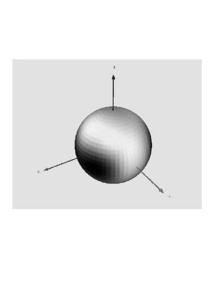
Figure 10: $\psi_{2}$ on the initial cut of $\cal J$. Values range from $-0.148$ (black) to $0.115$ (white).

shows the integrand $\check{\psi}_{2}$ on the initial cut of $\cal J$. Obviously there is a strong high order moment. Since the maximal value of $|\check{\psi}_{2}|$ is about $0.15$, and the initial value of the Bondi mass is about $0.00104$, the high order moments are by a factor of order $100$ stronger than the monopole moment, which is the Bondi mass. Figure 11

Figure 11: Bondi mass as a function of Bondi time.

shows the Bondi mass as a function of the Bondi time $u$ on a logarithmic scale (the abscissa is $\log(u+0.1)$). We observe a rapid decay in a first stage which lasts until $u\approx 0.15$. Then there is a slower decay lasting until $u\approx 1.1$. To see what happens after this stage we change the scale of the ordinate in figure 12,

Figure 12: Bondi mass as a function of Bondi time at late times for $50^{3}$ ($\times$), $100^{3}$ ($+$), and $150^{3}$ ($\star$) runs.

where we plot the Bondi mass against a non-logarithmic time scale. Since the Bondi mass has already decayed by a factor of about $200$, even our small numerical error becomes an issue. The result from the $50^{3}$ (indicated by $\times$) run significantly differs from the results for the $100^{3}$ ($+$) run, whereas the later almost coincides with the results of the $150^{3}$ ($\star$) run. Analytically the Bondi mass of a spacetime with a regular $i^{+}$ must vanish at $i^{+}$. It is not clear, whether the final value of the computed Bondi mass would eventually vanish, if we integrated even longer, or whether this offset is due to a numerical error in the initial value for the Bondi mass, which mainly depends on how accurate the provided initial data solve the constraints.

IV Conclusion

We have calculated the future time evolution of hyperboloidal gravitational wave data, which do not possess any continuous symmetry. We have seen that the conformal approach allows us to cover the entire physical future of these data with a finite grid and to determine the decay of curvature invariants over ranges unreachable by codes working in physical spacetime. Due to the use of higher order methods we can use fairly coarse grids. Since the grids used are coarse, we only need moderate amounts of computer resources, in particular our time evolution on a Origin2000 with R10000 processors requires

• less than 15 minutes on 8 processors for a $50^{3}$ run, where we need 87 time steps to cover $i^{+}$,

• less than 2 hours on 16 processors for a $100^{3}$ run, where we need 173 time steps to cover $i^{+}$, and

• less than 6 hours on 27 processors for a $150^{3}$ run, where we need 263  time steps to cover $i^{+}$.

Already in the $50^{3}$ run the error is at most a few percent. With the $150^{3}$ run we achieve an error of less than one part in thousand.

References

- (1) P. Hübner, Class. Quantum Grav. 16, 2145 (1999).
- (2) P. Hübner, Class. Quantum Grav. 16, 2823 (1999).
- (3) P. Hübner, gr-qc/0010052 pp. 1–22 (2000).
- (4) P. Hübner and M. Weaver, in preparation.
- (5) H. Friedrich, Comm. Math. Phys. 107, 587 (1987).
- (6) D. Christodoulou and S. Klainerman, The Global Nonlinear Stability of the Minkowski Space (Princeton University Press, 1993).
- (7) J. Frauendiener, Liv. Rev. in Relativity (2000).
- (8) J. Frauendiener, Phys. Rev. D 58(6), 064003/1 (1998).