Møller energy of the nonstatic spherically symmetric metrics.

Abstract

The energy distribution in the most general nonstatic spherically symmetric space-time is obtained using Møller’s energy-momentum complex. This result is compared with the energy expression obtained by using the energy-momentum complex of Einstein. Some examples of energy distributions in different prescriptions are discussed.

I Introduction

The absence of a unique way of defining energy and momentum in general relativity has caused much debate. This subject continues to be one of the most active areas of research in general relativity. In spite of many attempts aimed at obtaining an adequate expression for local or quasi-local energy and momentum, there is still no generally accepted definition known. This has resulted in diverse viewpoints on this subject. In a series of papers, Cooperstock [1] hypothesized that in general relativity energy and momentum are located only to the regions of nonvanishing energy-momentum tensor and consequently the gravitational waves are not carriers of energy and momentum. This hypothesis has neither been proved nor disproved. Since the advent of Einstein’s energy-momentum complex, used for calculating energy and momentum in a general relativistic system, many energy-momentum complexes have been found, for instance, Landau and Lifshitz, Papapetrou, and Weinberg (see in [2] and also references therein). The major difficulty with these definitions is that they are coordinate-dependent, with the computations of energy and momentum only giving meaningful results if calculations are carried out in “Cartesian coordinates”. This motivated Møller [3] to construct an expression which enables one to evaluate energy in any coordinate system. However, Møller’s energy-momentum complex suffered some criticism (see [4]).

Over the past two decades a large number of definitions of quasi-local mass (associated with a closed two-surface) have been proposed (see in [5, 6] and references therein). Though Penrose[7] pointed out that a quasi-local mass is conceptually important, a serious problem with the known quasi-local mass definitions is that these do not comply even for the Reissner-Nordström and Kerr space-times[8]. Moreover, the seminal quasi-local mass definition of Penrose is not adequate to handle the Kerr metric[9]. On the contrary, several energy-momentum complexes have been showing a high degree of consistency in giving the same and acceptable energy and momentum distribution for a given space-time. This has been found for many asymptotically flat[10, 11, 12, 13, 14] as well as asymptotically non-flat space-times[15].

Recently Virbhadra[2] investigated whether or not the energy-momentum complexes of Einstein, Landau and Lifshitz, Papapetrou, and Weinberg give the same energy distribution for the most general nonstatic spherically symmetric metric, and to a great surprise he found that these definitions disagree. He noted that the energy-momentum complex of Einstein furnished a consistent result for the Schwarzschild metric whether one calculates in Kerr-Schild Cartesian coordinates or Schwarzschild Cartesian coordinates. The definitions of LL, Papapetrou and Weinberg give the same result as in the Einstein prescription if computations are performed in Kerr-Schild Cartesian coordinates; however, they disagree with the Einstein definition if computations are done in Schwarzschild Cartesian coordinates. Thus, the definitions of LL, Papapetrou and Weinberg do not furnish a consistent result. Based on this and some other investigations, Virbhadra remarked that the Einstein method is the best among all known (including quasi-local mass definitions) for energy distribution in a space-time. Recently in an important paper Lessner[16] argued that the Møller energy-momentum expression is a powerful concept of energy and momentum in general relativity. So in the present paper we wish to revisit the Møller energy-momentum expression and use it to compute the energy distribution in the most general nonstatic spherically symmetric space-time and compare this result with one obtained by Virbhadra in the Einstein prescription. Throughout this paper we use $G=1,c=1$ units and follow the convention that Latin indices take values from $0$ to $3$ and Greek indices take values from $1$ to $3$.

II Virbhadra’s result in the Einstein Prescription

Virbhadra[2] explored the energy distribution in the most general nonstatic spherically symmetric space-time. He used the energy-momentum complex of Einstein. The most general nonstatic spherically symmetric space-time is described by the line element

$$ds^{2}=\alpha(r,t)\,dt^{2}-\beta(r,t)\,dr^{2}-2\gamma(r,t)\,dt\,dr-\sigma(r,t)\,r^{2}\,(d\theta^{2}+\sin^{2}\theta\,d\phi^{2})\text{.}$$ (1)

This has, amongst others, the following well-known space-times as special cases: The Schwarzschild metric, Reissner-Nordström metric, Vaidya metric, Janis-Newman-Winicour metric, Garfinkle-Horowitz-Strominger metric, a general non-static spherically symmetric metric of the Kerr-Schild class (discussed in Virbhadra’s paper[2]).

The Einstein energy-momentum complex is given as

$$\Theta_{i}{}^{k}=\frac{1}{16\pi}H^{\ kl}_{I\ \ ,l},$$ (2)

where

$$H_{i}^{\ kl}=-H_{i}^{\ lk}\ =\ \frac{g_{in}}{\sqrt{-g}}\left[-g\left(g^{kn}g^{lm}-g^{ln}g^{km}\right)\right]_{,m}\ .$$ (3)

$\Theta_{0}^{\ 0}$ and $\Theta_{\alpha}^{\ 0}$ denote for the energy and momentum density components, respectively. (Virbhadra[2] mentioned that though the energy-momentum complex found by Tolman differs in form from the Einstein energy-momentum complex, both are equivalent in import.) The energy-momentum components are expressed by

$$P_{i}=\int\int\int\Theta_{i}^{\ 0}dx^{1}dx^{2}dx^{3}.$$ (4)

Further Gauss’s theorem furnishes

$$P_{i}=\frac{1}{16\pi}\ \int\int\ H_{i}^{\ 0\alpha}\ \mu_{\beta}\ dS\text{,}$$ (5)

where $\mu_{\beta}$ is the outward unit normal vector over the infinitesimal surface element $dS$. $P_{\alpha}$ give momentum components $P_{1},P_{2},P_{3}$ and $P_{0}$ gives the energy.

Virbhadra transformed the line element $(\ref{Genmetric})$ to “Cartesian coordinates” $(t,x,y,z)$ using $x=r\sin\theta\cos\phi,y=r\sin\theta\sin\phi,z=r\cos\theta$ and $t$ remaining the same and then used the Einstein energy-momentum complex to obtain the energy distribution, which is given below.

$$E_{\rm Einst}=\frac{r\left[\alpha\left(\beta-\sigma-r\sigma_{,r}\right)-\gamma\left(r\sigma_{,t}-\gamma\right)\right]}{2\sqrt{\alpha\beta+\gamma^{2}}}.$$ (6)

In the next Section we obtain the energy distribution for the same metric in Møller’s formulation.

III ENERGY DISTRIBUTION IN MØLLER’s FORMULATION

In this Section we first write the energy-momentum complex of Møller and then use this for the most general nonstatic spherically symmetric metric given by the equation $(\ref{Genmetric})$. Note that as the Møller complex is not restricted to the use of “Cartesian coordinates” we perform the computations in $t,r,\theta,\phi$ coordinates, because computations in these coordinates are easier compared to those in $t,x,y,z$ coordinates.

The following is the Møller energy-momentum complex ${\Im}_{I}^{\ k}$ [3] :

$${\Im}_{I}^{\ k}=\frac{1}{8\pi}{\chi}_{I\ \ ,l}^{\ kl}\quad\text{,}$$ (7)

which satisfy the local conservation laws:

$$\frac{\partial{\Im}_{I}^{\ k}}{\partial x^{k}}=0\text{ .}$$ (8)

The antisymmetric superpotential ${\chi}_{I}^{\ kl}$ is

$${\chi}_{I}^{\ kl}=-{\chi}_{I}^{\ lk}=\sqrt{-g}\left[g_{in,m}-g_{im,n}\right]g^{km}g^{nl}\text{ \ .}$$ (9)

${\Im}_{0}^{\ 0}$ is the energy density and ${\Im}_{\alpha}^{\ 0}$ are the momentum density components. Obviously, the energy and momentum components are given by

$$P_{I}=\int\int\int{\Im}_{I}^{\ 0}dx^{1}dx^{2}dx^{3}\text{\ ,}$$ (10)

where $P_{0}$ is the energy while $P_{\alpha}$ denote for the momentum components. Further Gauss’s theorem furnishes the energy $E$ given by

$$E=\frac{1}{8\pi}\int\int{\chi}_{0}^{\ 0\beta}\ \mu_{\beta}\ dS$$ (11)

where $\mu_{\beta}$ is the outward unit normal vector over an infinitesimal surface element $dS$.

For the line element $(\ref{Genmetric})$ under consideration we calculate

$${\chi}_{0}^{\ 01}=\frac{\left(\alpha_{,r}+\gamma_{,t}\right)\sigma r^{2}\sin\theta}{\left(\alpha\beta+\gamma^{2}\right)^{1/2}}\text{\ ,}$$ (12)

which is the only required component of ${\chi}_{I}^{kl}$ for our purpose.

Using the above expression in equation $(\ref{energy})$ we obtain the energy distribution

$$E_{\rm M\o l}=\frac{\left(\alpha_{,r}+\gamma_{,t}\right)\sigma r^{2}}{2\left(\alpha\beta+\gamma^{2}\right)^{1/2}}\text{ \ .}$$ (13)

It is evident that the energy distribution for the most general nonstatic spherically symmetric metric the definitions of Einstein and Møller disagree in general (compare $(\ref{EEinst})$ with $(\ref{EMol})$). However, these furnish the same results for some space-times, for instance, the Schwarzschild and Vaidya space-times[11]. In the next Section we will compute energy distribution in a few space-times using $(\ref{EEinst})$ and $(\ref{EMol})$.

IV
Examples

In this Section we discuss a few examples of space-times in the Einstein as well as the Møller prescriptions.

1. The Schwarzschild solution
   This solution is expressed by the line element

   $$ds^{2}=\left(1-\frac{2M}{r}\right)dt^{2}-\left(1-\frac{2M}{r}\right)^{-1}dr^{2}-r^{2}\left(d\theta+\sin^{2}\theta^{2}d\phi^{2}\right)\text{\ .}$$ (14)

   Equations $(\ref{EEinst})$ and $(\ref{EMol})$ furnish (see also in [3, 13])

   $$E_{\rm Einst}=E_{\rm M\o l}=M$$ (15)

   showing that these two definitions of energy distribution agree for the Schwarzschild space-time.

2. The Reissner-Nordström solution
   The Reissner-Nordström solution is given by

   $$ds^{2}=\left(1-\frac{2M}{r}+\frac{e^{2}}{r^{2}}\right)dt^{2}-\left(1-\frac{2M}{r}+\frac{e^{2}}{r^{2}}\right)^{-1}dr^{2}-r^{2}\left(d\theta^{2}+\sin^{2}\theta d\phi^{2}\right)\text{\ ,}$$ (16)

   and the antisymmetric electromagnetic field tensor

   $$F_{tr}=\frac{e}{r^{2}}\text{\ ,}$$ (17)

   where $M$ and $e$ are respectively the mass and electric charge parameters.

   For this space-time equations $(\ref{EEinst})$ and $(\ref{EMol})$ furnish (see also in [12])

   $$E_{\rm Einst}=M-\frac{e^{2}}{2r}$$ (18)

   and

   $$E_{\rm M\o l}=M-\frac{e^{2}}{r}\text{\ .}$$ (19)

3. The Janis-Newman-Winicour solution
   

   This solution is given by

   $$ds^{2}=\left(1-\frac{B}{r}\right)^{\mu}dt^{2}-\left(1-\frac{B}{r}\right)^{-\mu}dr^{2}-\left(1-\frac{B}{r}\right)^{1-\mu}r^{2}\left(d\theta^{2}+\sin^{2}\theta\ d\phi^{2}\right)$$ (20)

   and the scalar field

   $$\Phi=\frac{q}{B\sqrt{4\pi}}\ln\left(1-\frac{B}{r}\right),$$ (21)

   where

   $$\mu = \frac{2M}{B},$$ (22)

   $$B = 2\sqrt{M^{2}+q^{2}}.$$ (23)

   $M$ and $q$ are the mass and scalar charge parameters respectively. For $q=0$ this solution furnishes the Schwarzschild solution.

   Virbhadra[2] computed the energy expression for this metric using the Eq. $(\ref{EEinst})$. We do the same here using equation $(\ref{EMol})$. Thus we find that

   $$E_{\rm Einst}=E_{\rm M\o l}=M\text{,}$$ (24)

   which exhibits that these two definitions of energy distribution agree for the Janis-Newman-Winicour space-time.

4. Garfinkle-Horowitz-Strominger solution

   The Garfinkle-Horowitz-Strominger static spherically symmetric asymptotically flat solution is described by (see in [17])

   $$ds^{2}=(1-\frac{r_{+}}{r})(1-\frac{r_{-}}{r})^{\nu}dt^{2}-(1-\frac{r_{+}}{r})^{-1}(1-\frac{r_{-}}{r})^{-\nu}dr^{2}-(1-\frac{r_{-}}{r})^{1-\nu}r^{2}(d\theta^{2}+sin^{2}\theta d\phi^{2})\text{\ ,}$$ (25)

   the dilaton field (denoted by $\Phi$) by

   $$exp(2\Phi)=\left(1-\frac{r_{-}}{r}\right)^{\frac{1-\nu}{\lambda}}$$ (26)

   and the antisymmetric electromagnetic field tensor is

   $$F_{ik}=\frac{e}{r^{2}}\text{\ ,}$$ (27)

   where

   $$~{}~{}\nu=\frac{1-{\lambda}^{2}}{1+{\lambda}^{2}}.$$ (28)

   $r_{-}$ and $r_{+}$ are related to mass M and charge e parameters as follows:

   $$M = \frac{r_{+}+\nu r_{-}}{2},$$ (29)

   $$e^{2} = \frac{r_{+}r_{-}}{(1+\lambda^{2})}.$$ (30)

   $\lambda=0$ in this solution gives the Reissner-Nordström solution. Virbhadra[13] proved that for $e=0$ the Garfinkle-Horowitz-Strominger solution reduces to the Janis-Newman-Winicour solution; this fact was not noticed by Garfinkle, Horowitz and Strominger in their paper.

   Chamorro and Virbhadra[14] computed the energy distribution in Garfinkle-Horowitz-Strominger space-time using the energy-momentum complex of Einstein. They found that

   $$E_{\rm Einst}=M-\frac{e^{2}}{2r}\left(1-\lambda^{2}\right)\text{\ .}$$ (31)

   We compute the energy distribution for the Garfinkle-Horowitz-Strominger space-time using equation $(\ref{EMol})$ and obtain

   $$E_{\rm M\o l}=M-\frac{e^{2}}{r}\left(1-\lambda^{2}\right)\text{\ .}$$ (32)

   Thus, these two definitions give different results (there is a difference of a factor $2$ in the second term).

   Now defining

   $${\cal E}_{\rm Einst}:=\frac{E_{\rm Einst}}{M},\quad{\cal E}_{\rm M\o l}:=\frac{E_{\rm M\o l}}{M},\quad{\cal Q}:=\frac{e}{M},\quad{\cal R}:=\frac{r}{M}$$ (33)

   the equations $(\ref{GHSEE})$ and $(\ref{GHSME})$ may be expressed as

   $${\cal E}_{\rm Einst}=1-\frac{{\cal Q}^{2}}{2{\cal R}}\left(1-\lambda^{2}\right)$$ (34)

   and

   $${\cal E}_{\rm M\o l}=1-\frac{{\cal Q}^{2}}{{\cal R}}\left(1-\lambda^{2}\right)$$ (35)

   For $\lambda^{2}=1,{\cal E}_{\rm Einst}={\cal E}_{\rm M\o l}=M$; however, they differ for any other values of $\lambda^{2}$. For any values of $\lambda^{2}<1$, ${\cal E}_{\rm Einst}$ as well as ${\cal E}_{\rm M\o l}$ decrease with an increase in ${\cal Q}^{2}$ and increase with increase in ${\cal R}$. ${\cal E}_{\rm Einst}>{\cal E}_{\rm M\o l}$ and they asymptotically ($\cal R\rightarrow\infty$) reach the value $1$. The situation is just opposite for any values of $\lambda^{2}>1$ : ${\cal E}_{\rm Einst}$ as well as ${\cal E}_{\rm M\o l}$ increase with an increase in ${\cal Q}^{2}$ and decrease with increase in $R$. ${\cal E}_{\rm Einst}<{\cal E}_{\rm M\o l}$ and they asymptotically ($\cal R\rightarrow\infty$) reach the value $1$.

   We plot the energy distributions ${\cal E}_{\rm Einst}$ and ${\cal E}_{\rm M\o l}$ for $\lambda=0$ (Reissner-Nordström space-time) in the figure 1 and for $\lambda^{2}=1.2$ in figure 2.

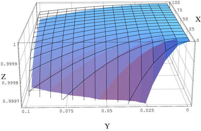
FIG. 1.: ${\cal E}_{\rm Einst}$ and ${\cal E}_{\rm M\o l}$ on Z-axis are plotted against ${\cal R}$ on X-axis and ${\cal Q}$ on Y-axis for ${\lambda}=0$ (Reissner-Nordström metric). The upper (grid-like) and lower surfaces are for ${\cal E}_{\rm Einst}$ and ${\cal E}_{\rm M\o l}$ respectively.

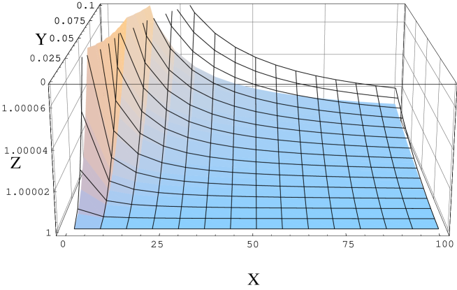
FIG. 2.: ${\cal E}_{\rm Einst}$ and ${\cal E}_{\rm M\o l}$ on Z-axis are plotted against ${\cal R}$ on X-axis and ${\cal Q}$ on Y-axis for ${\lambda^{2}}=1.2$. The upper (grid-like) and lower surfaces are for ${\cal E}_{\rm M\o l}$ and ${\cal E}_{\rm Einst}$ respectively.

V
Conclusion

Based on some analysis of the results known with many prescriptions for energy distribution (including some well-known quasi-local mass definitions) in a given space-time Virbhadra[2] remarked that the formulation by Einstein is still the best one. In a recent paper Lessner[16] argued that the Møller energy-momentum expression is a powerful concept of energy and momentum in general relativity, which motivated us to study this further. We obtained the energy distribution for the most general nonstatic spherically symmetric metric using Møller’s definition. The result we found differs in general from that obtained using the Einstein energy-momentum complex; these agree for the Schwarzschild, Vaidya and Janis-Newman-Winicour space-times, but disagree for the Reissner-Nordström space-time. For the Reissner-Nordström space-time $E_{\rm Einst}=M-e^{2}/(2r)$ (the seminal Penrose quasi-local mass definition also yields the same result agreeing with linear theory[18]) whereas $E_{\rm M\o l}=M-e^{2}/r$. This question must be considered important. Møller’s energy- momentum complex is not constrained to the use of any particular coordinates (unlike the case of the Einstein complex); however it does not furnish expected result for the Reissner-Nordström space-time. We agree with Virbhadra’s remark that the Einstein energy-momentum complex is still the best tool for obtaining energy distribution in a given space-time.

- [1] F. I. Cooperstock, in Topics on Quantum Gravity and Beyond, Essays in honour of L. Witten on his retirement, edited by F. Mansouri and J. J. Scanio (World Scientific, Singapore, 1993); Mod. Phys Lett. A14,1531 (1999).
- [2] K. S. Virbhadra, Phys. Rev. D60, 104041 (1999).
- [3] C. Møller, Annals of Physics (NY) 4, 347 (1958).
- [4] C. Møller, Annals of Physics (NY) 12, 118 (1961); D. Kovacs, Gen. Relativ. Gravit.. 17, 927 (1985); J. Novotny, Gen. Relativ. Gravit.. 19, 1043 (1987).
- [5] J. D. Brown and J. W. York, Jr., Phys. Rev. D47, 1407 (1993).
- [6] S. A. Hayward, Phys. Rev. D49, 831 (1994).
- [7] R. Penrose, Proc. Roy. Soc. London A381, 53 (1982).
- [8] G. Bergqvist,Class. Quantum Gravit. 9, 1753 (1992).
- [9] D. H. Bernstein and K. P. Tod, Phys. Rev. D49, 2808 (1994).
- [10] K. S. Virbhadra, Phys. Rev. D42, 1066 (1990); Mathematics Today 9, 39 (1991); K. S. Virbhadra and J. C. Parikh, Phys. Lett. B317, 312 (1993); Phys. Lett. B331, 302 (1994); K. S. Virbhadra, Pramana - J. Phys. 44, 317 (1995); A. Chamorro and K. S. Virbhadra, Pramana-J. Phys. 45, 181 (1995); J. M. Aguirregabiria, A. Chamorro and K. S. Virbhadra, Gen. Relativ. Gravit. 28, 1393 (1996); S. S. Xulu, Int. J. Theor. Phys. 37, 1773 (1998); Int. J. Mod. Phys. D7, 773 (1998).
- [11] K. S. Virbhadra, Pramana-J. Phys. 38, 31 (1992).
- [12] K. S. Virbhadra, Phys. Rev. D42, 2919 (1990); F. I. Cooperstock and S. A. Richardson, in Proc. 4th Canadian Conf. on General Relativity and Relativistic Astrophysics (World Scientific, Singapore, 1991).
- [13] K. S. Virbhadra, Int. J. Mod. Phys. A12, 4831 (1997).
- [14] A. Chamorro and K. S. Virbhadra, Int. J. Mod. Phys. D5, 251 (1996).
- [15] N. Rosen and K. S. Virbhadra, Gen. Relativ. Gravit. 25, 429 (1993); K. S. Virbhadra, Pramana - J. Phys. 45, 215 (1995); S. S. Xulu,Int. J. Mod. Phys. A (in press), gr-qc/9902022; Int. J. Theor. Phys. (in press), gr-qc/9910015.
- [16] G. Lessner, Gen. Relativ. Gravit. 28, 527 (1996).
- [17] J. H. Horne and G. T. Horowitz, Phys. Rev. D46, 1340 (1992).
- [18] K. P. Tod, Proceedings of Royal Society of London A388, 467 (1983).