A Tolman-Bondi-Lemaitre Cell-Model for the Universe and Gravitational Collapse

Abstract

A piecewise Tolman-Bondi-Lemaitre (TBL) cell-model for the universe incorporating local collapsing and expanding inhomogeneities is presented here. The cell-model is made up of TBL underdense and overdense spherical regions surrounded by an intermediate region of TBL shells embedded in an expanding universe. The cell-model generalizes the Friedmann as well as Einstein-Straus swiss-cheese models and presents a number of advantages over other models, and in particular the time evolution of the cosmological inhomogeneities is now incorporated within the scheme. Important problem of gravitational collapse of a massive dust cloud, such as a cluster of galaxies or even a massive star, in such a cosmological background is examined. It is shown that the collapsing local inhomogeneities in an expanding universe could result in either a black hole, or a naked singularity, depending on the nature of the set of initial data which consists of the matter distribution and the velocities of the collapsing shells in the cloud at the initial epoch from which the collapse commences.

1 Introduction

The conventional cosmological scenarios are based on the Friedmann- Robertson-Walker (FRW) solutions of the Einstein equations. These models have the advantage of being simple, because the universe has been assumed to be isotropic and homogeneous on large enough scales of the order of 300 Mpc and higher. It is thus possible to use these models for making a number of predictions on the large scale structure and evolution of the universe. The disadvantage, however, is that one is no longer able to take into account in an exact manner the various observed inhomogeneities present in the universe, such as the development and evolution of structures such as voids, or local collapsing inhomogeneities such as a gravitationally collapsing massive cloud in a cosmological background, which may represent a sufficiently isolated collapsing massive star which has exhausted its nuclear fuel, or a star cluster, or even a cluster of galaxies evolving dynamically.

The important unsolved problem is thus that of taking into account and modeling the various inhomogeneities, and their evolution in the real universe. We propose here an idealized cell-model for the universe which attempts this task. The universe is no longer assumed to be made up of a uniform and homogeneous matter continuum, but is taken to be consisting of various elementary building blocks embedded in a uniform background. In fact, a complete solution of Einstein equations for a matter continuum consisting of inhomogeneous dust is available, as given by the so called Tolman-Bondi-Lemaitre (TBL) models [1]. The FRW models form a special class of this more general class of models. Using earlier work of Chamorro [2], and Bonnor and Chamorro [3], it is then shown how a model for the evolution of the inhomogeneities in the universe can now be constructed. One of the advantages over former swiss-cheese models is that our picture allows a much richer and diverse structure of the universe as different structures may exist within other structures, all of them ultimately embedded in an otherwise expanding universe. The universe not only has inhomogeneities, but these inhomogeneities may not be uniform in structure. The model presented here, besides generalizing previous swiss-cheese models, makes an attempt to incorporate the inhomogeneities suitably.

We then turn our attention to the problem of gravitational collapse of a massive cloud in such a cosmological background. The gravitational collapse scenarios involving the collapse of a compact body have been explored in quite some detail in recent years, particularly in the context of the cosmic censorship hypothesis (see e.g. Joshi [4], and references there in). The scenario that has been developing from these studies is that for various forms of matter such as dust, perfect fluids, radiation collapse etc. both black holes and naked singularities develop as the end state of collapse depending on the nature of the initial data from which the collapse commences. In fact, it turns out that sets of initial data of matter configurations, in terms of densities and velocity profiles prescribed at the onset of collapse, may yield evolutions within the context of general relativity which would lead to either a black hole or a naked singularity, independently of the form of matter or the equation of state used.

Most of these models have so far been analyzed within an asymptotically flat background, which is best suited for phenomena involving isolated bodies. However, in widely accepted cosmological models describing the present scenario of the expanding universe, spacetime curvatures are non-vanishing throughout the universe, and therefore such a picture of collapse could not be taken to represent a real gravitational collapse of cosmic relevance. On the other hand, considerations of a collapsing inhomogeneity in an expanding universe would represent a more realistic physical situation. It is therefore of interest to study the nature of gravitational collapse in such expanding environments. That way one could find out if the introduction of a cosmological background could possibly affect the nature and outcome of the collapsing local inhomogeneity. Our consideration here show however that the incorporation of a cosmological background does not change the earlier conclusions on gravitational collapse qualitatively. That is, depending on the nature of initial data which consists of the density distribution and velocity profiles of the collapsing shells in the cloud, both black holes and naked singularities would arise.

The plan of the paper is as follows. In Section 2 the cell-model for the universe is constructed, describing its basic building blocks which will account for the elementary inhomogeneities. In Section 3, we consider the gravitational collapse problem in such a cosmological background. Section 4 examines the issue of global visibility of such singularities for faraway observers in the universe. In the concluding Section 5 we discuss the overall scenario and conclusions, and the possibilities of generalizing these results further.

2 A Tolman-Bondi-Lemaitre cell-model for the universe

In line with current ideas about the cell structure of the universe we construct here a model for the universe made up of TBL, and in particular, Friedmann underdense and overdense spherical regions surrounded by compensating thick TBL shells. As we shall see, ultimately all inhomogeneities will be embedded in an expanding Friedmann background of either positive, zero or negative spatial curvature. In construction of such a cell-model we follow and extend ideas contained in Chamorro [2], where models of voids in elliptic Friedmann universe were presented.

Throughout the paper we use Einstein field equations $G_{ab}=-kT_{ab}$ with vanishing cosmological constant, and the cosmic fluid is taken as the dust matter with the stress-energy tensor given by $T_{ab}=\rho u_{a}u_{b}$. All elementary inhomogeneities would be assumed to be spherically symmetric. The field equations for dust matter have already been solved and the solution is the TBL metric given by

$$ds^{2}=-dt^{2}+{{R^{\prime 2}}\over{1+f}}dr^{2}+R^{2}d\Omega^{2},$$ (1)

$$\rho={F^{\prime}\over R^{2}R^{\prime}},\quad\dot{R}^{2}=f+{F\over R}$$ (2)

Here $f(r)$ and $F(r)$ are arbitrary functions of $r$ only, and are interpreted as the energy and mass functions. The energy density is $\rho$, while (.) and (^′) denote partial differentiation with respect to $t$ and $r$.

Figure 1:

Before discussing the basic building blocks of the cell-model in detail, which consist of various types of local inhomogeneities, let us first consider how a single inhomogeneity is inserted in our cell-model in general. The local inhomogeneity (see Fig. 1) is described by a TBL underdense or overdense region F1 (as the case may be ) and is surrounded by a compensating region T of a thick TBL shell which in turn is embedded in the background cosmology of region F2. The metric and the density functions in the three regions are given as

$$ds^{2}=-dt^{2}+{{R_{1}^{\prime 2}}\over{1+f_{1}}}dr^{2}+R_{1}^{2}d\Omega^{2},\quad r<b,\quad\rho_{1}={F_{1}^{\prime}\over R_{1}^{2}R_{1}^{\prime}}$$ (3)

$$ds^{2}=-dt^{2}+{{R^{\prime 2}}\over{1+f}}dr^{2}+R^{2}d\Omega^{2},\quad b<r<c,\quad\rho={F^{\prime}\over R^{2}R^{\prime}}$$ (4)

$$ds^{2}=-dt^{2}+{{R_{2}^{\prime 2}}\over{1+f_{2}}}dr^{2}+R_{2}^{2}d\Omega^{2},\quad c<r,\quad\rho_{2}={F_{2}^{\prime}\over R_{2}^{2}R_{2}^{\prime}}$$ (5)

The solution of Einstein equations in region F1 is given as,

$$R_{1}={F_{1}\over-2f_{1}}(1-\cos u),\quad t-a_{1}(r)=k_{1}(u-\sin u),\quad r<b$$ (6)

where $k_{1}$ is given by,

$$k_{1}={F_{1}\over 2(-f_{1})^{3/2}}$$ (7)

For the region F1 we have $f(r)<0$, $r\geq 0,0\leq\theta\leq\pi,0\leq\phi\leq 2\pi$ and $0<u<2\pi$, $t>a(r)$.

Note that the shell labeled by $r$ is initially singular at $t=a(r)$ for $u=0$(big bang), and since region F1 is elliptic (i.e. $f<0$) in case it is collapsing later on it also becomes singular in the future at the time,

$$t=t_{s}(r)=a(r)+{\pi F\over(-f)^{3/2}}.$$ (8)

For the regions T and F2, depending upon whether the region is elliptic, parabolic or hyperbolic (i.e. $f(r)<0,=0,>0$), the solutions have the following form,

$$R_{i}=-{F_{i}\over 2f_{i}}(1-\cos{\it v}),\quad t-a_{i}(r)={F_{i}\over 2(-f_{i})^{3/2}}({\it v}-\sin{\it v})\;for\;f<0$$ (9)

$$R_{i}={\bigg{(}}{9F_{i}\over 4}{\bigg{)}}^{1/3}[t-a_{i}(r)]^{2/3}\;for\;f=0$$ (10)

$$R_{i}=-{F_{i}\over 2f_{i}}(1-\cosh{\it v}),\quad t-a_{i}(r)=-{F_{i}\over 2f_{i}^{3/2}}({\it v}-\sinh{\it v})\;for\;f>0.$$ (11)

In the elliptic region ${\it v}$ takes values from $0$ to $2\pi$, while in the hyperbolic region it takes values from $0$ to $\infty$. For the intermediate region T we would use the notation $(R_{i}\equiv R,F_{i}\equiv F,f_{i}\equiv f,a_{i}\equiv a,{\it v}\equiv w)$ while for the cosmological background region F2 it shall be $(R\equiv R_{2},F\equiv F_{2},f\equiv f_{2},a_{i}\equiv a,{\it v}\equiv v)$

If the spacetime as described in Fig 1 is to be considered a solution of the field equations, the solution must satisfy the boundary conditions at $r=b$ and $r=c$. The Darmois matching conditions at the boundaries $r=b$ and $r=c$ (see Bonnor & Vickers 1981[5]) require

$$F_{1}(b)=F(b),\quad f_{1}(b)=f(b)$$

$$F_{2}(c)=F(c),\quad f_{2}(c)=f(c)$$

$$R(b,t)=R_{1}(b,t),\quad R_{2}(c,t)=R(c,t)$$ (12)

Thus the above conditions determine the boundary values of the mass and energy functions $(F,f)$ of the intermediate region T for a given inner region F1 and outer cosmological region F2. Note however that there may be discontinuities in the densities across the shells $r=b,c$, as continuity of the functions $F^{\prime},f^{\prime}$ and $R^{\prime}$ is not required by (12).

The ratio of the average density of the region F1, which is $\rho_{1}$, to the exterior Friedmann universe $\rho_{2}$, is given for elliptic universe by

$${\rho_{1}\over\rho_{2}}={\gamma[v(c))]\over\gamma[u(b)]}\left({t-a_{1}(b)\over t-a_{2}(c)}\right)^{2},$$ (13)

$$\gamma(v)={(1-\cos v)^{3}\over(v-\sin v)^{2}},$$ (14)

and for the hyperbolic case it is given by,

$${\rho_{1}\over\rho_{2}}=-{F(c)^{2}\over F(b)^{2}}{f(b)^{3}\over f(c)^{3}}{[\cosh v(c)-1]^{3}\over[1-\cos u(b)]^{3}},$$ (15)

where as in the parabolic case it is,

$${\rho_{1}\over\rho_{2}}=-{18f(b)^{3}\over F(b)^{2}}{[t-a_{2}(c)]^{2}\over[1-\cos u(b)]^{3}}.$$ (16)

Note that if the outer Friedmann region is parabolic or hyperbolic then in the region T we need to have a transition from $f<0$ to $f\geq 0$. This can be achieved smoothly in the TBL model provided $f(r)$ and $F(r)$ be at least $C^{2}$ functions. This is because though we write the solution in three different regions in three different ways it is actually a one continuous function as all the functions and derivatives from either side of $f=0$ match at the transition point, i.e. $f=0$ [6]. An equally important aspect of the solution, if the inhomogeneity is to be inserted smoothly through the intermediate region to the outside cosmological region F2, is that there be no shell-crossings. To avoid shell-crossings we must require for the mass function $F(r)$, $f(r)$ and the singularity time $a(r)$ to satisfy Hellaby and Lake’s conditions as given in Table I of [7].

We discuss now in detail the building blocks or elementary inhomogeneities of the model. For the sake of clarity we would first consider these inhomogeneities in various situations in an outside elliptic exterior (i.e. $f_{2}(r)<0$).

2.1 Expanding void in expanding exterior :

The solutions for the metric (1) corresponding to the regions shown in figure 1 are,

In region F1,

$$R_{1}=k_{1}r(1-cosu),\quad t+\epsilon=k_{1}(u-sinu)$$ (17)

$r<b$, $u<\pi$.

In region T,

$$R=F(-2f)^{-1}(1-cosw),\quad(w-sinw)=2(-f)^{3/2}F^{-1}(t-a)$$ (18)

$b<r<c$, $w<\pi$ .

In region F2,

$$R_{2}=k_{2}r(1-cosv),\quad t=k_{1}(v-sinv)$$

and $r>c$, $v<\pi$.

The inequalities for the angular parameters $u,v$ and $w$ at the present time $t=t_{0}$ are needed to ensure expansion in the three regions. The Darmois matching conditions are enforced at $r=b$ and $r=c$ . In this case a non-simultaneous big-bang (NSBB) is required if the ratio $\rho_{1}/\rho_{2}$ is to be less than 0.6 (see for details Chamorro [2]).

2.2 Expanding void in contracting exterior :

As in the previous case, but now $v>\pi$ at $t_{0}$. Then $v>\pi>u$, and since $d\gamma/dv<0$ one has ${\gamma[v]\over\gamma[u]}<1$; that according to (13) makes it possible to have $\rho_{1}/\rho_{2}<1$ taking suitable values for $a_{1}(b)$ and $a_{2}(c)$. Then by using the Hellaby and Lake conditions for no shell-crossings, it can be seen (as in reference [2]) that the avoidance of these singularities requires having $R^{\prime}<0$ in some region of T. The general appearance of the profiles of the functions $-f$, $F/2k_{1}b$ and $a$ versus $r$ in the intermediate TBL zone ($b,c$) may be the same as that of Fig. 2 in the same reference. However, there is no need of a NSBB to get $\rho_{1}/\rho_{2}$ as small as wanted, provided we choose the ratio $k_{1}/k_{2}$ large enough. Therefore, one can also set $a(r)=0$ to have a simultaneous big bang (SBB) for this building block.

2.3 Contracting overdense region in expanding exterior:

In this instance one needs $u(t_{o})>\pi>v(t_{o})$, that leads to $\rho_{1}/\rho_{2}>1$ for all t and SBB by just taking $k_{1}$ conveniently smaller than $k_{2}$. The intermediate zone T may be described by choosing a function $p(r)\geq 0$ for $r\epsilon(b,c)$ large enough and setting $F^{\prime}/F=3f^{\prime}/2f+p(r)$ to have $F^{\prime}\geq 0$, that together with $a^{\prime}=0$ (SBB in T) leads to $R^{\prime}>0$ and no shell-crossings (see ref. [2]).

2.4 Summary of the former and the other possible building blocks :

There are a total of eight elementary inhomogeneities corresponding to the following characteristics :

1.	$\rho_{1}/\rho_{2}<1$	F1:expansion, F2: expansion	SBB: $k_{1}>k_{2}$, NSBB: $k_{1}\stackrel{{\scriptstyle{>}}}{{<}}k_{2}$
2.	$\rho_{1}/\rho_{2}<1$	F1:expansion, F2:contraction	SBB: $k_{1}>k_{2}$, NSBB: not required
3.	$\rho_{1}/\rho_{2}>1$	F1:contraction, F2:expansion	SBB : $k_{1}<k_{2}$.
4.	$\rho_{1}/\rho_{2}>1$	F1:expansion, F2:expansion	SBB : $k_{1}<k_{2}$, $a_{1}=0$, $a_{2}>0$
5.	$\rho_{1}/\rho_{2}<1$	F1:contraction, F2:expansion	Required NSBB: $a>0$; profiles for f, F and $a$ as in case 1 for no shell-crossings nor surface layers.
6.	$\rho_{1}/\rho_{2}<1$	F1:contraction, F2:contraction	Essentially reducible to cases 3 or 5 as the outermost F-background must be expanding.
7.	$\rho_{1}/\rho_{2}>1$	F1:expansion, F2:contraction	Requires NSBB, but essentially reduces to cases 3 or 5 for same reason as in case 6
8.	$\rho_{1}/\rho_{2}>1$	F1:contraction, F2:contraction	Essentially reduces to cases 3 or 5 again, depending on whether $\rho_{2}/\rho_{0}\geq 1$. $\rho_{0}$ is the density of the outermost F-background.

2.5 Final considerations:

The Darmois matching conditions together with Einstein equations yield that $1/2F(c)$ can be interpreted as the active gravitational mass within the shell of radius $r=c$. That happens to coincide with the mass function introduced by Cahill and McVittie [8]. Thus one might construct a cell-like dust model for the universe by inserting elementary inhomogeneities of the kind considered above in an expanding Friedmann background as depicted in Figure 2. The following interesting features of the model should be noticed :

Figure 2: F is the outermost expanding Friedmann background. F1, F2,…. stand for the voids and overdense regions, expanding or contracting. They are surrounded by their corresponding compensating TBL zones.

a) It allows to put inhomogeneities such as F5 within other inhomogeneities (when the inhomogeneities contain homogeneous and isotropic parts) in contradistinction to the traditional swiss-cheese models $`$a la Einstein-Strauss.

b) The geometrical center of each inhomogeneity may be taken as its center of mass. All such centers may be viewed as fundamental particles of the cosmic fluid, moving exactly as if they were particles of the exterior F-background within which all the inhomogeneities are embedded.

c) Thus the overall average expansion of this model would be described by the dynamics of the exterior Friedmann background.

d) This provides a cell model for the expanding universe where the average problem of Einstein equation: $G_{\mu\nu}(<g>)\neq-<T_{\mu\nu}>$, finds a simple solution.

Though we have discussed here the case of positive curvature Friedmann universe, the results can be easily generalized to the case when the outside Friedmann universe is of zero or negative curvature. In these cases, if $f_{1}(r)<0$, the intermediate TBL region has to take us from positive curvature to zero or negative curvature. As it was mentioned above this is possible because though we write the TBL solution for the three cases in three different forms, it is actually a one continuous solution if the change over is smooth. That is, it is enough that the energy and mass functions in T be $C^{2}$ for the solutions of the Einstein equations to exist. The case $f(r)\geq 0$ can be dealt with without the incommodity of shell-crossings by taking negative curvature solutions for part or all of Region T and for F2.

3 Gravitational Collapse and Singularity Formation

The occurrence of a physical phenomena, as predicted by the theory, is possible only if the conditions assumed under which the proposed models are derived are physically realistic, and are realized in nature. In this context, since the universe is widely believed to be described by an expanding cosmological model at its present stage, it is quite natural to ask whether all the conclusions drawn from consideration of collapse scenarios of isolated bodies in an asymptotically flat background would hold if the cosmological background is taken into consideration. That is, whether a collapsing massive cloud in an expanding universe would give rise to the same conclusions regarding black holes or naked singularities formation. We therefore investigate this issue here with the aim of examining the possible formation of a naked singularity, or a black hole, during the collapse of a dense body in an otherwise cosmological background, to see whether the background imposes any constraints on the occurence of these phenomena.

In fact, it is known that a massive star in the universe does not have sharp boundaries. The star or the compact body has a core which is superdense and an outer layer and crust which is less dense, which is further surrounded by a cloud of much lower density. In a realistic collapse situation, there is always a strong possibility that the core of the star, being superdense and massive, may undergo a continued collapse, while the outer layers of the star may be blown up far away. Thus, in real situations, the core of the star would be collapsing while there would be an intermediate region consisting of a much less dense cloud which could be expanding in a smeared-out expanding universe. Certainly, such considerations apply even more effectively in the case of possible collapse of very large aggregations of matter in the universe, such as a supercluster of galaxies or the great attractor. The cell-model of the universe described in the earlier section thus becomes quite relevant to a real physical scenario.

In the context of gravitational collapse, spherical dust clouds in general relativity have been studied quite extensively [9]. The prescription of matter as pressureless dust could perhaps be regarded as somewhat idealized. However, some authors have considered dust as a good approximation of the form of the matter in the final stages of collapse (see e.g. Penrose [10]). In any case, the study of dust models has led not only to important new advances and insights into various aspects of the gravitational collapse theory, but have also laid the foundation of black hole physics. We therefore consider here the problem of a superdense region of dust in an expanding Friedmann model, and see if the formation of a naked singularity or a black hole would occur as it did in asymptotically flat exteriors.

We shall use here the cell-model formerly described and contemplate the situation of an overdense collapsing region surrounded by an underdense intermediate region, in the exterior background of an expanding Friedmann universe.

The basic idea, in order to examine the existence or otherwise of naked singularities forming as end state of gravitational collapse, is to investigate the structure of families of non-spacelike geodesics of the spacetime to find if there are such families which terminate in the past at the singularity, and in future they are outgoing, reaching a faraway observer. If there are no such families the collapse ends in a black hole, otherwise we have a naked singularity in the spacetime. While outgoing families of non-spacelike geodesics can be treated in general, it is enough for the present purpose to examine outgoing null geodesics radiating away from the singularity. Using the notation,

$$X={R\over r^{\alpha}},\quad\Lambda={F\over r^{\alpha}}$$ (19)

the equation for radial null geodesics can be written as,

$${dR\over d(r^{\alpha})}=\left[1-\sqrt{{f+{\Lambda\over X}}\over 1+f}\right]{R^{\prime}\over\alpha r^{\alpha-1}}\equiv U(X,r^{\alpha}).$$ (20)

We use $r^{\alpha}$ instead of r for convenience in order to examine the structure of the singularity. The exact value of the constant $\alpha\geq 1$ depends on the different initial density and velocity distributions for the collapsing cloud. We first examine the geodesic equation in Region I in order to understand the nature of the singularity which occurs during the collapse of this overdense region. The outgoing null trajectories, if any, then can be traced into Region T and finally to the expanding Region F2. The point $r^{\alpha}=0,R=0$ is a singularity of the above differential equation in Region I. In order to understand the nature of outgoing families, it is necessary to examine the nature of this singularity.

If future directed null geodesics do terminate in the past at the singularity $R=0,r^{\alpha}=0$ with a definite tangent, this is determined by the limiting value of $X=R/r^{\alpha}$ at $R=0,r^{\alpha}=0$. In such a case,

$$X_{0}=\lim_{R\to 0,r^{\alpha}\to 0}{R\over r^{\alpha}}=\lim_{R\to 0,r^{\alpha}\to 0}{dR\over d(r^{\alpha})}=\lim_{R\to 0,r^{\alpha}\to 0}U=U(X_{0},0).$$ (21)

If a real positive value of $X_{0}$ satisfies the above equation, then the singularity could be naked. The above equation has been analyzed in detail. It turns out that the necessary and sufficient condition for the central shell-focusing singularity to be naked, at least locally, is that equation (21) admits a real, positive root $X=X_{0}$. In fact, for the case of TBL models, it is possible to write this equation explicitly as an algebraic equation in terms of the basic initial data parameters $F$ and $f$ [11], and it follows that the central singularity, occurring at the time $t=t_{s}(0)$ where $t_{s}(r)$ denotes the future singularity curve $R(t,r)=0$, is naked under quite general conditions which essentially depend on the behavior of $F$ and $f$ near the center. In particular, for the case when

$$\rho^{\prime}(0)\neq 0,\Theta(0)>0$$ (22)

where $\Theta(r)=r{t_{s}}^{\prime}(r)\sqrt{h(r)}/r^{3(\alpha-1)/2}$, the central singularity is locally naked. When $\rho^{\prime}(0)=0$, a similar condition can be given in terms of $\rho^{{}^{\prime\prime}}(0)$. In all these cases, the global nakedness depends on the global behavior of the functions $F$ and $f$ away from $r=0$. We discuss this issue in the next section.

We note that for the local nakedness of the singularity, the behavior of the functions (subject to $C^{2}$ differentiability) is allowed to be completely arbitrary for $r>0$. Thus for collapse in a cosmological background, that is, for a collapsing region I, that need not be necessarily homogeneous, the behavior of $F_{1}$ and $f_{1}$ at its boundary is not restricted by the local nakedness condition.

So, for a given set of density and velocity profiles, if the collapse produces a naked singularity, then a suitable intermediate region T with the inner boundary at $r=r_{1}$ can exist such that outgoing null geodesics would cross that boundary and might finally escape to a distant external observer.

4 Global Visibility of Singularities

Amongst the various versions of cosmic censorship available in the literature, the strong cosmic censorship hypothesis does not allow the singularities to be even locally naked. The spacetime must then be globally hyperbolic. Hence the case of the existence of a real positive root to equation (21) is a counter-example to the strong cosmic censorship conjecture [11]. However, one may take the view that the singularities which are only locally naked may not be of much observational significance as they would not be visible to observers faraway in the universe, and as such the spacetime outside the collapsing object may be asymptotically predictable. On the other hand, globally naked singularities could have observational significance, as they are visible to an outside observer faraway in spacetime. Thus, one may formulate a weaker version of censorship, whereby one allows the singularities to be locally naked but rules out global nakedness. We examine now this issue of local versus global visibility of the singularity for the models with cosmological background we have been considering. That will provide insight concerning the possibility of global visibility when we vary the initial data, as given by the initial velocity distributions of the cloud.

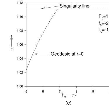
Figure 3: The structure of singularity in the closed ($f<0$) universe case. For the inner TBL collapsing core we take $f(r)=f_{0}r^{2}+f_{m}r^{4}$ and $F=F_{0}r^{3}$. In the cosmological region $f=-r^{2}$ and $F=F_{0}r^{3}$. Here $f_{0}=-2$ and $F_{0}=1$, so the central singularity forms at $t=t_{0}(0)=1.1$. (a) $f_{m}=4$ case. The event horizon meets the center $r=0$ below the singularity and no null trajectories escape to a distant observer. The singularity is only locally naked.(b) $f_{m}=8$. The singularity is globally naked. There is a family of null geodesics from the singularity which meet the boundary of cloud with $R>-F(c)/f(c)$. (c) Graph showing transition from local nakedness to global nakedness, by varying $f_{m}$.

It is shown below that both locally and globally visible singularities, are possible within the scenario we have considered here, depending on the initial conditions. By varying suitable parameters in the regular initial data, we examine the effect on the global visibility of the singularity. Here we study the case of an elliptic universe. We take $a=0,F_{1}=F_{2}=r^{3},f_{2}=-r^{2}$, and $f_{1}=-2r^{2}+f_{m}r^{4}$ with $f_{m}$ such that $f_{1}<0$ within Region I, and we can, in this case, match the inner TBL model (Region I, which consists of a collapsing core and an outer expanding region at the initial epoch) directly with the outside Friedmann model (Region F2) by satisfying the Darmois matching conditions at the boundary $r=c$, which implies,

$$c=\sqrt{1/f_{m}}$$ (23)

We also need that $c<1$, i.e. $f_{m}>1$. We shall say that the singularity is globally visible if the null geodesics coming out of the singularity meet the $r=c$ shell before it starts recollapsing. As we vary the parameter $f_{m}$, we see a transition from a locally naked to a globally naked singularity at $f_{m}=6.75$. Examples of naked singularities which are only locally naked, as well as those of globally naked singularity in a cosmological background, and of the transition, are illustrated in Figure 3.

5 Concluding Remarks

The issue of the end state of gravitational collapse in physically reasonable configurations is most crucial to the cosmic censorship hypothesis. In this context, the present work shows that gravitational collapse of local inhomogeneities in an otherwise expanding universe can give rise to naked (locally or globally) or covered singularities, depending on the initial data of the matter cloud. These conclusions are in line with the earlier conclusions on collapse of a star against an asymptotically flat background. It thus appears that singularities, both naked or covered, are in a way natural to general relativity.

Our work here shows that naked singularities, or black holes, do occur as the end stage of collapse in a cosmological background, where the curvatures are non-vanishing throughout the universe. It follows that the assumption of asymptotic flatness is not crucial to the formation of a covered or naked singularity (see also [12] for an example in Vaidya background). Considerable amount of work has been done in black hole physics, however black hole physics is heavily dependent on the existence of asymptotic flatness, which in fact is not the situation in the large scale physical universe. Thus, questions arise such as wether or not some of the results of black hole physics would be different if considered in a cosmological background. The answer to these questions is certainly important as it would bring black hole physics closer to physical reality, and thus brighten the chances of obtaining its observable features in our universe.

We acknowledge the support from University of Basque Country Grants UPV122.310-EB150/98, UPV172.310-G02/99 and the Spanish Ministry Grant PB96-0250.

References

- [1] R. C. Tolman, Proc. Natl. Acad. Sci. USA (1934), 410; H. Bondi, Mon. Not. Astron. Soc. (1947), 343; G. Lemaître, Ann. Soc. Sci.Bruxelles I, A53, 51(1933).
- [2] A. Chamorro Ap. J, , 51(1991).
- [3] W. B. Bonnor and A. Chamorro, Ap. J, , 461(1991).
- [4] P. S. Joshi, Global Aspects in Gravitation and Cosmology (Clarendon Press, Oxford, 1993).
- [5] W. B. Bonnor and P. A. Vickers, Gen Rel. Grav., ,29(1981).
- [6] R. P. A. C. Newman, Class. Quantum Grav. , 527(1986).
- [7] C. Hellaby and K. Lake, Ap. J,,381(1985).
- [8] M. E. Cahill and G. C. McVitte, J. Math. Phys. 11, 1382(1970)
- [9] D. M. Eardly and L. Smarr, Phys. Rev.D 19, 2239 (1979); D. Christodoulou, Commun. Math. Phys. , 171 (1984); P. S. Joshi and I. H. Dwivedi, Phys Rev D 47, 5357 (1993).
- [10] R. Penrose, in Gravitational Radiation and Gravitational Collapse, Proceedings of the IAU Symposium, edited by C. DeWitt-Morette, IAU Symposium No.64(Reidel,Dordrecht, 1974).
- [11] S. Jhingan and P. S. Joshi, Ann. Israel Phys. Soc., 13, 357(1997); I. H. Dwivedi and P. S. Joshi, Class. Quantum Grav. , 1223(1997); T.P. Singh and P. S. Joshi, Class. Quantum Grav. , 559(1996).
- [12] S. M. Wagh, S. D. Maharaj, Gen Rel. Grav.,31, 975(1999).