MØLLER ENERGY FOR THE KERR-NEWMAN METRIC

Abstract

The energy distribution in the Kerr-Newman space-time is computed using the Møller energy-momentum complex. This agrees with the Komar mass for this space-time obtained by Cohen and de Felice. These results support the Cooperstock hypothesis.

I Introduction

The notion of energy and momentum localization has been associated with much debate since the advent of the general theory of relativity (see [1] and references therein). About a decade ago a renowned general relativist, H. Bondi[2], argued that a nonlocalizable form of energy is not allowed in relativity and therefore its location can in principle be found. In a flat space-time the concept of energy localization is not controversial. In this case the energy-momentum tensor $T_{i}^{\ k}$ satisfies the divergence relation $T_{i\ ,k}^{\ k}=0$. The presence of gravitation however necessitates the replacement of an ordinary derivative by a covariant one, and this leads to the covariant conservation laws $T_{i\ ;\ k}^{\ k}=0$. In a curved space-time the energy-momentum tensor of matter plus all non-gravitational fields no longer satisfies $T_{i\text{ },\text{ }k}^{\ k}=0$; the contribution from the gravitational field is now required to construct an energy-momentum expression which satisfies a divergence relation like one has in a flat space-time. Attempts aimed at obtaining a meaningful expression for energy, momentum, and angular momentum for a general relativistic system resulted in many different definitions (see references in [3, 4]). Einstein’s energy-momentum complex, used for calculating the energy in a general relativistic system, was followed by many prescriptions: e.g. Landau and Lifshitz, Papapetrou and Weinberg. These energy-momentum complexes restrict one to make calculations in “Cartesian coordinates”. This shortcoming of having to single out a particular coordinate system prompted Møller[5] to construct an expression which enables one to evaluate energy in any coordinate system. Møller claimed that his expression gives the same values for the total energy and momentum as the Einstein’s energy-momentum complex for a closed system. However, Møller’s energy-momentum complex was subjected to some criticism (see in [6]). Further Komar[7] formulated a new definition of energy in a curved space-time. This prescription, though not restricted to the use of “Cartesian coordinates”, is not applicable to non-static space-times.

A large number of definitions of quasi-local mass have been proposed (see [8, 9, 10] and references therein). The uses of quasi-local masses to obtain energy in a curved space-time are not limited to a particular coordinates system whereas many energy-momentum complexes are restricted to the use of “Cartesian coordinates.” Penrose [8] pointed out that quasi-local masses are conceptually very important. However, inadequacies of these quasi-local masses (these different definitions do not give agreed results for the Reissner-Nordström and Kerr metrics and that the Penrose definition could not succeed to deal with the Kerr metric) have been discussed in [11, 4]. Contrary to this, Virbhadra, his collaborators and others[12, 13, 14] considered many asymptotically flat space-times and showed that several energy-momentum complexes give the same and acceptable results for a given space-time. Further Rosen and Virbhadra, Virbhadra, and some others carried out calculations on a few asymptotically non-flat space-times using different energy-momentum complexes and got encouraging results[15]. Aguirregabiria et al. [3] proved that several energy-momentum complexes give the same result for any Kerr-Schild class metric. Virbhadra[4] also showed that for a general nonstatic, spherically symmetric space-time of the Kerr-Schild class the Penrose quasilocal mass definition as well as several energy-momentum complexes yield the same results. Recently, Chang et al. [16] showed that every energy-momentum complex can be associated with a particular Hamiltonian boundary term. Therefore the energy-momentum complexes may also be considered as quasi-local.

The energy distribution in the Kerr-Newman space-time was earlier evaluated by Cohen and de Felice [17] using Komar’s prescription. Virbhadra[12] showed that, up to the third order of the rotation parameter, the definitions of Einstein and Landau-Lifshitz give the same and reasonable energy distribution in the Kerr-Newman (KN) field when calculations are carried out in Kerr-Schild Cartesian coordinates. Cooperstock and Richardson [13] extended the Virbhadra energy calculations up to the seventh order of the rotation parameter and found that these definitions give the same energy distribution for the KN metric. Aguirregabiria et al. [3] performed exact computations for the energy distribution in KN space-time in Kerr-Schild Cartesian coordinates. They showed that the energy distribution in the prescriptions of Einstein, Landau-Lifshitz, Papapetrou, and Weinberg (ELLPW) gave the same result.

In a recent paper Lessner[18] in his analysis of Møller’s energy-momentum expression concludes that it is a powerful representation of energy and momentum in general relativity. Therefore, it is interesting and important to obtain energy distribution using Møller’s prescription. In this paper we evaluate the energy distribution for the KN space-time in Møller’s[5] prescription and compare the result with those already obtained using Komar’s mass as well as the ELLPW energy-momentum complexes. We are also interested to check whether or not the Cooperstock hypothesis[19] (which essentially states that the energy and momentum in a curved space-time are confined to the regions of non-vanishing energy-momentum tensor $T_{i}^{\ k}$ of the matter and all non-gravitational fields) holds good for this case. We use the convention that Latin indices take values from $0$ to $3$ and Greek indices values from $1$ to $3$, and take $G=1$ and $c=1$ units.

II The Kerr-Newman metric

The stationary axially symmetric and asymptotically flat Kerr-Newman solution is the most general black hole solution to the Einstein-Maxwell equations. This describes the exterior gravitational and electromagentic field of a charged rotating object. The Kerr-Newman metric in Boyer-Lindquist coordinates $(t,\rho,\theta,\phi)$ is expressed by the line element

$$ds^{2}=\frac{\Delta}{r_{0}^{2}}[dt-a\sin^{2}\theta d\phi]^{2}-\frac{\sin^{2}\theta}{r_{0}^{2}}[\left(\rho^{2}+a^{2}\right)d\phi-adt]^{2}-\frac{r_{0}^{2}}{\Delta}d\rho^{2}-r_{0}^{2}d\theta^{2}.$$ (1)

where $\Delta:=\rho^{2}-2M\rho+e^{2}+a^{2}$ and $r_{0}^{2}:=\rho^{2}+a^{2}\cos^{2}\theta$. $M$, $e$ and $a$ are respectively mass, electric charge and rotation parameters. This space-time has $\{\rho=constant\}$ null hypersurfaces for $g^{\rho\rho}=0$, which are given by

$$\rho_{\pm}=M\pm\sqrt{M^{2}-e^{2}-a^{2}}\text{\ .}$$ (2)

There is a ring curvature singularity $r_{0}=0$ in the KN space-time. This space-time has an event horizon at $\rho=\rho_{+}$; it describes a black hole if and only if $M^{2}\geq e^{2}+a^{2}$. The coordinates are singular at $\rho=\rho_{\pm}$. Therefore, $t$ is replaced with a null coordinate $v$ and $\phi$ with ${\varphi}$ by the following transformation:

$$dt = dv-\frac{\rho^{2}+a^{2}}{\Delta}d\rho,$$ (3)

$$d\phi = d\varphi-\frac{a}{\Delta}d\rho$$ (4)

and thus the KN metric is expressed in advanced Eddington-Finkelstein coordinates $(v,\rho,\theta,\varphi)$ as

$$ds^{2} = \left(1-\frac{2M\rho}{r_{0}^{2}}+\frac{e^{2}}{r_{0}^{2}}\right)dv^{2}-2dv\ d\rho+\frac{2a\sin^{2}\theta}{r_{0}^{2}}\left(2M\rho-e^{2}\right)dv\ d\varphi-r_{0}^{2}d\theta^{2}$$ (6)

$$+2a\sin^{2}\theta d\rho d\varphi-\left[\left(\rho^{2}+a^{2}\right)\sin^{2}\theta+\frac{2M\rho-e^{2}}{{r_{o}}^{2}}a^{2}\sin^{4}\theta\right]d\varphi^{2}\text{.}$$

Transforming the above to Kerr-Schild Cartesian coordinates $(T,x,y,z)$ according to

$$T = v-\rho$$ (7)

$$x = \sin\theta\left(\rho\cos\varphi+a\sin\varphi\right)$$ (8)

$$y = \sin\theta\left(\rho\sin\varphi-a\cos\varphi\right)$$ (9)

$$z = \rho\cos\theta$$ (10)

one has the line element

$$ds^{2} = dT^{2}-dx^{2}-dy^{2}-dz^{2}-\frac{\left(2m\rho-e^{2}\right)\rho^{2}}{\rho^{4}+a^{2}z^{2}}\times$$ (12)

$$\left(dT+\frac{\rho}{a^{2}+\rho^{2}}\left(xdx+ydy\right)+\frac{a}{a^{2}+\rho^{2}}\left(ydx-xdy\right)+\frac{z}{\rho}dz\right)^{2}\text{.}$$

III Energy distribution in Kerr-Newman metric.

In this Section we first give the energy distribution in the KN space-time obtained by some authors and then using the Møller energy-momentum complex we obtain the energy distribution for the same space-time.

The energy distribution in Komar’s prescription obtained by Cohen and de Felice[17], using the KN metric in Boyer-Lindquist coordinates, is given by

$$E_{\rm K}=M-\frac{e^{2}}{2\rho}\left[1+\frac{(a^{2}+\rho^{2})}{a\rho}\arctan\left(\frac{a}{\rho}\right)\right]\text{.}$$ (13)

(The subscript K on the left hand side of the equation refers to Komar.) Aguirregabiria et al.[3] studied the energy-momentum complexes of Einstein, Landau-Lifshitz, Papapetrou and Weinberg for the KN metric. They showed that these definitions give the same results for the energy and energy current densities. They used the KN metric in Kerr-Schild Cartesian coordinates. They found that these definitions give the same result for the energy distributon for the KN metric, which is expressed as

$$E_{\rm ELLPW}=M-\frac{e^{2}}{4\rho}\left[1+\frac{(a^{2}+\rho^{2})}{a\rho}\arctan\left(\frac{a}{\rho}\right)\right]\text{.}$$ (14)

(The subscript ELLPW on the left hand side of the above equation refers to the Einstein, Landau-Lifshitz, Papapetrou and Weinberg prescriptions.) It is obvious that the Komar definition gives a different result for the Kerr-Newman metric as compared to those obtained using energy-momentum complexes of ELLPW. However, for the Kerr metric ($e=0$) all these definitions yield the same results. These results obviously support the Cooperstock hypothesis. The Møller energy-momentum complex ${\Im}_{i}^{\ k}$ is given by [5]

$${\Im}_{i}^{\ k}=\frac{1}{8\pi}{\chi}_{i\ \ ,l}^{\ kl}\quad\text{,}$$ (15)

satisfying the local conservation laws:

$$\frac{\partial{\Im}_{i}^{\ k}}{\partial x^{k}}=0\text{ ,}$$ (16)

where the antisymmetric superpotential ${\chi}_{i}^{\ kl}$ is

$${\chi}_{i}^{\ kl}=-{\chi}_{i}^{\ lk}=\sqrt{-g}\left[g_{in,m}-g_{im,n}\right]g^{km}g^{nl}\text{ \ .}$$ (17)

The energy and momentum components are given by

$$P_{i}=\int\int\int{\Im}_{i}^{\ 0}dx^{1}dx^{2}dx^{3}\text{\ ,}$$ (18)

where $P_{0}$ is the energy while $P_{\alpha}$ stand for the momentum components. Using Gauss’s theorem the energy $E$ for a stationary metric is thus given by

$$E=\frac{1}{8\pi}\int\int{\chi}_{0}^{\ 0\beta}\ \mu_{\beta}\ dS$$ (19)

where $\mu_{\beta}$ is the outward unit normal vector over an infinitesimal surface element $dS$.

The only required component of $\chi_{i}^{\ kl}$ is

$${\chi}_{0}^{\ 01}=\frac{-2(\rho^{2}+a^{2})\sin\theta}{(\rho^{2}+a^{2}\cos^{2}\theta)^{2}}\left(Ma^{2}\cos^{2}\theta-M\rho^{2}+e^{2}\rho\right)\text{.}$$ (20)

Using the above expression in equation $(\ref{energy})$ the energy $E$ inside a surface with $\{\rho=constant\}$  is then given by

$$E_{\rm M\o l}=M-\frac{e^{2}}{2\rho}\left[1+\frac{(a^{2}+\rho^{2})}{a\rho}\arctan\left(\frac{a}{\rho}\right)\right]\text{.}$$ (21)

(The subscript Møl on the left hand side of this equation refers to Møller’s prescription.) Our result, using Møller’s complex, agrees with the energy distribution obtained by Cohen and de Felice[17] in Komar’s prescription. The second term of the energy distribution differs by a factor of two from that computed by Aguirregabiria et al. using ELLPW complexes. In both cases the energy is shared by both the interior and exterior of the KN black hole. It is clear that the definitions of ELLPW and Komar, Møller’s definition also upholds the Cooperstock hypothesis for the KN metric. The total energy ($\rho\rightarrow\infty$ in all these energy expressions) give the same result $M$.

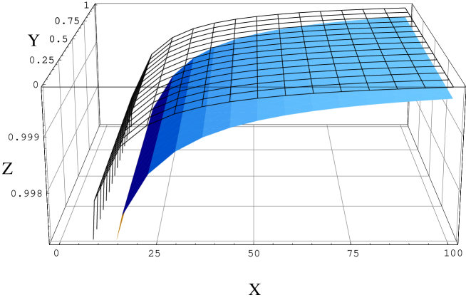
FIG. 1.: ${\cal E}_{\rm ELLPW}$ and ${\cal E}_{\rm KM}$ on Z-axis are plotted against ${\cal R}$ on X-axis and ${\cal S}$ on Y-axis for ${\cal Q}=0.2$. The upper (grid like) and lower surfaces are for ${\cal E}_{\rm ELLPW}$ and ${\cal E}_{\rm KM}$ respectively.

Now defining

$${\cal E}_{\rm ELLPW}:=\frac{E_{\rm ELLPW}}{M},\quad E_{\rm KM}:=E_{\rm K}=E_{\rm M\o l},\quad{\cal E}_{\rm KM}:=\frac{E_{\rm KM}}{M},$$ (22)

$${\cal S}:=\frac{a}{M},\quad{\cal Q}:=\frac{e}{M},\quad{\cal R}:=\frac{\rho}{M}$$ (23)

the equations $(\ref{EKomar})$, $(\ref{EELLPW})$ and $(\ref{EMol})$ may be expressed as

$${\cal E}_{\rm ELLPW}=1-\frac{{\cal Q}^{2}}{4{\cal R}}\left[1+\left(\frac{{\cal S}}{{\cal R}}+\frac{{\cal R}}{{\cal S}}\right)\arctan\left(\frac{{\cal S}}{{\cal R}}\right)\right]$$ (24)

and

$${\cal E}_{\rm KM}=1-\frac{{\cal Q}^{2}}{2{\cal R}}\left[1+\left(\frac{{\cal S}}{{\cal R}}+\frac{{\cal R}}{{\cal S}}\right)\arctan\left(\frac{{\cal S}}{{\cal R}}\right)\right]\text{\ .}$$ (25)

The ring curvature singularity in the KN metric is covered by the event horizon for $\left({\cal Q}^{2}+{\cal S}^{2}\right)\leq 1$ and is naked for $\left({\cal Q}^{2}+{\cal S}^{2}\right)>1$. In Fig. 1 we plot ${\cal E}_{\rm ELLPW}$ and ${\cal E}_{\rm KM}$ against ${\cal R}$ and ${\cal S}$ for ${\cal Q}=0.2$. As the value of ${\cal R}$ increases the two surfaces shown in the figure come closer.

IV Conclusions

The use of the Komar definition is not restricted to “Cartesian coordinates” (like one has for the ELLPW complexes); however, it is applicable only to the stationary space-times. The Møller energy-momentum complex is neither restricted to the use of particular coordinates nor to the stationary space-times. Lessner[18] pointed out that the Møller defintion is a powerful representation of energy and momentum in general relativity. However, one finds that for the Reissner-Nordström metric $E_{\rm ELLPW}=M-e^{2}/(2\rho)$ (the Penrose definition also gives the same result which agrees with linear theory[20] whereas $E_{\rm KM}=M-e^{2}/\rho$. Therefore, one prefers the results obtained by using the definitions of ETLLPW. It is worth investigating the Cooperstock hypothesis for non-static space-times with Møller’s energy-momentum complex.

- [1] C. W. Misner, K. S. Thorne and J. A. Wheeler, Gravitation (W. H. Freeman and Co., NY, 1973) p.603; F. I. Cooperstock and R. S. Sarracino, J. Phys. A11, 877 (1978); S. Chandrasekhar and V. Ferrari, Proceedings of Royal Society of London A435, 645 (1991).
- [2] H. Bondi, Proc. Roy. Soc. London A427, 249 (1990).
- [3] J. M. Aguirregabiria, A. Chamorro, and K. S. Virbhadra, Gen. Relativ. Gravit.. 28, 1393 (1996).
- [4] K. S. Virbhadra, Phys. Rev. D60, 104041 (1999).
- [5] C. Møller, Annals of Physics (NY) 4, 347 (1958).
- [6] C. Møller, Annals of Physics (NY) 12, 118 (1961); D. Kovacs, Gen. Relativ. Gravit. 17, 927 (1985); J. Novotny, Gen. Relativ. Gravit. 19, 1043 (1987).
- [7] A. Komar, Phy. Rev. 113, 934 (1959).
- [8] R. Penrose, Proc. Roy. Soc. London A381, 53 (1982).
- [9] J. D. Brown and J. W. York, Jr., Phys. Rev. D47, 1407 (1993).
- [10] S. A. Hayward, Phys. Rev. D49, 831 (1994).
- [11] G. Bergqvist, Class. Quantum Gravit. 9, 1753 (1992); D. H. Bernstein and K. P. Tod, Phys. Rev. D 49, 2808 (1994).
- [12] K. S. Virbhadra, Phys. Rev. D42, 1066 (1990); Phys. Rev. D42, 2919 (1990).
- [13] F. I. Cooperstock and S. A. Richardson, in Proc. 4th Canadian Conf. on General Relativity and Relativistic Astrophysics (World Scientific, Singapore, 1991).
- [14] K. S. Virbhadra, Phys. Lett. A157, 195 (1991); K. S. Virbhadra, Mathematics Today 9, 39 (1991); K. S. Virbhadra, Pramana - J. Phys. 38, 31 (1992); K. S. Virbhadra and J. C. Parikh, Phys. Lett. B317, 312 (1993); Phys. Lett. B331, 302 (1994); K. S. Virbhadra, Pramana - J. Phys. 44, 317 (1995); A. Chamorro and K. S. Virbhadra, Pramana - J. Phys. 45, 181 (1995); A. Chamorro and K. S. Virbhadra, Int. J. Mod. Phys. D5, 251 (1996); K. S. Virbhadra, Int. J. Mod. Phys. A12, 4831 (1997); S. S. Xulu, Int. J. Theor. Phys. 37, 1773 (1998); S. S. Xulu, Int. J. Mod. Phys. D7, 773 (1998).
- [15] N. Rosen and K. S. Virbhadra, Gen. Relativ. Gravit., 25, 429 (1993); K. S. Virbhadra, Pramana - J. Phys. 45, 215 (1995); N. Rosen, Gen. Relativ. Gravit., 26, 319 (1994); F. I. Cooperstock, Gen. Relativ. Gravit., 26, 323 (1994); F. I. Cooperstock and M. Israelit, Found. of Phys. 25, 631 (1995); N. Banerjee and S. Sen, Pramana-J. Physics, 49, 609 (1997); S. S. Xulu, Int. J. Theor. Phys (in press) gr-qc/9910015; S. S. Xulu, Int. J. Mod. Phys. A (in press), gr-qc/9902022.
- [16] C. C. Chang, J. M. Nester and C. Chen, Phys. Rev. Lett. 83, 1897 (1999).
- [17] J. M. Cohen, F. de Felice, J. Math. Phys.,25, 992 (1984).
- [18] G. Lessner, Gen. Relativ. Gravit. 28, 527 (1996).
- [19] F. I. Cooperstock, Mod. Phys. Lett. A14 1531 (1999).
- [20] K. P. Tod, Proc. Roy. Soc. London A388, 467 (1983).