To appear in Phys. Rev. D, July 15 (2001)
Complete null data for a black hole collision

Abstract

We present an algorithm for calculating the complete data on an event horizon which constitute the necessary input for characteristic evolution of the exterior spacetime. We apply this algorithm to study the intrinsic and extrinsic geometry of a binary black hole event horizon, constructing a sequence of binary black hole event horizons which approaches a single Schwarzschild black hole horizon as a limiting case. The linear perturbation of the Schwarzschild horizon provides global insight into the close limit for binary black holes, in which the individual holes have joined in the infinite past. In general there is a division of the horizon into interior and exterior regions, analogous to the division of the Schwarzschild horizon by the $r=2M$ bifurcation sphere. In passing from the perturbative to the strongly nonlinear regime there is a transition in which the individual black holes persist in the exterior portion of the horizon. The algorithm is intended to provide the data sets for production of a catalog of nonlinear post-merger wave forms using the PITT null code.

I Introduction

In previous work, we developed a model which generates the intrinsic null geometry of an event horizon with the “pair-of-pants” structure characteristic of a binary black hole merger [1, 2]. In this paper, we extend this approach to determine all extrinsic curvature properties of such horizons, thus providing a complete stand-alone description of the event horizon of binary black holes. We apply this work to study the event horizon of a head-on collision of black holes using a sequence of models which embraces not only the perturbative regime of the close approximation [3], where the merger takes place in the distant past, but also includes the highly nonlinear regime. In the perturbative regime the individual black holes merge in an interior region of the horizon, corresponding to the region of the Schwarzschild event horizon lying inside the $r=2M$ bifurcation sphere. But we show how dramatically nonlinear effects can push the merger into the exterior portion of the horizon.

Beyond the investigation of the horizon geometry of a black hole collision, the major motivation for this work is to provide the null data necessary to compute the emitted gravitational wave by means of a characteristic evolution of the exterior spacetime. In the Cauchy problem, the necessary data on a spacelike hypersurface are the intrinsic metric and extrinsic curvature, subject to constraints. On a null hypersurface, such as an event horizon, the situation is quite different. The necessary null data consist of the conformal part of the intrinsic (degenerate) metric, which can be given freely as a function of the affine parameter. Then the surface area of the horizon is determined, via an ordinary differential equation along the null rays (the Raychaudhuri equation), in terms of an integration constant supplied by the mass of the final black hole. Similarly, all extrinsic curvature components of the horizon are determined by ordinary differential equations in terms of integration constants supplied by the final black hole. Whereas in principle the intrinsic conformal geometry is the only data on the horizon necessary for the characteristic initial value problem, in practice the surface area and extrinsic curvature are essential to supply the start-up data for the implementation of a characteristic evolution code, such as the PITT null code [4, 5]. The main results of this paper concern the understanding of the nonlinear nature of the underlying ordinary differential equations from geometrical, physical and numerical points of view.

Given the intrinsic geometry and extrinsic curvature of the horizon, the strategy behind the characteristic approach to the computation of the emitted wave has been outlined elsewhere [6]. It consists of two evolution stages based upon the double null initial value problem. Referring to Fig. 1, the necessity of two stages results from the disconnected nature of the two null hypersurfaces on which boundary conditions must be satisfied: (i) the event horizon ${\cal H}^{+}$, where binary black hole data is prescribed, and (ii) past null infinity ${\cal I}^{-}$, where ingoing radiation must be absent, at least in the late stage to the future of the hypersurface $\Gamma$ which is decoupled from the formation of the individual black holes. Rather than directly attempting to solve this mixed version of a characteristic initial value problem, the stage I evolution is based upon two intersecting null hypersurfaces consisting of the event horizon, where binary black hole data is prescribed, and an ingoing null hypersurface ${\cal J}^{+}$ approximating future null infinity ${\cal I}^{+}$, where data corresponding to no outgoing radiation is prescribed. The characteristic evolution then proceeds backward in time along ingoing null hypersurfaces extending to ${\cal I}^{-}$ to determine the spacetime exterior to an ingoing null hypersurface $\Gamma$. As indicated in the figure, the evolution terminates at $\Gamma$ because the horizon splits into two individual black holes. This stage I solution is the advanced solution to the problem in the sense that radiation from ${\cal I}^{-}$ is absorbed by the black holes but no outgoing wave is radiated to ${\cal I}^{+}$. Stage II provides the retarded solution, where outgoing but no ingoing radiation is present outside $\Gamma$, by running forward in time a double null evolution based upon the intersecting null hypersurfaces $\Gamma$, where the stage I data is prescribed, and an outgoing null hypersurface ${\cal J}^{-}$ approximating ${\cal I}^{-}$, where data corresponding to no ingoing radiation is prescribed to the future of $\Gamma$. The stage II evolution produces the retarded solution for the spacetime outside the world tube $\Gamma$. The approach is a nonlinear version of the standard method of determining the retarded solution $\Phi_{RET}$ of the linear wave equation $\Box\Phi=S$, with source $S$, by first finding the advanced solution $\Phi_{ADV}$ and then superimposing the source-free solution $\Phi_{RET}-\Phi_{ADV}$. In the nonlinear case, where standard Green function techniques cannot be used to define retarded and advanced solutions, they can be defined by requiring the absence of radiation at ${\cal I}^{+}$ (retarded) or ${\cal I}^{-}$ (advanced). In the present case, the data on the world tube $\Gamma$ represents the interior source which has led to the formation of the individual black holes. (In a normal physical context, the source consists of two stars undergoing gravitational collapse but in a purely vacuum scenario imploding gravitational waves can play the role of the matter.) The justification of this two stage approach is that it reduces to the standard linear method in the close approximation where the geometry can be regarded as a perturbation of a Schwarzschild background. A purely perturbative characteristic treatment of the close approximation using the characteristic approach has been carried out in a separate study and the advanced solution has been successfully computed [7].

We intend to carry out the “backward in time” evolution using the PITT null code [4, 5], which is based upon the Bondi-Sachs version of the characteristic initial value problem [8, 9]. The present code is designed to evolve forward in time along a foliation of spacetime by outgoing null hypersurfaces. In this paper, in order to apply it to the backward in time evolution of a black hole horizon, we describe the merger of two black holes in the time reversed scenario of a white hole horizon, in which the black hole merger is now represented by the fission of a white hole. The post-merger era of the black hole horizon then corresponds to the pre-fission era of the white hole; and the proposed backward in time evolution of the black hole horizon to determine the exterior spacetime corresponds to a forward in time evolution of the white hole horizon. Our algorithm provides the complete white hole data necessary to carry out this evolution.

The specific application in this paper is to the axisymmetric head-on collision of two equal mass black holes. However, the algorithm is capable of generating intrinsic geometry and extrinsic curvature of an arbitrary event horizon, including the case of inspiraling binary black holes of non-equal mass. In previous studies of the intrinsic geometry of non-axisymmetric horizons, the approach has revealed new features of the generic collision of two black holes, such as an intermediate toroidal phase which precedes the merger [2]. Here we apply the algorithm to gain new insight into the global behavior of the extrinsic curvature properties of the head-on collision.

The material in the paper divides into two types: (i) general features of a binary horizon and (ii) the calculation of the null data on the horizon necessary to initiate the PITT code. Material of the first type, which describes how a binary horizon deviates from the close approximation in the nonlinear regime, appears in Secs. II A and III - VI and can be read independently. This material is described most conveniently in terms of Sachs coordinates, introduced in Sec. II A. Material of the second type involves the transformation from Sachs to Bondi-Sachs coordinates, introduced in Sec. II B. This material supplies all data necessary to compute, using the PITT code, the fully nonlinear merger to ringdown wave form, which will be the subject of future work. The details of implementing the horizon data algorithm as a finite difference code are given in the Appendixes. An independent code designed for an axisymmetric horizon is also described and has been used as an independent test of the full code.

We retain the conventions of our previous papers [1, 2, 4, 5], with only minor changes in notation where noted in the text. For brevity, we frequently use the notation $f_{,x}=\partial_{x}f$ to denote partial derivatives and $\dot{f}=\partial_{u}f$ to denote retarded time derivatives.

II Characteristic data on a horizon

A Horizon structure

The evolution of the exterior spacetime by the PITT code proceeds along a family of outgoing null hypersurfaces. The characteristic initial value problem for the evolution requires an inner boundary condition which can be set either on a timelike world tube or, as a limiting case, on a null world tube. Here we choose the inner boundary to be the null world tube representing a white hole horizon ${\cal H}$. The white hole horizon pinches off in the future where its generators either caustic or cross each other (such as at the vertex of a null cone). As illustrated in Fig. 2, we introduce (i) an affine null coordinate $u$ along the generators of ${\cal H}$, which foliates ${\cal H}$ into cross sections ${\cal S}_{u}$ and labels the corresponding outgoing null hypersurfaces ${\cal J}_{u}$ emanating from the foliation; (ii) angular coordinates $x^{A}$ which are constant both along the generators of ${\cal H}$ and along the outgoing rays and (iii) an affine parameter $\lambda$ along the outgoing rays normalized by $\nabla^{\alpha}u\nabla_{\alpha}\lambda=-1$, with $\lambda=0$ on ${\cal H}$. In the resulting $x^{\alpha}=(u,\lambda,x^{A})$ coordinates, the metric takes the form

$$ds^{2}=-(W-g_{AB}W^{A}W^{B})du^{2}-2dud\lambda-2g_{AB}W^{B}dudx^{A}+g_{AB}dx^{A}dx^{B}.$$ (1)

The contravariant components are given by $g^{\lambda u}=-1$, $g^{\lambda A}=-W^{A}$, $g^{\lambda\lambda}=W$ and $g^{AB}g_{BC}=\delta^{A}_{C}$. In addition, we set $g_{AB}=r^{2}h_{AB}$, where $\det(h_{AB})=\det(q_{AB})=q(x^{A})$, where $q_{AB}$ is some standard choice of unit sphere metric.

These coordinates were first introduced by Sachs to formulate the double-null characteristic initial value problem [10]. The Bondi-Sachs coordinate system  [8, 9] used in the PITT code differs by the use of a surface area coordinate $r$ along the outgoing cones rather than the affine parameter $\lambda$. However, because the horizon is not a surface of constant $r$, except in the special case of an “isolated horizon” [11], it is advantageous to first determine the necessary data in terms of an affine parameter and later transform to the $r$-coordinate.

The requirement that ${\cal H}$ be null implies that $W=0$ on ${\cal H}$. There is gauge freedom on ${\cal H}$ that we fix by choosing the shift so that $\partial_{u}$ is tangent to the generators, implying that $W^{A}=0$ on ${\cal H}$; and by choosing the lapse so that $u$ is an affine parameter, implying that $\partial_{\lambda}W=0$ on ${\cal H}$. We adopt these choices throughout the paper, and our results generally hold only on $\cal H$ ($\lambda=0$) and when these conditions are satisfied. Later, in Sec. IV, we also fix the affine freedom in $u$ by specifying it on an initial slice ${\cal S}^{-}$ of ${\cal H}$, which is located at an early time approximating the asymptotic equilibrium of the white hole at past time infinity $I^{-}$. The outgoing null hypersurface ${\cal J}^{-}$ emanating from ${\cal S}^{-}$ approximates past null infinity ${\cal I}^{-}$. In Sec.  IV B, we discuss the nature of that approximation.

On ${\cal H}$, the affine tangent to the generators $n^{a}\partial_{a}=\partial_{u}$ (see Fig. 2) satisfies the geodesic equation $n^{b}\nabla_{b}n^{a}=0$ and the hypersurface orthogonality condition $n^{[a}\nabla^{b}n^{c]}=0$. Following the approach of Refs. [1, 2], we project 4-dimensional tensor fields into ${\cal H}$ using the operator

$$P_{a}^{b}=\delta_{a}^{b}+n_{a}l^{b},$$ (2)

where $l_{a}=-\nabla_{a}u$, and we use the shorthand notation $\perp T_{a}^{b}$ for the projection (to the tangent space of ${\cal H}$) of the tensor field $T_{a}^{b}$. The projection $\perp$ has gauge freedom corresponding to the choice of affine parameter $u$. However, the action of $\perp$ on covariant indices is independent of this freedom and equals the action of the pullback operator to ${\cal H}$.

In addition to the intrinsic geometry of ${\cal H}$, the necessary characteristic data consist of the extrinsic curvature quantities given by $\perp\nabla_{a}l_{b}$ (with gauge freedom corresponding to the affine choice of $u$). Since $\nabla_{a}l_{b}-\nabla_{b}l_{a}=0$, the independent components are determined by $\perp\nabla_{(a}l_{b)}$, which has the decomposition

$$\perp\nabla_{(a}l_{b)}=-l_{a}\omega_{b}-\omega_{a}l_{b}+\tau_{ab}.$$ (3)

Here $\tau_{ab}$ describes the shear and expansion of the outgoing rays and satisfies $n^{a}\tau_{ab}=0$ on ${\cal H}$. Following Hayward [12], we call $\omega_{a}=\perp n^{b}\nabla_{b}l_{a}$ the twist of the affine foliation of ${\cal H}$. The twist also satisfies $n^{a}\omega_{a}=0$. Unlike $\tau_{ab}$, the twist is an invariantly defined extrinsic curvature property of the $u=const$ cross sections of ${\cal H}$, independent of the boost freedom in the extensions of $n_{a}$ and $l_{a}$ subject to the normalization $n^{a}l_{a}=-1$.

Note that it is natural geometrically to associate extrinsic curvature properties of ${\cal H}$ with $(\perp\nabla_{a})n^{b}$, in analogy with the Weingarten map for a non-degenerate hypersurface [11]. The normalization $n^{a}l_{a}=-1$ then leads, via Eq. (3), to

$$l_{b}(\perp\nabla_{a})n^{b}=-\omega_{a}.$$ (4)

Thus the twist describes an extrinsic curvature property associated with $n^{a}$ as well as $l_{a}$. The other components of $(\perp\nabla_{a})n^{b}$ are determined by the shear and expansion of ${\cal H}$ (which vanish in the special case of an isolated horizon).

We consider the double null initial value problem based upon data on the horizon ${\cal H}$ and the outgoing null hypersurface ${\cal J}^{-}$ emanating from ${\cal S}^{-}$, with the evolution proceeding along the outgoing null hypersurfaces ${\cal J}_{u}$ emanating from the $u=const$ foliation ${\cal S}_{u}$. In this problem, the complete (and unconstrained) characteristic data on ${\cal H}$ are its affine parametrization $u$ and the conformal part $h_{AB}$ of its degenerate intrinsic metric. Similarly, the characteristic data on ${\cal J}^{-}$ are its affine parametrization $\lambda$ and its intrinsic conformal metric $h_{AB}$. The remaining data consist of the intrinsic metric and extrinsic curvature of ${\cal S}^{-}$ (subject to consistency with the characteristic data) [10, 13]. In Sachs coordinates, this data on ${\cal S}^{-}$ consists of $r$, $\dot{r}$, $\omega_{a}$ and $r_{,\lambda}$ (which determines the expansion of the outgoing null rays) on ${\cal S}^{-}$. That completes the data necessary to evolve the exterior spacetime. In carrying out such an evolution computationally, the first step is to propagate the data given on ${\cal S}^{-}$ along the generators of ${\cal H}$ so that it can be supplied as boundary data to the exterior evolution code. This first step is accomplished by means of certain components of Einstein’s equations.

Einstein’s equation decompose into (i) hypersurface equations intrinsic to the null hypersurfaces ${\cal J}_{u}$, which determine auxiliary metric quantities in terms of the conformal metric $h_{AB}$; (ii) evolution equations determining the rate of change $\partial_{u}h_{AB}$ of the conformal metric of ${\cal J}_{u}$; and (iii) propagation equations which are constraints that need only be satisfied on ${\cal H}$. One of the propagation equations is the ingoing Raychaudhuri equation $R_{uu}=0$ which determines the surface area variable $r$ along the generators of ${\cal H}$ in terms of initial conditions on ${\cal S}^{-}$ according to

$$\ddot{r}=\frac{r}{8}\dot{h}^{AB}\dot{h}_{AB}.$$ (5)

The value of $\dot{r}$ on ${\cal S}^{-}$ measures the convergence of its ingoing null rays and Eq. (5) implies $\ddot{r}\leq 0$. The remaining propagation equations $R_{Au}=0$ propagate the twist $\omega_{a}$ along the generators of ${\cal H}$. Our coordinate conditions imply that $\omega_{u}=\omega_{\lambda}=0$ and

$$\omega_{A}=-\frac{1}{2}\partial_{\lambda}(g_{AB}W^{B}).$$ (6)

The non-vanishing components propagate according to

$$(r^{2}\omega_{A})\dot{}=r^{2}D_{A}(\frac{\dot{r}}{r})-\frac{1}{2}h^{BC}D_{B}(r^{2}\dot{h}_{AC}),$$ (7)

where $D_{A}$ is the covariant derivative associated with $h_{AB}$. Here $h^{AB}h_{BC}=\delta^{A}_{C}$ and $h^{AB}\dot{h}_{AB}=0$. Having determined $r$, this equation can easily be integrated to determine $\omega_{A}$ on ${\cal H}$ in terms of initial conditions on ${\cal S}^{-}$. Once the propagation equations are solved on ${\cal H}$ to determine $r$ and $\omega_{a}$, the Bianchi identities ensure that they will be satisfied in the exterior spacetime as a result of the ${\cal J}_{u}$ hypersurface equations and the evolution equations.

The propagation of $\tau_{ab}$ (the outward shear expansion and shear) along ${\cal H}$ requires the $R_{AB}=0$ components of Einstein equations, given by

$$R_{AB} = h_{AB}\bigg{(}\frac{{\cal R}}{2}-D^{A}D_{A}\,\log r\bigg{)}-D_{A}\omega_{B}-D_{B}\omega_{A}-2\omega_{A}\omega_{B}$$ (8)

$$+ \frac{2}{r}(\omega_{A}\partial_{B}r+\omega_{B}\partial_{A}r-h_{AB}h^{CD}\omega_{C}\partial_{D}r)$$ (9)

$$+ r^{2}\partial_{\lambda}\dot{h}_{AB}-\frac{r^{2}}{2}h^{CD}(\dot{h}_{AC}\partial_{\lambda}h_{BD}+\dot{h}_{BD}\partial_{\lambda}h_{AC})$$ (10)

$$+ 2(\dot{r}\partial_{\lambda}r+r\partial_{\lambda}\dot{r})h_{AB}+r(\partial_{\lambda}r)\dot{h}_{AB}+r\dot{r}\partial_{\lambda}h_{AB}.$$ (11)

where ${\cal R}$ represents the curvature scalar of the metric $h_{AB}$. On ${\cal H}$, the equation $R_{AB}=0$ decomposes into the trace

$$\partial_{u}\partial_{\lambda}(r^{2})=+D^{A}D_{A}\,\log r-\frac{1}{2}{\cal R}+D^{A}\omega_{A}+h^{AB}\omega_{A}\omega_{B}$$ (12)

and, by introducing the dyad decomposition $h_{AB}=m_{(A}\bar{m}_{B)}$, the trace-free part

$$m^{A}m^{B}\bigg{(}r\partial_{\lambda}\partial_{u}(rh_{AB})-2D_{A}\omega_{B}-2\omega_{A}\omega_{B}+\frac{4}{r}\omega_{A}D_{B}r\bigg{)}=0.$$ (13)

The trace equation propagates the outgoing expansion of the foliation ${\cal S}_{u}$, as determined by $r_{,\lambda}$. The trace-free part is the evolution equation for the data $h_{AB}$ on the foliation ${\cal J}_{u}$, applied at ${\cal H}$ to evolve $h_{AB,\lambda}$, which describes the shear of the outgoing rays. The outward shear constitutes part of the extrinsic curvature of ${\cal S}^{-}$. Although its value is implicitly determined by the null data $h_{AB}$ on ${\cal J}^{-}$, we view it as part of the initial data that must be specified on ${\cal S}^{-}$.

In summary, the data for the double null problem includes the conformal metric on ${\cal H}$ and the quantities $r$, $\dot{r}$, $\omega_{a}$, $r_{,\lambda}$ and $h_{AB,\lambda}$ on ${\cal S}^{-}$. Equations (5), (7), (12) and (13) are then used to propagate the data on ${\cal S}^{-}$ to all of ${\cal H}$. The choice of foliation of the horizon is an important but complicated aspect of this problem. As in the case of Cauchy evolution, gauge freedom in the foliation introduces arbitrariness into the dynamical description of any black hole process and, in particular, the pair-of-pants structure underlying a black hole merger. In the case of the horizon, the natural choice of an affine foliation $u$ removes any time dependence from this gauge freedom but there remains the affine freedom $u\rightarrow Au+B$, where $A$ and $B$ are ray dependent. In Sec. IV, we use the asymptotic equilibrium of the white hole as $u\rightarrow-\infty$ to fix this freedom. We review in Sec. III how the data $h_{AB}$ and $r$ on ${\cal H}$ describing a white hole fission (binary black hole merger) are provided by a conformal horizon model[1, 2]. The additional data required on ${\cal S}^{-}$ can be inferred from the asymptotic properties of the white hole equilibrium at $I^{-}$, as discussed in Sec. IV. The evolution of the exterior spacetime by the PITT code requires a transformation of the data on ${\cal H}$ to a Bondi-Sachs coordinate system, as described next in Secs. II B - II D.

B Bondi-Sachs coordinates

The transformation to the Bondi-Sachs coordinates $x^{\alpha}=(u,r,x^{A})$ used in the PITT code consists in substituting the surface area coordinate $r$ for the affine parameter $\lambda$. Since the horizon ${\cal H}$ does not in general have constant $r$ it does not lie precisely on radial grid points. Consequently, the assignment of horizon boundary values must be done on the grid points nearest to the boundary. Thus an accurate prescription of boundary conditions in the $r$-grid requires a Taylor expansion of the horizon data.

In Bondi-Sachs variables, the resulting metric takes the form

$$ds^{2}=-\left(e^{2\beta}{V\over r}-r^{2}h_{AB}U^{A}U^{B}\right)du^{2}-2e^{2\beta}dudr-2r^{2}h_{AB}U^{B}dudx^{A}+r^{2}h_{AB}dx^{A}dx^{B}.$$ (14)

In relating this to the Sachs metric Eq. (1), it is simplest to consider the contravariant form in which only the $g^{r\alpha}$ components differ. In terms of the corresponding metric variables,

$$g^{rr} =e^{-2\beta}\frac{V}{r} =(r_{,\lambda})^{2}W-2\,r_{,\lambda}r_{,A}W^{A}-2\,r_{,\lambda}r_{,u}+\frac{r_{,A}r_{,B}}{r^{2}}h^{AB}$$ (15)

$$g^{rA} =-e^{-2\beta}U^{A} =-r_{,\lambda}W^{A}+\frac{r_{,B}}{r^{2}}h^{AB}$$ (16)

$$g^{ru} =-e^{-2\beta} =-r_{,\lambda}.$$ (17)

Restricted to ${\cal H}$, our choice of lapse and shift imply

$$\beta = -\frac{1}{2}\ln{r_{,\lambda}}$$ (18)

$$U^{A} = -\frac{e^{2\beta}}{r^{2}}r_{,B}h^{AB}$$ (19)

$$V = -2\,rr_{,u}+\frac{e^{2\beta}}{r}r_{,A}r_{,B}h^{AB}.$$ (20)

The structure of the ${\cal J}_{u}$-hypersurface equations and the evolution equations [14, 15] reveals the horizon boundary data necessary for characteristic evolution. The hypersurface equations are

$$\beta_{,r} = \frac{1}{16}rh^{AC}h^{BD}h_{AB,r}h_{CD,r},$$ (21)

$$(r^{4}e^{-2\beta}h_{AB}U^{B}_{,r})_{,r} = 2r^{4}\left(r^{-2}\beta_{,A}\right)_{,r}-r^{2}h^{BC}D_{C}h_{AB,r}$$ (22)

$$2e^{-2\beta}V_{,r} = {\cal R}-2D^{A}D_{A}\beta-2D^{A}\beta D_{A}\beta+r^{-2}e^{-2\beta}D_{A}(r^{4}U^{A})_{,r}$$ (23)

$$- \frac{1}{2}r^{4}e^{-4\beta}h_{AB}U^{A}_{,r}U^{B}_{,r}\,,$$ (24)

where here $D_{A}$ is the covariant derivative and ${\cal R}$ the curvature scalar of the 2-metric $h_{AB}$ of the $r=const$ surfaces (which differ from the corresponding quantities on the $\lambda=const$ surfaces). These equations form a hierarchy which can be integrated radially in order to determine $\beta$, $U^{A}$ and $V$ on a hypersurface ${\cal J}_{u}$ in terms of integration constants on ${\cal S}_{u}$, once the null data $h_{AB}$ has been evolved to ${\cal J}_{u}$.

The evolution variable $h_{AB}$ can be recast as a single complex function, since $\det(h_{AB})=\det(q_{AB})=q(x^{A})$ is independent of $u$ and $r$. The code treats such functions on the sphere in terms of stereographic angular coordinates based upon the auxiliary unit sphere metric $q_{AB}$. Tensor fields are represented by spin-weighted functions using a computational version of the $\eth$-formalism [16] based upon a complex dyad $q_{A}$, satisfying $q_{AB}=q_{(A}\bar{q}_{B)}$. (Note that this departs from other conventions [17] in order to avoid unnecessary factors of $\sqrt{2}$ which would be awkward in numerical work.) For example, the vector field $v_{A}$ is represented by the spin-weight 1 function $v=q^{A}v_{A}$. Derivatives of tensor fields are represented by $\eth$ operators on spin-weighted functions by taking dyad components of covariant derivatives with respect to the unit sphere metric. Our conventions are fixed in the case of a scalar field $\Psi$ by $\eth\Psi=q^{A}\nabla_{A}\Psi$. In these conventions,

$$(\bar{\eth}\eth-\eth\bar{\eth})\eta=2s\eta$$ (25)

for a spin-weight $s$ field $\eta$.

The conformal metric $h_{AB}$ is represented by the dyad components $J=h_{AB}q^{A}q^{B}/2$ and $K=h_{AB}q^{A}\bar{q}^{B}/2$, with the determinant condition implying $K^{2}=1+J\bar{J}$. As discussed in [16], the curvature scalar corresponding to $h_{AB}$ is

$${\cal R}=2K-\eth\bar{\eth}K+{1\over 2}[\bar{\eth}^{2}J+\eth^{2}\bar{J}]+{1\over 4K}[\bar{\eth}\bar{J}\eth J-\bar{\eth}J\eth\bar{J}].$$ (26)

In terms of $J$, the evolution equation takes the form

$$2\left(rJ\right)_{,ur}-\left(r^{-1}V\left(rJ\right)_{,r}\right)_{,r}=S_{J}$$ (27)

where $S_{J}$ is explicitly given in term of spin-weighted fields in Ref. [4]. $S_{J}$ contains only first derivatives of $J$ and predetermined hypersurface quantities so that it does not play a major role in the integration of Eq. (27) on a given null hypersurface ${\cal J}_{u}$.

Similarly, in integrating Eq. (22) for $U^{A}$, the code uses the spin-weight 1 fields $U=q_{A}U^{A}$ and $Q=q^{A}Q_{A}$, where

$$Q_{A}=r^{2}e^{-2\,\beta}h_{AB}U^{B}_{,r},$$ (28)

so that Eq. (22) reduces to the first order radial equations

$$\left(r^{2}Q\right)_{,r} = q^{A}[2r^{4}\left(r^{-2}\beta_{,A}\right)_{,r}-r^{2}h^{BC}D_{C}h_{AB,r}],$$ (29)

$$U_{,r} = r^{-2}e^{2\beta}q_{A}h^{AB}Q_{B},$$ (30)

with the right-hand sides then rewritten in the $\eth$-formalism in terms of spin-weighted fields.

The integration constants necessary to evolve Eqs. (21) - (27) are the boundary values of $r$, $J$, $\beta$, $Q$, $U$ and $V$ on ${\cal H}$. Part of these boundary conditions are determined by the characteristic data on ${\cal H}$ and the remainder are determined by gauge conditions and the solution of the propagation equations. When the horizon ${\cal H}$ has constant $r$ (as in the Schwarzschild case), this is precisely the data necessary to initiate the radial integrations in the PITT code. In the generic case, ${\cal H}$ does not lie on grid points and the initialization of the $r$-grid boundary also requires $\partial_{r}J$, $\partial_{r}\beta$ and $\partial_{r}V$ on ${\cal H}$ to provide a Taylor expansion consistent with a second order accurate code..

C From horizon variables to Bondi metric functions

We now describe the calculation of the Bondi-Sachs metric variables in a neighborhood of the horizon as necessary for a characteristic evolution of the exterior space-time. The essential piece of free horizon data is the conformal metric $h_{AB}$ or equivalently the metric function $J$. In Sec. III, this data is supplied for the case of a binary horizon by the conformal model, in which case the value of $r$ on the horizon is also supplied. In a more general situation, where only $J$ is prescribed, $r$ can be determined from its value and time derivative $\dot{r}$ on $S^{-}$ using the ingoing Raychaudhuri equation (5), which in spin-weighted form is

$$\ddot{r}=-\frac{r}{4}(\dot{J}\dot{\bar{J}}-\dot{K}^{2}).$$ (31)

Here, we have used the dyad expansion of the conformal metric $h^{AB}$ which can be written in terms of $J$ and $K$ as

$$2\,h^{AB}=-\bar{J}q^{A}q^{B}-J\bar{q}^{A}\bar{q}^{B}+K\left(q^{A}\bar{q}^{B}+\bar{q}^{A}q^{B}\right).$$ (32)

Once both the intrinsic geometry $J$ and the radial coordinate $r$ are known, the metric functions $\beta$, $U$ and $W$ (as well as their radial derivatives) can be calculated using a hierarchy of horizon propagation equations [similar to the hierarchy of hypersurface and evolution equations (18)-(27) used to propagate fields along a ${\cal J}_{u}$ null hypersurface].

Next in this hierarchy is the propagation Eq. (7) for the twist $\omega=q^{A}\omega_{A}$ , which has spin-weighted form

$$(r^{2}\omega)\dot{} = r^{2}\eth(\frac{\dot{r}}{r})+\frac{1}{2}[J\bar{\eth}(r^{2}\dot{K})+\bar{J}\eth(r^{2}\dot{J})-K\bar{\eth}(r^{2}\dot{J})-K\eth(r^{2}\dot{K})]$$ (33)

$$+ \frac{r^{2}}{4}(\dot{\bar{J}}\eth J-4\dot{K}\eth K+2\dot{K}\bar{\eth}J+3\dot{J}\eth\bar{J}-2\dot{J}\bar{\eth}K)$$ (34)

and determines $\omega$ given its initial value on the slice $S^{-}$ and the conformal horizon geometry encoded in $J$.

Next, the value of $\beta$ follows from Eq. (18) with $r_{,\lambda}$ determined from Eq. (12) in the spin-weighted form

$$\partial_{u}\partial_{\lambda}(r^{2}) = \frac{1}{2}\bar{\eth}[K(\eth\log r+\omega)]+\frac{1}{2}\eth[K(\bar{\eth}\log r+\bar{\omega})]-\frac{1}{2}\bar{\eth}[J(\bar{\eth}\log r+\bar{\omega})]-\frac{1}{2}\eth[\bar{J}(\eth\log r+\omega)]$$ (35)

$$- \frac{1}{2}{\cal R}-\frac{1}{2}J\bar{\omega}^{2}-\frac{1}{2}\bar{J}\omega^{2}+K\omega\bar{\omega},$$ (36)

where Eq. (26) supplies the spin-weighted form of the curvature scalar ${\cal R}$ of the metric $h_{AB}$. This determines $r_{,\lambda}$ on the entire horizon given its value on the initial slice $S^{-}$.

Next, the Bondi metric functions $U$ and $V$ are evaluated on the horizon using Eqs. (19) and (20) in the spin-weighted forms

$$U = \frac{e^{2\beta}}{r^{2}}\left(J\bar{\eth}r-K\eth r\right)$$ (37)

$$V = -2\,rr_{,u}+\frac{e^{2\beta}}{2r}\left(-\bar{J}\left(\eth r\right)^{2}-J\left(\bar{\eth}r\right)^{2}+2\,K\left(\eth r\right)\left(\bar{\eth}r\right)\right).$$ (38)

In summary, the Bondi metric functions $r$, $J$, $\beta$, $U$ and $V$ are determined by the hierarchy of Eqs. (31) and (34) - (38). When the value of $r$ is given, as in the conformal model, Eq. (31) is not needed.

D Extending the Bondi metric off the horizon

The evaluation of the Bondi metric functions on radial grid points in the neighborhood of the horizon requires the $r$-derivatives of $J$, $\beta$, $U$ and $V$. For this purpose we note that, on any given ray, the quantity $\partial_{r}F$ is known once both $\partial_{\lambda}F$ and $r_{,\lambda}$ are determined, e.g.

$$\partial_{r}J=\partial_{\lambda}J/r_{,\lambda}=e^{2\beta}\partial_{\lambda}J.$$ (39)

We assume below that $r_{,\lambda}$ has already been determined on the horizon by integrating Eq. (36).

We obtain $J_{,r}$ on the horizon (and hence $K_{,r}$) in terms of $\partial_{\lambda}J$, which is determined from its initial value on $S^{-}$ by integrating Eq. (13) in the spin-weighted form

$$0 = 2r^{2}\partial_{u}\partial_{\lambda}J+2r\dot{r}\partial_{\lambda}J+2r\dot{J}\partial_{\lambda}r-Jr^{2}(\dot{\bar{J}}\partial_{\lambda}J+\dot{J}\partial_{\lambda}\bar{J}-2\dot{K}\partial_{\lambda}K)$$ (40)

$$- (1+K^{2})(\eth\omega+\omega^{2}-2\omega\eth\log r)+\omega(J\bar{\eth}K-K\bar{\eth}J)+\bar{\omega}(K\eth J-J\eth K)$$ (41)

$$- J\bigg{(}J\bar{\eth}\bar{\omega}-K(\eth\bar{\omega}+\bar{\eth}\omega)+J\bar{\omega}^{2}-2K\omega\bar{\omega}+2K(\omega\bar{\eth}\log r+\bar{\omega}\eth\log r)-2J\bar{\omega}\bar{\eth}\log r\bigg{)}.$$ (42)

We calculate $\beta_{,r}$ from the Raychaudhuri equation for the outgoing null geodesics, $R_{\lambda\lambda}=0$, which in Sachs coordinates takes the form

$$r_{,\lambda\lambda}=-\frac{r}{8}h^{AC}h^{BD}h_{AB,\lambda}h_{CD,\lambda}\,,$$ (43)

with spin-weighted version

$$r_{,\lambda\lambda}=\frac{r}{4}\left(\left(K_{,\lambda}\right)^{2}-J_{,\lambda}\bar{J}_{,\lambda}\right),$$ (44)

which, together with Eq. (18), gives

$$\beta_{,r}=\frac{r}{8}(J_{,r}\bar{J}_{,r}-K_{,r}^{2}).$$ (45)

We obtain $U_{,r}$ (or $Q$) from the twist, which in Bondi coordinates takes the form

$$\omega_{A}=\partial_{A}\beta+\frac{1}{r}\partial_{A}r+\frac{1}{2}\partial_{r}(h_{AB})h^{BC}\partial_{C}r-\frac{r^{2}}{2}e^{-2\beta}h_{AB}\partial_{r}U^{B},$$ (46)

with spin-weighted version

$$\omega=\eth\beta+\frac{1}{r}\eth r+\frac{1}{2}(\partial_{r}J)(K\bar{\eth}r-\bar{J}\eth r)+\frac{1}{2}(\partial_{r}K)(K\eth r-J\bar{\eth}r)-\frac{Q}{2}.$$ (47)

This determines the boundary data for $Q$ in terms of quantities that are already known on the horizon. Given $Q$, the value of $\partial_{r}U$ follows from Eq. (30), which has spin-weighted form

$$U_{,r}=\frac{e^{2\beta}}{r^{2}}\left(KQ-J\bar{Q}\right).$$ (48)

Finally, we compute $\partial_{r}V$ by obtaining $V_{,\lambda}$ from the $\lambda$-derivative of Eq. (15),

$$\frac{e^{-2\beta}}{r}\left[V_{,\lambda}-V\left(2\,\beta_{,\lambda}+\frac{r_{,\lambda}}{r}\right)\right] = (r_{,\lambda})^{2}_{,\lambda}W+(r_{,\lambda})^{2}W_{,\lambda}-2\,\left(r_{,\lambda}r_{,A}\right)_{,\lambda}W^{A}-2\,r_{,\lambda}r_{,A}W^{A}_{,\lambda}$$ (49)

$$- 2\,r_{,\lambda\lambda}r_{,u}-2\,r_{,\lambda}r_{,\lambda u}+2\,\frac{r_{,\lambda A}r_{,B}}{r^{2}}h^{AB}-2\,\frac{r_{,\lambda}r_{,A}r_{,B}}{r^{3}}h^{AB}$$ (50)

$$+ \frac{r_{,A}r_{,B}}{r^{2}}h^{AB}_{,\lambda}.$$ (51)

The first three terms in the right-hand side vanish on ${\cal H}$ due to the gauge conditions. We express the others in spin-weighted form using Eq. (6) to obtain

$$-2\,r_{,A}W^{A}_{,\lambda}=\frac{2}{r^{2}}\left(-\bar{J}\omega\eth r-J\bar{\omega}\bar{\eth}r+K\left(\bar{\omega}\eth r+\omega\bar{\eth}r\right)\right)$$ (52)

and Eq. (32) to obtain

$$2\,r_{,\lambda A}r_{,B}h^{AB} = -\bar{J}(\eth r_{,\lambda})(\eth r)-J(\bar{\eth}r_{,\lambda})(\bar{\eth}r)+K\left((\eth r_{,\lambda})(\bar{\eth}r)+(\bar{\eth}r_{,\lambda})(\eth r)\right)$$ (53)

$$2\,r_{,A}r_{,B}h^{AB}_{,\lambda} = -\bar{J}_{,\lambda}(\eth r)^{2}-J_{,\lambda}(\bar{\eth}r)^{2}+2\,K_{,\lambda}(\eth r)(\bar{\eth}r).$$ (54)

Then Eq. (51) gives

$$V_{,\lambda} = V\left(2\,\beta_{,\lambda}+\frac{e^{-2\beta}}{r}\right)+4\,r\,r_{,u}\beta_{,\lambda}-2\,r\,r_{,\lambda u}+\frac{2}{r}\left(-\bar{J}\omega\eth r-J\bar{\omega}\bar{\eth}r+K\left(\bar{\omega}\eth r+\omega\bar{\eth}r\right)\right)$$ (55)

$$+ \frac{e^{2\beta}}{r}\left(-\bar{J}\left(\eth r_{,\lambda}\right)\left(\eth r\right)-J\left(\bar{\eth}r_{,\lambda}\right)\left(\bar{\eth}r\right)+K\left(\bar{\eth}r_{,\lambda}\right)\left(\eth r\right)+K\left(\eth r_{,\lambda}\right)\left(\bar{\eth}r\right)\right)$$ (56)

$$+ \frac{1}{r^{2}}\left(\bar{J}\left(\eth r\right)^{2}+J\left(\bar{\eth}r\right)^{2}-2\,K\left(\eth r\right)\left(\bar{\eth}r\right)\right)$$ (57)

$$+ \frac{e^{2\beta}}{2r}\left(-\bar{J}_{,\lambda}\left(\eth r\right)^{2}-J_{,\lambda}\left(\bar{\eth}r\right)^{2}+2\,K_{,\lambda}\left(\eth r\right)\left(\bar{\eth}r\right)\right)$$ (58)

in terms of previously determined quantities on the right-hand side.

The values of each metric function $(J,\beta,U,V)$ and its first radial derivative can then be used to consistently and accurately initialize $r$-grid points near the horizon. This in turn allows the evolution code to determine the entire region extending from the horizon to ${\cal I}^{+}$, as long as the coordinate system remains well behaved.

III Conformal model for the axisymmetric head-on collision

The conformal horizon model [1, 2] supplies the conformal metric $h_{AB}$ constituting the null data for a binary black hole. The conformal model is based upon the flat space null hypersurface ${\cal H}$ emanating normal from a convex, topological sphere ${\cal S}_{0}$ embedded at a constant inertial time $\hat{t}=0$ in Minkowski space. Traced back into the past, ${\cal H}$ expands to an asymptotically spherical shape. Traced into the future, ${\cal H}$ pinches off where its null rays cross, at points ${\cal X}$, or where neighboring null rays focus, at caustic points ${\cal C}$. Figure 3 schematically illustrates the embedding of ${\cal H}$ in Minkowski space for the case when ${\cal S}_{0}$ is a prolate spheroid. The spheoridal case generates the horizon for the axisymmetric head-on collision of two black holes, or here in the corresponding time reversed scenario, the horizon for an initially Schwarzschild white hole which undergoes an axisymmetric fission into two white hole components. The white hole horizon shares the same submanifold ${\cal H}$ and the same (degenerate) confomal metric as its Minkowski space counterpart but its surface area and affine parametrization differ. As a white hole horizon, ${\cal H}$ extends infinitely far to the past of ${\cal S}_{0}$ to an asymptotic equilibrium with finite surface area.

The intrinsic white hole geometry of ${\cal H}$ is obtained by the following construction based upon the flat space null hypersurface. A $\hat{t}$ foliation of ${\cal H}$ is induced by the $\hat{t}$ foliation of Minkowski space, with $\hat{t}$ and the Euclidean coordinates $(x,y,z)$ determining a Minkowski coordinate system. The prolate spheroid ${\cal S}_{0}$ is given by

$$x^{2}+y^{2}+\frac{z^{2}}{1+\epsilon}=a^{2}\,,$$ (59)

with $\epsilon>0$, or alternatively in angular coordinates $y^{A}=(\eta,\phi)$ by

$$x = a\sin\eta\cos\phi\,$$ (60)

$$y = a\sin\eta\sin\phi\,$$ (61)

$$z = \sqrt{1+\epsilon}a\cos\eta\,.$$ (62)

In these coordinates, the Minkowski metric induces on ${\cal S}_{0}$ the intrinsic metric

$${\hat{g}}_{AB}dy^{A}dy^{B}=a^{2}\left(\left(1+\epsilon\sin^{2}\eta\right)d\eta^{2}+\sin^{2}\eta\,d\phi^{2}\right)\,.$$ (63)

The principal curvature directions on ${\cal S}_{0}$ are the polar and azimuthal directions, with corresponding radii of curvature

$$r_{\eta}=a\frac{(1+\epsilon\sin^{2}\eta)^{3/2}}{\sqrt{1+\epsilon}}$$ (64)

and

$$r_{\phi}=a\frac{(1+\epsilon\sin^{2}\eta)^{1/2}}{\sqrt{1+\epsilon}}\,.$$ (65)

Each generator of ${\cal H}$ encounters two caustics at $\hat{t}=r_{\eta}$ and $\hat{t}=r_{\phi}$ (or one degenerate caustic) if continued into the future but, along a typical generator, ${\cal H}$ first pinches off at a cross over with another generator before a caustic is reached.

The time dependent metric of the $\hat{t}$ foliation is given by

$${\hat{g}}_{AB}dy^{A}dy^{B}=a^{2}\left(\left(1-\frac{\hat{t}}{r_{\eta}}\right)^{2}(1+\epsilon\sin^{2}\eta)d\eta^{2}+\left(1-\frac{\hat{t}}{r_{\phi}}\right)^{2}\sin^{2}\eta d\phi^{2}\right)\,.$$ (66)

As $\hat{t}\rightarrow-\infty$, $g_{\phi\phi}/g_{\eta\eta}\rightarrow\sin^{2}\eta[1+\epsilon\sin^{2}\eta]$ so that the conformal metric in these coordinates does not approach the standard form of the unit sphere conformal metric. For this purpose, it is convenient to introduce new angular coordinates $x^{A}=(\theta,\phi)$ in which the conformal metric asymptotes to the unit sphere metric $q_{AB}dx^{A}dx^{B}=d\theta^{2}+\sin^{2}\theta d\phi^{2}$. This requires that

$$\frac{d\theta}{\sin\theta}=\frac{d\eta}{\sin\eta\sqrt{1+\epsilon\sin^{2}\eta}}$$ (67)

with the solution

$$\tan\theta=\sqrt{1+\epsilon}\tan\eta.$$ (68)

(Here the boost freedom corresponding to the unit sphere conformal group has been fixed by requiring the transformation to have reflection symmetry about the equator.)

In these $x^{A}$ coordinates, $\hat{g}_{AB}dx^{A}dx^{B}=\hat{r}^{2}\hat{h}_{AB}dx^{A}dx^{B}$, where $\det(\hat{h}_{AB})=\det(q_{AB})=q$,

$$\hat{r}^{2}=a^{2}\frac{1+\epsilon}{(1+\epsilon\cos^{2}\theta)^{2}}\left(1-\frac{\hat{t}}{r_{\theta}}\right)\left(1-\frac{\hat{t}}{r_{\phi}}\right)$$ (69)

$$r_{\theta}=r_{\eta}=a\frac{1+\epsilon}{(1+\epsilon\cos^{2}\theta)^{3/2}}$$ (70)

and

$$r_{\phi}=\frac{a}{(1+\epsilon\cos^{2}\theta)^{1/2}}\,.$$ (71)

In the prolate case ($\epsilon>0$), $r_{\theta}>r_{\phi}$.

We apply the conformal horizon model to endow ${\cal H}$ with the intrinsic metric $g_{AB}=\Omega^{2}\hat{g}_{AB}$ of a white hole horizon. The conformal factor $\Omega$ is designed to stop the expansion of the white hole in the past so that the surface area asymptotically hovers at a fixed radius. As a result, $h_{AB}(\hat{t},x^{A})=\hat{h}_{AB}(\hat{t},x^{A})$ is the intrinsic conformal metric of the horizon (as well as of the flat space null hypersurface). With the dyad choice $q^{A}=(1,i/\sin\theta)$, Eq. (66) implies that the spin-weight-2 field

$$J={1\over 2}q^{A}q^{B}h_{AB}(\hat{t},x^{C})=\frac{1}{2}\bigg{(}\frac{\hat{t}-r_{\theta}}{\hat{t}-r_{\phi}}\bigg{)}-\frac{1}{2}\bigg{(}\frac{\hat{t}-r_{\phi}}{\hat{t}-r_{\theta}}\bigg{)}$$ (72)

is the conformal null data for the white hole horizon in the $\hat{t}$ foliation.

The surface area of the white hole is related to the corresponding surface area of the flat space null hypersurface by $r=\Omega\hat{r}$. A conformal factor with all required behavior to produce a non-singular white hole is given by [1, 2]

$$\Omega=-R_{\infty}\big{(}\hat{u}+\frac{\sigma^{2}}{12(p-\hat{u})}\big{)}^{-1},$$ (73)

where $R_{\infty}$ is the initial equilibrium radius, $p$ is a model parameter (designated by $\rho$ in Refs. [1, 2]), $\sigma$ is the difference between the principal curvature radii,

$$\sigma=|r_{\theta}-r_{\phi}|=\frac{a|\epsilon|\sin^{2}\theta}{(1+\epsilon\cos^{2}\theta)^{3/2}},$$ (74)

and $\hat{u}$ is an affine parameter along the generators of ${\cal H}$ with the same scale as $\hat{t}$ but with origin $\hat{u}=0$ chosen to lie midway between the caustics, i.e. $\hat{u}=\hat{t}-r_{0}$ where

$$r_{0}=\frac{(r_{\theta}+r_{\phi})}{2}=a\frac{2+2\epsilon-\epsilon\sin^{2}\theta}{2(1+\epsilon\cos^{2}\theta)^{3/2}}.$$ (75)

is the mean curvature of ${\cal S}_{0}$. For an initially Schwarzschild white hole, $R_{\infty}=2M$.

As a 3-manifold with boundary, ${\cal H}$ represents both the white hole horizon and the flat space null hypersurface. Both extend infinitely into the past and continue into the future to the boundary where ${\cal H}$ pinches off at caustics and cross over points. Smoothness of the white hole requires that the parameter $p\geq\sigma_{M}/\sqrt{13}$, where $\sigma_{M}$ is the maximum value of $\sigma$ attained on ${\cal S}_{0}$. For a prolate spheroid, the maximum occurs at the equator and $\sigma_{M}=a|\epsilon|$.

${\cal H}$ must obey the Raychaudhuri equation (5) both as a flat space null hypersurface and as a white hole horizon. Both geometries have the same intrinsic conformal metric so that they must have the same rate of focusing in terms of their respective affine parameters, in accord with the Sachs optical equations [18]. As a result of the different behavior of their surface areas due the conformal factor $\Omega$, the affine parameter $t$ on the white hole horizon is related to its flat space counterpart $\hat{t}$ according to [1]

$$\frac{dt}{d\hat{t}}=\Lambda^{-1}=\frac{9}{(12\hat{u}(\hat{u}-p)-\sigma^{2})^{2}}\frac{(5p+\mu-2\hat{u})^{2\,(2p/\mu+1)\,}}{(5p-\mu-2\hat{u})^{2\,(2p/\mu-1)\,}}\,,$$ (76)

where

$$\mu=\sqrt{13p^{2}-\sigma^{2}}.$$ (77)

Here the affine scale of $t$ is fixed by the condition $dt/d\hat{t}\rightarrow 1$ as $\hat{t}\rightarrow-\infty$. Equation (76) determines the deviation of a slicing adapted to an affine parameter of the white hole horizon from the original slicing given by the Minkowski embedding. The angular dependence of the crossover time $t_{\cal X}$ at which the horizon pinches off leads to the change in topology of the white hole associated with a pair-of-pants shaped horizon. From Eq. (71), the pinch-off occurs at $\hat{t}_{\cal X}=r_{\phi}=a/\sqrt{1+\epsilon\cos^{2}\theta}$, or

$$\hat{u}_{\cal X}=-\frac{a\epsilon\sin^{2}\theta}{2(1+\epsilon\cos^{2}\theta)^{3/2}}.$$ (78)

Consequently, $\hat{u}_{\cal X}$ as well as $\sigma$ vanish at both poles so that integration of Eq. (76) implies that $t_{\cal X}\rightarrow\infty$ at both poles. This creates the two legs of the pair-of-pants since $t_{\cal X}$ remains finite at all other angles.

Note that $\Lambda=\Lambda(\hat{u}/a,p/a,\epsilon)$ within our conformal model, so that $t=t(\hat{t}/a,p/a,\epsilon)$. The same scale dependence on $a$ also holds for the horizon variables $\hat{r}$ and $J$, as is evident from Eqs. (69) and (72). In addition Eq. (73) implies $r=r(R_{\infty}/a,\hat{u}/a,p/a,\epsilon)$. Thus we can scale $a=1$ without any loss of generality of the model.

IV The close approximation and data on ${\cal S}^{-}$

In addition to the conformal metric on ${\cal H}$ (discussed in the last section), specification of the radius and extrinsic curvature of the initial slice ${\cal S}^{-}$ completes the necessary data on ${\cal H}$. Our strategy is to locate ${\cal S}^{-}$ at an early quasi-stationary era and approximate these data by their equilibrium values as a Schwarzschild white hole. In the linearized approximation, the conformal metric of ${\cal H}$ corresponds to a perturbation of the Schwarzschild background. However, a comparison of how the fully nonlinear data for the head-on collision deviate from their linearized counterparts reveals features which can not be described perturbatively. The chief geometrical issues to be discussed here are the asymptotic properties of the horizon at $I^{-}$, the behavior where it pinches off and the analogue of the bifurcation sphere occurring in a Schwarzschild horizon. As indicated in Fig. 3, we choose ${\cal S}^{-}$ to correspond to an early Minkowski time $\hat{t}=\hat{t}_{-}$ so that it is initially quasi-spherical for all eccentricities $\epsilon$ of the ellipsoid ${\cal S}_{0}$ located at $\hat{t}=0$. The criterion that the initialization be at an early time is $|\hat{t}_{-}|>>r_{0}$. In that approximation $dt/d\hat{t}\approx 1$ on ${\cal S}^{-}$ and Eq. (72) gives

$$J_{-}\approx\frac{r_{\phi}-r_{\theta}}{\hat{t}_{-}}.$$ (79)

A Perturbing a Schwarzschild horizon and the close approximation

In the Cauchy treatment of the close approximation to the axisymmetric head-on collision of black holes [3], the background spacetime is the exterior Kruskal quadrant of the extended Schwarzschild space-time. The trousers shape of the binary horizon is beyond the scope of a perturbative treatment. Here we present a fully nonlinear characteristic treatment of the (time reversed) head-on collision as a 1-parameter sequence of binary collisions with the Schwarzschild case as a limit. A trousers-shaped horizon exists for each non-Schwarzschild member of the sequence so that it is possible to investigate its behavior in the characteristic version of the close approximation.

The conformal horizon model of a Schwarzschild horizon is the highly degenerate case in which ${\cal S}_{0}$ is geometrically a sphere. Then $\hat{h}_{ab}=q_{ab}$, $J=0$ and $r=R_{\infty}=2M$, so that the horizon is stationary. In the $(u,\lambda,x^{A})$ coordinates of the Sachs metric, the Schwarzschild geometry is described by Eq. (1) with $W^{A}=0$, $r=2M-\lambda u/(4M)$ and

$$W=\frac{2\lambda^{2}}{\lambda u-8M^{2}}.$$ (80)

These coordinates cover the entire Kruskal manifold with remarkably simple analytic behavior, as observed by Israel [19]. On the white hole horizon, given by $\lambda=0$, $u$ is an affine parameter with its origin fixed so that $u=0$ on the $r=2M$ bifurcation sphere where $\partial_{\lambda}r=0$.

The spin-weighted versions (31) - (42) of the Einstein Eqs. (5) - (13) lead to the following linearized equations governing the perturbation of a Schwarzschild horizon. The ingoing Raychaudhuri Eq. (31) simplifies to

$$\ddot{r}=0,$$ (81)

so that we can set $r=2M$ on $\cal H$, where $M$ is the background Schwarzschild mass. Equation (34) then reduces to

$$(r^{2}\omega)\dot{}=-\frac{1}{2}r^{2}\bar{\eth}\dot{J},$$ (82)

so that

$$\omega=-\bar{\eth}J/2,$$ (83)

where we fix the constant of integration by requiring that the perturbed black hole come to equilibrium as a Schwarzschild black hole with $J=\omega=0$ as $u\rightarrow-\infty$. Next Eqs. (36) and (42) reduce to

$$r\partial_{u}\partial_{\lambda}r=-\frac{1}{2}-\frac{1}{4}(\bar{\eth}^{2}J+\eth^{2}\bar{J})$$ (84)

and

$$0=2r\partial_{u}\partial_{\lambda}(rJ)+\eth\bar{\eth}J+J.$$ (85)

It is convenient to set $r=\rho\,r_{M}$, where

$$r_{M}=2M-\frac{\lambda u}{4M}$$ (86)

is the background Schwarzschild value and where, restricted to ${\cal H}$, $\rho=1+O(J^{2})$. Then, to first order in the perturbation, Eq. (84) reduces to

$$r^{2}\partial_{u}\partial_{\lambda}\rho=-\frac{1}{4}(\bar{\eth}^{2}J+\eth^{2}\bar{J})$$ (87)

and Eq. (85) reduces to

$$0=2r^{2}\partial_{u}\partial_{\lambda}J+\eth\bar{\eth}J-u\dot{J}.$$ (88)

Note that in the perturbative limit the right-hand sides of of the equations for the extrinsic quantities $\omega$, $r_{,\lambda}$ and $J_{,\lambda}$ only depend on the intrinsic geometry.

As the parameter $\epsilon$ describing the eccentricity of the spheroid approaches zero, the binary black hole horizon approaches the Schwarzschild horizon of a single spherically symmetric black hole. Thus the close approximation for a binary black hole can be described by a perturbation expansion in $\epsilon$. In order to integrate the perturbation Eqs. (87) and (88), with $J$ supplied by the conformal model, we must relate the affine parameter $t$ of the conformal model to the restriction to ${\cal H}$ of the coordinate $u$ of the Sachs metric. We set $t=Au$, where

$$A=\frac{1}{(1+\epsilon\cos^{2}\theta)^{3/2}}=1+O(\epsilon)$$ (89)

fixes the relative scale freedom in the affine parameters so that the perturbation has the early time behavior

$$J\sim-\frac{a\epsilon\sin^{2}\theta}{u}$$ (90)

in accord with the quadrupole nature of the close approximation.

B Data on ${\cal S}^{-}$

The conformal model described in Sec. III supplies the values of $J$ and $r$ on the entire horizon. Other quantities have to be initiated at an early cross section ${\cal S}^{-}$, near which the horizon behaves as a perturbed Schwarzschild horizon. As indicated in Fig. 3, we locate ${\cal S}^{-}$ at a constant Minkowski time $\hat{t}=\hat{t}_{-}$, as well as at a constant white hole affine time $u=u_{-}$. The relationship $\hat{t}(u)$ is then determined by integrating $du/d\hat{t}=1/(A\Lambda)$ with initial conditions determined on ${\cal S}^{-}$ and $\Lambda$ and $A$ given in Eqs. (76) and (89). This determines the horizon data $J(u,x^{A})$ from $J(\hat{t},x^{A})$ given in Eq. (72). Similarly, $r(u,x^{A})$ is determined from $r(\hat{t},x^{A})=\Omega(\hat{t},x^{A})\hat{r}(\hat{t},x^{A})$, with $\hat{r}$ and $\Omega$ given by Eqs. (69) and (73), respectively. The requirement that ${\cal S}^{-}$ be located in the quasi-equilibrium era implies that $r_{-}\approx 2M$ to an excellent approximation.

The way in which the values of $u_{-}$ and $\hat{t}_{-}$ determine the location of ${\cal S}_{0}$ relative to ${\cal S}^{-}$ depends upon the parameters entering the conformal model. Even in the limit $\epsilon\rightarrow 0$, where the conformal model yields a Schwarzschild horizon, this relation depends upon the model parameter $p$. The simplest limiting case is when $p$ and $\epsilon$ both vanish. Then $A=\Lambda=1$ so that $\hat{t}-\hat{t}_{-}=u-u_{-}$ and the Minkowski spheroid ${\cal S}_{0}$ (where $\hat{t}=0$) is located at $u=u_{-}-\hat{t}_{-}$. Thus a negative value of $\hat{t}_{-}$ locates ${\cal S}_{0}$ to the future of ${\cal S^{-}}$.

In the Schwarzschild limit, $\partial_{\lambda}r\rightarrow\partial_{\lambda}r_{M}=-u/4M$, where $u=0$ on the $r=2M$ bifurcation sphere ${\cal B}$. This allows us to use the initial value of $\partial_{\lambda}r$ to determine the location of ${\cal S}^{-}$ on the horizon by setting

$$\partial_{\lambda}r_{-}=-\frac{u_{-}}{4M}$$ (91)

on ${\cal S}^{-}$. Thus specification of the initial outward expansion of ${\cal S}^{-}$ fixes the translation freedom in the affine parameter $u$. The requirement $|u_{-}|>>M$ ensures that the initialization be at an early time.

A 1-parameter family of horizon data for a head-on collision results from choosing ${\cal S}_{0}$ to be an $\epsilon$-family of spheroids (with $\epsilon\geq 0$). The close approximation, corresponding to the behavior linear in $\epsilon$, provides insight into the asymptotic structure of the horizon at early times. In this linear approximation, Eq. (72) implies

$$J\approx-\frac{\epsilon a\sin^{2}\theta}{\hat{t}-a}$$ (92)

on the horizon; and Eqs. (74) and (75) imply

$$\sigma\approx\epsilon a\sin^{2}\theta$$ (93)

and

$$r_{0}\approx\frac{r_{\theta}+r_{\phi}}{2}=a\left(1+\frac{\epsilon}{2}-\epsilon\cos^{2}\theta\right).$$ (94)

In addition, $r=2M+O(\epsilon^{2})$. (We use $\approx$ to denote approximations valid for small $\epsilon$ and $\sim$ to denote asymptotic approximations at early times.)

The early time asymptotic behavior of all the horizon variables can be explicitly evaluated in this approximation. Equation (83) determines the asymptotic dependence

$$\omega\sim-\bar{\eth}J/2,$$ (95)

on the assumption of an initially non-spinning Schwarzschild white hole. Using the identities $\eth^{2}\cos^{2}\theta=2\sin^{2}\theta$, $(\bar{\eth}^{2}\eth^{2}+\eth^{2}\bar{\eth}^{2})\cos^{2}\theta=48(\cos^{2}\theta-\frac{1}{3})$, the commutation relation (25) and the property $\bar{\eth}\eth Y_{\ell m}=-\ell(\ell+1)Y_{\ell m}$, Eq. (87) reduces to

$$r^{2}\partial_{\hat{t}}\partial_{\lambda}\rho\approx\frac{6\epsilon a}{\Lambda(\hat{t}-a)}\left(\cos^{2}\theta-\frac{1}{3}\right).$$ (96)

At early times, where $\Lambda\sim 1$, this integrates to give

$$r^{2}\partial_{\lambda}\rho\sim 6\epsilon a\left(\cos^{2}\theta-\frac{1}{3}\right)\log\bigg{(}\frac{\hat{t}-a}{\hat{t}_{-}a}\bigg{)},$$ (97)

where we set the integration constant so that $\partial_{\lambda}\rho=0$ on ${\cal S}^{-}$ in accord with Eq. (91).

Similarly, at early times, the integral of Eq. (88) gives

$$\partial_{\lambda}J\sim-\frac{3\epsilon a\sin^{2}\theta}{2r^{2}}\log\bigg{(}\frac{\hat{t}-a}{\hat{t}_{-}-a}\bigg{)}.$$ (98)

Note that $\partial_{\lambda}\rho$ and $\partial_{\lambda}J$ have logarithmic asymptotic behavior at $I^{-}$. In the exterior evolution code this singular behavior is renormalized by dealing instead with the quantities $\partial_{r}\rho=\partial_{\lambda}\rho/\partial_{\lambda}r$ and $\partial_{r}J=\partial_{\lambda}J/\partial_{\lambda}r$. Since $\partial_{\lambda}r\sim-u/4M$ at $I^{-}$, these quantities both go to zero as $\log u/u$ as $u\rightarrow-\infty$. This justifies initializing these quantities to zero on ${\cal S^{-}}$. The initialization error is $O(\log u_{-}/u_{-})$ and converges to $0$ as $u_{-}\rightarrow-\infty$. In summary, given $J$ and $r$ on the horizon via the conformal model, the remaining data necessary on ${\cal S^{-}}$ are initialized according to

$$\omega_{-} = -\frac{1}{2}\bar{\eth}J_{-},$$ (99)

$$\partial_{\lambda}\rho_{-} = 0,$$ (100)

$$\partial_{\lambda}J_{-} = 0.$$ (101)

With this initialization, all Bondi-Sachs start-up variables for the exterior evolution are asymptotically well defined at $I^{-}$ except for $e^{-2\beta}=\partial_{\lambda}r\sim-u/(4M)$. This is handled by the renormalization $\beta=\beta_{M}+\beta_{R}$ where $e^{-2\beta_{M}}=-u/(4M)$ and $\beta_{R}\rightarrow 0$ at $I^{-}$. In the evolution code, the singular part $\beta_{M}$ is analytically factored out of the Bondi equations. The regular part is given by

$$e^{-2\beta_{R}}\sim 1-\frac{8M^{2}\partial_{\lambda}\rho}{u}.$$ (102)

Then, referring to Eq. (96), $\beta_{R}$ can be initialized to $0$ on ${\cal S}^{-}$ with $O(\log u_{-}/u_{-})$ accuracy.

The early time approximation breaks down before reaching the crossover points ${\cal X}$ where $\hat{t}\approx a$, as evident from Eqs. (96) and (98). The way that the horizon pinches off at ${\cal X}$ in a sequence of models as $\epsilon\rightarrow 0$ is sensitive to the behavior of the model parameter $p$ along the sequence. We consider here the case $p=const$ (independent of $\epsilon$ as well as angle).

The crossover points occur at Minkowski time $\hat{t}_{\cal X}=a/\sqrt{1+\epsilon\cos^{2}\theta}\approx a[1-(\epsilon/2)\cos^{2}\theta]$. The corresponding values $u_{\cal X}=t_{\cal X}/A$ are found from integrating Eq. (76). The rays on the poles of the prolate spheroid, where $\sigma=0$, do not focus. Since the horizon surface area is asymptotically constant, this lack of focusing implies that the horizon persists forever along the poles, i.e. for $-\infty<u<+\infty$ (independent of the value of $\epsilon$).

In order to investigate the location of ${\cal X}$ along the non-polar rays, consider the small $\epsilon$ behavior

$$\frac{1}{\Lambda}\approx\frac{(3p^{2}-5p\hat{u}+\hat{u}^{2})^{2}}{\hat{u}^{2}(\hat{u}-p)^{2}}\bigg{(}\frac{(5+\sqrt{13})p-2\hat{u}}{(5-\sqrt{13})p-2\hat{u}}\bigg{)}^{4/\sqrt{13}},$$ (103)

where

$$\hat{u}\approx\hat{t}-a\left(1+\frac{\epsilon}{2}-\epsilon\cos^{2}\theta\right)\approx\hat{t}-\hat{t}_{\cal X}-\frac{a\epsilon}{2}\sin^{2}\theta.$$ (104)

The dominant behavior near ${\cal X}$ is revealed by the further approximation

$$\frac{1}{\Lambda}\approx\frac{9p^{2}}{\hat{u}^{2}}\bigg{(}\frac{5+\sqrt{13}}{5-\sqrt{13}}\bigg{)}^{4/\sqrt{13}},$$ (105)

which is valid for $\hat{u}<<p$, e.g. near ${\cal X}$ where $\hat{u}\approx 0$. In this approximation,

$$u_{\cal X}-u_{-}=\int_{\hat{t}_{-}}^{\hat{t}_{\cal X}}\frac{d\hat{t}}{A\Lambda}\approx 9p^{2}\bigg{(}\frac{5+\sqrt{13}}{5-\sqrt{13}}\bigg{)}^{4/\sqrt{13}}\bigg{(}\frac{2}{a\epsilon\sin^{2}\theta}+\frac{1}{\hat{t}_{-}-a}\bigg{)},$$ (106)

so that $u_{\cal X}\rightarrow\infty$ as $\epsilon\rightarrow 0$ along all rays. In this limit, the entire cross over seam on the pair-of-pants is mapped to $t=\infty$. As a result, the corresponding first order perturbation theory for this version of the close approximation is well behaved on the entire white hole horizon, not just the segment bordering the exterior space-time.

Of special physical importance is the location of the crossover surface ${\cal X}$ where the horizon pinches off relative to the surface ${\cal B}$ defined by $\partial_{\lambda}r=0$. ${\cal B}$ represents a boundary for the Bondi evolution resulting from the breakdown of the surface area coordinate $r$. In the $\epsilon=0$ Schwarzschild limit, ${\cal B}$ is the $r=2M$ bifurcation sphere located at $u=0$ and ${\cal X}$ lies at $u=\infty$ (at $I^{+}$). In this limit, the white hole fission takes place in the infinite future. For small but nonzero $\epsilon$, the dominant $O(1/\epsilon\sin^{2}\theta)$ dependence in Eq. (106), implies that ${\cal X}$ lies at a finite but large value, with the point at the equator where the white hole fissions (the crotch in the pair-of-pants picture) located at the earliest point on ${\cal X}$. However, ${\cal B}$ remains within $O(\epsilon)$ of its Schwarzschild location at $u=0$. Thus, for small $\epsilon$ the fission is “hidden” beyond ${\cal B}$ in the sense that it is not visible to observers at ${\cal I}^{+}$. From the time reversed view of a black hole merger, the individual black holes would merge inside a white hole horizon.

V Nonlinear horizon data

The close approximation results just described for a white hole fission, when reinterpreted in the time reversed sense of a black hole merger, imply that the individual black holes merge inside a white hole horizon corresponding to the marginally anti-trapped branch of the $r=2M$ Schwarzschild surface. Of prime importance in the non-perturbative regime is whether an entirely different scenario is possible in which the individual black holes form and merge without the existence of a marginally anti-trapped surface (MATS) on the event horizon. The ingoing null hypersurface which intersects the horizon in such a MATS has an extremum in its surface area. As a result, the Bondi surface area coordinate based upon an ingoing null foliation is singular at the MATS. A Bondi evolution carried out backward in time on these ingoing null hypersurfaces would terminate at the MATS. In particular, the absence of a MATS to the future of the merger is a necessary condition for a Bondi evolution backward in time throughout the entire post-merger period. (See the discussion below for more technical details.)

It is possible to avoid this problem by means of a null evolution using an affine parameter rather than a surface area parameter as radial coordinate. Null evolution codes in different gauges than the Bondi gauge have been developed [20, 21]. However, at present such codes have not been successful in the stable evolution of dynamic horizons.

Restated from the alternative viewpoint of a white hole fission, as being pursued here, the absence of a marginally trapped surface (MTS) prior to the fission is a necessary condition for a Bondi evolution forward in time throughout the pre-fission period. Thus, the absence of a pre-fission MTS is necessary in order to carry out our strategy for obtaining the complete post-merger wave form of a binary black hole by means of a Bondi evolution.

The bifurcation sphere ${\cal B}$ in the Schwarzschild space-time is a MTS on the white hole horizon (and in this degenerate case also a MATS). As already discussed in Sec. IV B and explicitly demonstrated in Sec. VI, in the small $\epsilon$ regime of our model the corresponding white hole fissions at a very late time well beyond the MTS. This is the expected effect of a non-singular perturbation: in the $\epsilon\rightarrow 0$ limit there is only one white hole so that the fission is hidden at $I^{+}$. The behavior in the non-linear regime is not so easy to predict. The following discussion of the properties of an MTS and its relation to a Bondi boundary ${\cal B}$ provides a basis for understanding the computational results of Sec. VI.

It should first be noted that, unlike the definition of a MTS, the definition of ${\cal B}$ is foliation dependent. A MTS is a topological sphere with one non-diverging normal null direction and the other divergence-free. The Bondi boundary ${\cal B}$ on a white hole horizon ${\cal H}$ parameterized by $u$ is the earliest slice $u=u_{{\cal B}}$ whose outward null normal is not strictly diverging at all points. In the relation between $(u,\lambda,x^{A})$ Sachs coordinates and $(u,r,x^{A})$ Bondi coordinates, this implies that $\partial_{\lambda}r(u_{{\cal B}},0,x^{A})=0$ at some point of ${\cal B}$. In other foliations of ${\cal H}$, ${\cal B}$ (if it exists) could occur later or earlier than in the affine foliation considered here.

In the affine foliation, a MTS on of ${\cal H}$ can be described in Sachs coordinates in the form $u+F(x^{A})=0$, $\lambda=0$. The outgoing null normal to the MTS is

$$L_{a}=-\alpha\partial_{a}\lambda-\partial_{a}(u+F)$$ (107)

where

$$\alpha=\frac{1}{2r^{2}}h^{AB}(\partial_{A}F)\partial_{B}F$$ (108)

which, with $n^{a}\partial_{a}=\partial_{u}$, defines the projection tensor

$$\gamma^{ab}=g^{ab}+2L^{(a}n^{b)}.$$ (109)

The MTS satisfies

$$\gamma^{ab}\nabla_{a}L_{b}=0$$ (110)

which has the coordinate form

$$\gamma^{ab}\nabla_{a}L_{b} = -\frac{1}{r^{2}}[D^{A}D_{A}F$$ (111)

$$+ (D^{A}F)\partial_{\lambda}g_{uA}+\alpha\partial_{u}(r^{2})-\partial_{\lambda}(r^{2})-(\partial_{u}h^{AB})(D_{A}F)D_{B}F]|_{u=-F}$$ (112)

$$= 0$$ (113)

(where $D_{A}h_{BC}=0$). The MTS, if it exists, can be located by solving Eq. (113).

The following two propositions relate the Bondi coordinates to the existence of a MTS on a white hole horizon ${\cal H}$:

Proposition I. A Bondi cross section $u=const$ satisfying $\partial_{\lambda}r=0$ is a MTS.

Proposition II. A MTS cannot exist in a region $u<u_{{\cal B}}$ in which $\partial_{\lambda}r>0$.

The first proposition follows immediately from setting $F=0$ in Eq. (113). The second proposition follows from noting that at some point on the MTS the function $F$ would have a maximum where $D_{A}F=0$ and where Eq. (113) would reduce to

$$D^{A}D_{A}F=\partial_{\lambda}(r^{2})>0.$$ (114)

But the inequality in Eq. (114) precludes the existence of a maximum.

The second proposition establishes that a MTS cannot form before the Bondi boundary. Thus a Bondi evolution might terminate prematurely due to an injudicious choice of foliation of ${\cal H}$. A computational module for locating a MTS on a null hypersurface has been developed and successfully used for long term tracking of a moving black hole [5]. In future work, this module will be applied to binary horizons. Here we consider only the less geometrical Bondi boundary ${\cal B}$.

As $\epsilon$ increases into the nonlinear region, the effect on ${\cal B}$ can be seen from integrating Eq. (12) over the sphere. In doing so, we note that the terms which are divergences integrate to zero and we can apply the Gauss-Bonnet theorem to the curvature scalar term to obtain

$$\partial_{u}\oint\partial_{\lambda}(r^{2})dS=-4\pi+\oint h^{AB}\omega_{A}\omega_{B}dS.$$ (115)

The term $-4\pi$ is responsible for the formation of ${\cal B}$ in the background Schwarzschild case. The nonlinear correction due to the twist is of an opposite sign and delays the formation. Thus, as $\epsilon$ increases from $0$, the formation of ${\cal B}$ is delayed while the location of ${\cal X}$ moves to earlier times. Although Eq. (115) only describes averaged angular behavior, it suggests that sufficient nonlinearity might cause the white hole fission, located on the equator of ${\cal X}$, to occur prior to ${\cal B}$ . (In the time reversed case, this would alow the merger of individual black holes without the necessity of a MATS and the consequent singularity in its past implied by Penrose’s theorem [22].)

VI Numerical Results

The scenario hypothesized at the end of Sec. V can indeed be demonstrated by integrating the equations underlying the conformal horizon model. At an early time, the equilibrium conditions on the white hole horizon imply that $r=2M$ and $\partial_{\lambda}r=-u/4M>0$. As the horizon evolves, the surface area $r$ decreases along all rays but, for the axisymmetric and reflection symmetric fission considered here, it decreases fastest along the equatorial rays where the pinch-off first occurs. The outward expansion measured by $\Theta_{OUT}=2\partial_{\lambda}r/r$ also initially decreases along all rays, although this process can be reversed by the growth of nonlinear terms, as indicated by the ray-averaged behavior governed by Eq. (115). In the close approximation, the expansion goes to zero along all rays before the horizon pinches off, i.e. the crotch at the center of the pair of pants is hidden behind a MTS. The crucial question in the nonlinear regime is whether the horizon can pinch off before the formation of a MTS, i.e. whether the crotch is bare. For the related question in terms of a Bondi boundary rather than a MTS, the issue is who wins the race toward 0, the radius $r$ or the expansion $\Theta_{OUT}$ along some ray.

We conduct this race for each of a sequence of models in the range $0\leq\epsilon\leq 10^{-2}$, with the remaining parameters fixed at $M=100$, $u_{-}=-100$, $\hat{t}_{-}=-10$, $a=1$ and $p=(10^{-2}+10^{-5})/\sqrt{13}$ (just above the minimum value of $p$ allowed by regularity of the conformal model for this range of eccentricities).

We monitor the minimum value over the sphere of the expansion of the outgoing null rays on the horizon, and of the Bondi radius of the horizon. The results are displayed in Fig. 4 in terms of values of $r$ and $\Theta_{OUT}$ normalized to 1 at the initial time, so that the race starts out even.

Panel $(a)$ of the figure, for the small value $\epsilon=10^{-7}$, shows little deviation from a Schwarzschild horizon. A Bondi boundary ${\cal B}$ forms at $u\approx 0$ as a consequence of the zeroth order in $\epsilon$ term ${\cal R}\approx 2$ in Eq. (12) (${\cal R}=2$ for a unit sphere), which causes $\Theta_{OUT}$ to decrease linearly with $u$. We have verified that the initial slope of $\Theta_{OUT}$ as seen in the graph corresponds to the expected Schwarzschild value.

For $\epsilon=10^{-6}$, still near the close limit, the radius of the horizon hardly changes before the Bondi horizon forms, as illustrated in panel $(b)$. However, the deviation of the expansion from a pure linear-in-time behavior is noticeable and its deviation from spherical symmetry as a function of ray is also noticeable in the full numerical data. (The angular behavior of the relevant geometrical quantities is discussed more fully below.) As $\epsilon$ increases to $10^{-5}$ in panel $(c)$, both the radius and the expansion show markedly nonlinear behavior but the expansion still readily wins the race toward zero. However, its margin of victory gets smaller with increasing $\epsilon$ as manifest in panel $(d)$ for $\epsilon=10^{-4}$ in which the race is nearly a tie.

For $\epsilon=10^{-3}$, as shown in panel $(e)$, the radius now wins the race. The fission takes place while the expansion is still significantly large, at about $90\%$ of its initial value. For a larger value of $\epsilon$, as shown in panel $(f)$, the effect is even more dramatic. The radius makes a sudden plunge to zero to win the race before the expansion has undergone any appreciable change. This is a dramatic nonlinear effect. Although the radius and expansion begin the race at the same starting point (in rescaled units), the expansion begins with a flying start (its initial slope in the figures) and gets accelerated by linear effects whereas the radius starts from rest and only gets accelerated by quadratic or higher nonlinearities.

Figures 5 and 6 are embedding pictures of the horizon which reveal the angular behavior of the race. (The construction of the embedding pictures is explained in Ref. [2]). The darkened portions of the pictures indicate where the expansion has gone negative. Figure 5 shows that when the expansion reaches zero first it does so at the pole; whereas the radius first reaches zero at the equator where the horizon pinches off to form separate white holes. Figure 6 shows that for $\epsilon=10^{-3}$ the pinch-off occurs before the outward expansion has gone to zero along any ray.

More insight into the angular behavior is provided by surface plots as functions of $(u,\theta)$ of the quantities $r$, $\Theta_{OUT}$, the curvature scalar ${\cal R}$, the twist (as described by the normalized component $\omega_{\hat{\theta}}=\omega_{a}\hat{\theta}^{a}$, ), and the “plus” component of the outgoing shear

$$\sigma_{+,OUT}=\frac{1}{2}(\hat{\theta}^{a}\hat{\theta}^{b}-\hat{\phi}^{a}\hat{\phi}^{b})\nabla_{a}l_{b}=\frac{1}{4}\left[\ln\left(\frac{K+\Re(J)}{K-\Re(J)}\right)\right]_{,\lambda},$$ (116)

where $\hat{\theta}^{a}$ and $\hat{\phi}^{a}$ are unit vectors in the $\theta$ and $\phi$ directions. (The remaining components of the twist and shear vanish because of symmetry.) Because of axial and reflection symmetry, the range $0\leq\theta\leq\pi/2$ suffices to display the full angular behavior.

The first set of surface plots, Figs. 7-11, are for the mildly nonlinear case $\epsilon=10^{-5}$, corresponding to panel (c) in Fig. 4 in which the expansion wins the race. The evolution is traced from the starting time to the finish when the Bondi boundary forms. Figure 7 shows that the radius decreases fastest at the equator, in accord with the trouser-shaped horizon picture. Figure 8 shows that the expansion wins the race along a polar ray. Figure 9 shows that the curvature scalar ${\cal R}$ of the conformal horizon metric $h_{AB}$ increases from its unit sphere value ${\cal R}=2$ in the region near the poles and decreases in the region near the equator. This is what would be expected for the conformal geometry of the Minkowski time slices $\hat{t}=const$ of of the collapsing prolate wave front which seeds the model. However, it is important to bear in mind that the quantities in Figs. 7-11 refer to the curved space affine time slices $t=const$. This is emphasized in Fig. 10, which shows the behavior of the twist, a quantity which would vanish for the Minkowski time slices of the flat space wave front. The shear $\sigma_{+,OUT}$, as depicted in Fig. 11, is positive near the poles and negative near the equator, again as would be expected from a prolate Minkowskian wave front (according to our above polarization convention). Although the time dependence of all quantities in the model is analytic, there is an apparent “crease” at $t\approx=-80$ in the surface plots of the Ricci scalar, twist and shear which results from a rapid change in the quantity $\Lambda^{-1}=dt/d\hat{t}$ governing the relative Minkowski and curved space affine times. For models with larger $\epsilon$, the angular dependences are qualitatively similar but the time dependence is more dramatic.

VII Discussion

Expressed now in terms of a black hole merger, this work has traced the horizon structure of a head-on black hole collision from the close approximation to the nonlinear regime. It has revealed dramatic time dependence in the intrinsic and extrinsic curvature properties of the horizon in the extreme nonlinear regime. The results suggest two classes of binary black hole space-times depending upon whether the crotch in the standard trouser picture is protected, in the sense that it lies inside a marginally anti-trapped surface on the horizon, or bare. Only in the bare case is it possible that the black holes are formed by either the collapse of matter or the implosion gravitational waves (see Fig. 1) originating in an initially nonsingular space-time.

The results pave the way for an application of the PITT code to calculate the fully nonlinear wave forms emitted in the merger to ringdown phase. It remains to be seen in future work whether the dramatic time dependence in the merger stage is responsible for equally dramatic wave forms.

While the numerical results presented in this paper are for the axially symmetric case, the codes are not restricted to any symmetry. It will be interesting to see how the results for a head-on collision are modified in the inspiral and merger of spinning black holes.

A Numerical integration

1 Integration of $\rho$

As explained in Sec. III, the conformal model supplies the area coordinate $r$ as well as the null data $J$, but for completeness we describe here the integration of the Raychaudhuri equation (5) that determines $r$ from the null data in a more general setting. We integrate this equation in terms of the variable $\rho=r/r_{M}$, where $r_{M}$, defined in Eq. (86), satisfies $\dot{r}_{M}{}_{|\lambda=0}=0$ and $\ddot{r}_{M}=0$. As a result, the evolution equation for $\rho$ is identical to that for $r$, which in the spin-weighted form of Eq. (31) becomes

$$\ddot{\rho}=-\frac{\rho}{4}(\dot{J}\dot{\bar{J}}-\dot{K}^{2}).$$ (A1)

The initial data consists of the values of $\rho$ and $\dot{\rho}$ on the initial slice. Note that $\dot{K}=\Re(\dot{J}\bar{J})/K$. We put the equation in first-order form,

$$\dot{\rho}=\Pi,\quad\dot{\Pi}=-4\,S\rho$$ (A2)

with $S=(\dot{J}\dot{\bar{J}}-\dot{K}^{2})/16$.

The advantage of the first-order form is that the pair of equations (A2) can be discretized to second-order accuracy using only two time levels, in the same footing as the other horizon evolution equations. The time integration stencil is the midpoint rule [23],

$$\frac{\rho^{n+1}-\rho^{n}}{\Delta u} = \frac{1}{2}(\Pi^{n+1}+\Pi^{n})$$ (A4)

$$\frac{\Pi^{n+1}-\Pi^{n}}{\Delta u} = -2\,S^{n+\frac{1}{2}}(\rho^{n+1}+\rho^{n})$$ (A5)

which can be solved simultaneously for $\rho^{n+1}$ and $\Pi^{n+1}$ to give

$$\rho^{n+1} = \frac{\rho^{n}(1-S{\Delta u}^{2})+\Pi^{n}{\Delta u}}{1+S{\Delta u}^{2}}$$ (A7)

$$\Pi^{n+1} = \frac{\Pi^{n}(1-S{\Delta u}^{2})+4\,S\rho^{n}{\Delta u}}{1+S{\Delta u}^{2}}.$$ (A8)

2 Integration of $\omega$

The time dependence of $\omega$ is determined by Eq. (34), which we renormalize by factoring out $r_{M}^{2}$ from both sides. On the left hand side, this is accomplished by using the identity

$$(r^{2}\omega)\dot{}=r_{M}^{2}(\rho^{2}\omega)\dot{},$$ (A9)

which holds on the horizon. Similarly, we re-express the first term on the right-hand side as

$$r^{2}\eth\left(\frac{\dot{r}}{r}\right)=r_{M}^{2}\rho^{2}\eth\left({{\dot{r}_{M}\rho+r_{M}\dot{\rho}}\over{r_{M}\rho}}\right)=r_{M}^{2}\rho^{2}\left(\eth\left(\frac{\dot{r}_{M}}{r_{M}}\right)+\eth\left(\frac{\dot{\rho}}{\rho}\right)\right)=r_{M}^{2}\rho^{2}\eth\left(\frac{\dot{\rho}}{\rho}\right).$$ (A10)

Equation (34) then reduces to

$$(\rho^{2}\omega)\dot{} = \left(\frac{1}{4}P_{2}\rho+P_{1}\right)\rho+P_{0},\quad{\rm where}$$ (A12)

$$P_{0} = -\dot{\rho}\eth\rho$$ (A13)

$$P_{1} = \eth\dot{\rho}+(\dot{J}\bar{J}-\dot{K}K)\eth\rho+(J\dot{K}-K\dot{J})\bar{\eth}\rho$$ (A14)

$$P_{2} = \bar{\dot{J}}\eth J-4\dot{K}\eth K+2\dot{K}\bar{\eth}J+3\dot{J}\eth\bar{J}-2\dot{J}\bar{\eth}K+2J\bar{\eth}\dot{K}+2\bar{J}\eth\dot{J}-2K\bar{\eth}\dot{J}-2K\eth\dot{K}.$$ (A15)

We use the midpoint rule to integrate Eq. (A12), i.e. the left-hand side is evaluated as

$$(\rho^{2}\omega)\dot{}=\frac{1}{\Delta t}\left((\rho^{2}\omega)^{n+1}-(\rho^{2}\omega)^{n}\right)$$ (A16)

and $\rho$, $J$, etc. in $P_{0}$, $P_{1}$ and $P_{2}$ are evaluated at $t^{n+1/2}$, e.g.

$$J\equiv\frac{1}{2}(J^{n+1}+J^{n}),\quad\dot{J}\equiv\frac{1}{\Delta t}(J^{n+1}-J^{n}).$$ (A17)

[Since $\omega$ does not enter in the right-hand side, this is a special case of the second order Runge-Kutta scheme [23], also used below in Eqs. (A20) and (A23).]

3 Integration of $\rho_{\lambda}$

The time dependence of $r_{,\lambda}$, determined by Eq. (36), is re-expressed in terms of $\rho_{,\lambda}$ using the ansatz $r=r_{M}\rho$, which yields, for $\lambda=0$,

$$(r^{2})_{,\lambda u}=8M^{2}\rho\rho_{,\lambda u}+(8M^{2}\rho_{,\lambda}-2u\rho)\rho_{,u}-\rho^{2}.$$ (A18)

Substitution into Eq. (36) then gives

$$8M^{2}\rho\rho_{,\lambda u}+(8M^{2}\rho_{,\lambda}-2u\rho)\rho_{,u} = \Re\left[\left(\bar{\eth}K-\eth\bar{J}\right)\left(\frac{\eth\rho}{\rho}+\omega\right)+K\left(\bar{\eth}\omega+\frac{\bar{\eth}\eth\rho}{\rho}-\frac{\eth\rho\bar{\eth}\rho}{\rho^{2}}\right)\right.$$ (A19)

$$- \left.\bar{J}\left(\eth\omega+\frac{\eth^{2}\rho}{\rho}-\frac{(\eth\rho)^{2}}{\rho^{2}}\right)-\bar{J}\omega^{2}+K\omega\bar{\omega}-\frac{1}{2}{\cal R}+\rho^{2}\right],$$ (A20)

which we integrate using a second order Runge-Kutta scheme.

4 Integration of $J_{\lambda}$

After setting $r=r_{M}\rho$, the evolution equation (42) for $J_{,\lambda}$ becomes

$$8M^{2}\rho^{2}J_{,\lambda u}-u\rho^{2}\dot{J}+\left(1+K^{2}\right)\eth\omega=-8M^{2}\rho\left(\dot{\rho}J_{,\lambda}+\rho_{,\lambda}\dot{J}\right)+4M^{2}J\left(\dot{\bar{J}}J_{,\lambda}+\dot{J}\bar{J}_{,\lambda}-2\,\dot{K}K_{,\lambda}\right)$$ (A21)

$$+\left(1+K^{2}\right)\left(\omega^{2}-2\,\omega\frac{\eth\rho}{\rho}\right)-\omega\left(J\bar{\eth}K-K\bar{\eth}J\right)-\bar{\omega}\left(K\eth J-J\eth K\right)$$ (A22)

$$+J\left(J\bar{\eth}\bar{\omega}-K\left(\eth\bar{\omega}+\bar{\eth}\omega\right)+J\bar{\omega}^{2}-2K\omega\bar{\omega}+2\,\frac{K}{\rho}\left(\omega\bar{\eth}\rho+\bar{\omega}\eth\rho\right)-2\,J\bar{\omega}\frac{\bar{\eth}\rho}{\rho}\right)$$ (A23)

which we again integrate using a second order Runge-Kutta scheme.

B The case of axial symmetry

In axial symmetry the Sachs metric Eq. (1) can be written as

$$ds^{2}=-(W-U^{2}\gamma r^{-2})du^{2}-2dud\lambda-2Udu\,dx+r^{2}\left(\frac{dx^{2}}{\gamma}+\gamma\,d\varphi^{2}\right).$$ (B1)

Here $W$, $U$ and $r$ are functions of $(u,\lambda,x=\cos{\theta})$. With the dyad choice associated with Eq. (72) the conformal horizon model gives

$$\gamma=(1-x^{2})\Gamma,\quad\Gamma=\left(\frac{\hat{t}-r_{\phi}}{\hat{t}-r_{\theta}}\right),\quad J=\frac{1}{2}\left(1/\Gamma-\Gamma\right),$$ (B2)

with $\Gamma$ a well-behaved function on the sphere. For the prolate spheroidal model considered here, $\Gamma$ vanishes at the points $\hat{t}=r_{\phi}$ where the horizon pinches off and $\Gamma=O(r^{2})$. Thus, in the prolate case, it is useful for numerical purposes to use $\gamma$, as opposed to $\gamma^{-1}$, as the variable to represent the metric on the two-sphere of constant $u$ and $\lambda$. The twist $\omega$ is related to the quantity $U$ by

$$\omega=-\frac{1}{2}\sqrt{1-x^{2}}\,U_{,\lambda}.$$ (B3)

The Einstein equations yield the following system of PDE’s for propagating the metric variables along the horizon:

$$\partial_{u}(r^{2}U_{,\lambda}) = 2\,r_{,u}\,r_{,x}-2\,r\,r_{,xu}-\frac{2\,r\,r_{,x}\,\gamma_{,u}}{\gamma}-\frac{r^{2}\,\gamma_{,xu}}{\gamma}$$ (B4)

$$\partial_{u}\partial_{\lambda}r^{2} = -\frac{(r_{,x})^{2}\,\gamma}{r^{2}}+\frac{r_{,xx}\,\gamma}{r}+\frac{(U_{,\lambda})^{2}\,\gamma}{4}-\frac{U_{,\lambda x}\,\gamma}{2}+\frac{r_{,x}\,\gamma_{,x}}{r}-\frac{U_{,\lambda}\,\gamma_{,x}}{2}+\frac{\gamma_{,xx}}{2}$$ (B5)

$$\partial_{u}\partial_{\lambda}\,\gamma = \frac{r_{,x}\,U_{,\lambda}}{r^{3}}+\frac{(U_{,\lambda})^{2}-2U_{,\lambda x}}{4r^{2}}+\frac{\gamma_{,u}\,\gamma_{,\lambda}}{\gamma}-\frac{r_{,\lambda}\,\gamma_{,u}+r_{,u}\,\gamma_{,\lambda}}{r}.$$ (B6)

In the Schwarzschild case, $r=r_{M}=2M-(\lambda u/4M)$, $U=0$ and $\gamma=(1-x^{2})$. Thus, if the geometry is near Schwarzschild, all terms on the right-hand side are small except $\gamma_{xx}=-2$. In order to make Eq. (B5) numerically well behaved we subtract this term by introducing the auxiliary variable $\Delta=\partial_{\lambda}(r^{2}-r_{M}^{2})$. Then $\Delta$ satisfies

$$\partial_{u}\Delta=-\frac{(r_{,x})^{2}\,\gamma}{r^{2}}+\frac{r_{,xx}\,\gamma}{r}+\frac{(U_{,\lambda})^{2}\,\gamma}{4}-\frac{U_{,\lambda x}\,\gamma}{2}+\frac{r_{,x}\,\gamma_{,x}}{r}-\frac{U_{,\lambda}\,\gamma_{,x}}{2}+\left(\frac{\gamma_{,xx}}{2}+1\right).$$ (B7)

The quantity $r_{,\lambda}$ is reconstructed as

$$r_{,\lambda}=\frac{\Delta+(r_{M}^{2})_{,\lambda}}{2r}=\frac{\Delta-u}{2r}.$$ (B8)

Special care is needed in order to write the right-hand sides of Eqs. (B4) and (B6) in manifestly regular form (for $r\neq 0$) at the axis of symmetry ($x=-1,1$) where $\gamma=(1-x^{2})\,\Gamma$ vanishes. We thus express $\gamma_{,u}/\gamma$ as $\Gamma_{,u}/\Gamma$ and $\gamma_{,xu}/\gamma$ as

$$\frac{\gamma_{,xu}}{\gamma}=\frac{\Gamma_{,ux}}{\Gamma}-\frac{2x\Gamma_{,u}}{(1-x^{2})\Gamma}.$$ (B9)

Axial symmetry implies that $\Gamma_{,u}$ vanishes at the poles so that the right-hand side of Eq. (B4) is regular, as can be seen by differentiating the conformal data in Eq. (B2) to obtain

$$\Gamma_{,u}=-\left(\frac{\partial\hat{t}}{\partial u}\right)\frac{(r_{\phi}-r_{\theta})}{(\hat{t}-r_{\theta})^{2}}$$ (B10)

and noting that $r_{\phi}=r_{\theta}$ on the symmetry axis. Thus Eq. (B4) is rendered explicitly regular on the symmetry axis. At the pinch-off points at $r=0$, Eqs. (B4) - (B6) are singular but the numerical performance near these points can be enhanced by noting that $\gamma/r^{2}$ remains regular, by virtue of Eqs. (69) and (B2).

The data at ${\cal S}_{-}$ are initialized by the same prescription as for the general case discussed in Sec. IV B, which implies

$$\partial_{\lambda}U_{-}=J_{-,x}-\frac{2x}{1-x^{2}}J_{-}\,,$$ (B11)

in accord with Eq. (100)

$$\Delta_{-}=u_{-}\,\left(1-\frac{r_{-}^{2}}{4M^{2}}\right),$$ (B12)

in accord with Eq. (101) and

$$\partial_{\lambda}\gamma_{-}=0.$$ (B13)

in accord with Eq. (101).

We integrate Eqs. (B4), (B6) and (B7) numerically to second order accuracy, using the same midpoint rule as for the general case in Appendix A.

C Convergence tests

We have verified second order convergence of the hierarchy of equations which provide horizon data for the 3D code.

We have also checked second order convergence of the axially symmetric code, and we have used it to confirm the behavior, described in Sec. VI, of the sudden nonlinear plunge of the horizon radius to zero. Our aim is to use the axially symmetric code to generate an independent numerical solution against which to check the 3D code.

Due to its lower computational requirements, the axisymmetric calculation is significantly more efficient than the 3D one. This will be particularly useful in the approach to the caustic, where the highest resolution is needed, and where the axisymmetric code will allow us to make more detailed studies of the behavior of the horizon.

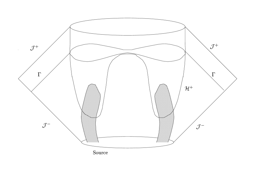
FIG. 1.: The global binary black hole problem involves the event horizon ${\cal H}^{+}$ and future and past null infinity, here approximated by ${\cal J}^{+}$ and ${\cal J}^{-}$. The sources which formed the black holes, e.g. collapsing matter or imploding gravitational waves, are indicated by the shaded regions. The sources are surrounded by a null world tube $\Gamma$, outside of which characteristic evolution supplies the exterior spacetime.

FIG. 2.: The white hole horizon ${\cal H}$ is foliated by an affine parameter $u$, with ${\cal S}^{-}$ representing an early quasi-stationary slice. The affine parameter $\lambda$ along the outgoing null hypersurfaces ${\cal J}_{u}$ emanating from the foliation is chosen so that $\lambda=0$ on ${\cal H}$. The angular coordinates $x^{A}$ are chosen to be constant along the light rays generating ${\cal H}$ and ${\cal J}_{u}$. The null vectors $l^{a}$ and $n^{a}$ are used to project tensor fields into ${\cal H}$.

FIG. 3.: The ingoing null hypersurface normal to an spheroid ${\cal S}_{0}$ in Minkowski space pinches off in the future at points ${\cal X}$, where two null rays cross, bounded by a caustic set ${\cal C}$, where neighboring rays focus; and it expands in the past to a quasi-spherical slice ${\cal S}^{-}$. The foliation by Minkowski time $\hat{t}$ is is shown by horizontal slices. The conformal model induces a white hole affine foliation $u$, indicated by dashed lines, whose upward bulge relative to the Minkowski foliation produces the fission into disjoint white holes depicted in the final $u$-slice shown.

FIG. 4.: The “race” between the minimum values (over the sphere of rays) of the outward expansion and the radius of the horizon, for increasing eccentricities $\epsilon=10^{-7}$ (a), $\epsilon=10^{-6}$ (b), $\epsilon=10^{-5}$ (c), $\epsilon=10^{-4}$ (d), $\epsilon=10^{-3}$ (e), $\epsilon=10^{-2}$ (f), all for mass $M=100$ and $t_{0}=-10$. The expansion is plotted in terms of $\inf(\Theta_{OUT})$ with dashed lines and the radius in terms of $\inf\left(r/(2M)\right)$ with solid lines, both rescaled to unity at the starting time. For small $\epsilon$, the radius hovers near $2M$ longer than it takes the Bondi boundary to form and the fission remains hidden. For larger values of $\epsilon$, the fission occurs before the Bondi boundary, as the sequence shows.

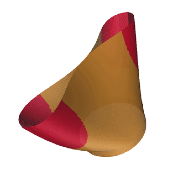
FIG. 5.: Embedding diagram for $\epsilon=10^{-5}$ to depict the shape of the surface, the scales being arbitrary. The darkened region indicates where the outward expansion has gone negative. The expansion first reaches zero at the poles.

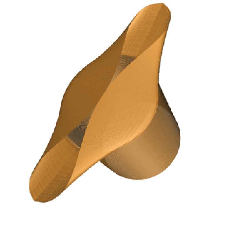
FIG. 6.: Embedding picture for $\epsilon=10^{-3}$. The radius reaches zero first at the equator, at the center of the picture where the individual white holes separate. The expansion is everywhere positive at that time.

FIG. 7.: The radius decreases fastest at the equator, in accord with the trouser-shaped horizon picture.

FIG. 8.: The minimum of the expansion occurs at a pole, hence the expansion wins the race along a polar ray.

FIG. 9.: The curvature scalar ${\cal R}$ of the conformal horizon metric $h_{AB}$ increases from its unit sphere value ${\cal R}=2$ in the region near the poles and decreases in the region near the equator.

FIG. 10.: The behavior of the twist, a quantity which would vanish for the Minkowski time slices of the flat space wave front, shown here for $\epsilon=10^{-5}$.

FIG. 11.: The shear $\sigma_{+,OUT}$ , as depicted in Fig. 11, is positive near the poles and negative near the equator.

REFERENCES

- [1] Luis Lehner, Nigel T. Bishop, Roberto Gómez, Bela Szilágyi, and Jeffrey Winicour, Phys. Rev. D 60, 044005 (1999).
- [2] Sascha Husa and Jeffrey Winicour, Phys. Rev. D 60, 084019 (1999).
- [3] Richard H. Price and Jorge Pullin, Phys. Rev. Lett. 72, 3297 (1994).
- [4] Nigel T. Bishop, Roberto Gómez, Luis Lehner, Manoj Maharaj, and Jeffrey Winicour, Phys. Rev. D 56, 6298 (1997).
- [5] R. Gómez, L. Lehner, R. L. Marsa, and J. Winicour, Phys. Rev. D 57, 4778 (1997).
- [6] J. Winicour, Prog. Theor. Phys. Suppl. 136, 57 (1999).
- [7] Manuela Campanelli, Roberto Gómez, Sascha Husa, Jeffrey Winicour, and Yosef Zlochower, Phys. Rev. D (to be published), gr-qc/0012107.
- [8] H. Bondi, M. van der Burg, and A. Metzner, Proc. R. Soc. London, A269, 21 (1962).
- [9] R. Sachs, Proc. R. Soc. London, A270, 103 (1962).
- [10] R. Sachs, J. Math. Phys. 3, 908 (1962).
- [11] Abhay Ashtekar, Stephen Fairhurst, and Badri Krishnan, Phys. Rev. D 62, 104025 (2000).
- [12] S. A. Hayward, Class. Quantum Grav. 10, 773 (1993).
- [13] S. A. Hayward, Class. Quantum Grav. 10, 779 (1993).
- [14] J. Winicour, J. Math. Phys. 24, 1193 (1983).
- [15] J. Winicour, J. Math. Phys. 25, 2506 (1984).
- [16] R. Gómez, L. Lehner, P. Papadopoulos, and J. Winicour, Class. Quantum Grav. 14, 977 (1997).
- [17] R. Penrose and W. Rindler, Spinors and Space-Time (Cambridge University Press, Cambridge, England, 1984), Vol. 1.
- [18] R. K. Sachs, Proc. R. Soc. London A264, 309 (1961).
- [19] W. Israel, Phys. Rev. 143, 1016 (1966).
- [20] R. Bartnik and A. H. Norton, in Computational Techniques and Applications: CTAC97, edited by B. J. Noye, M. D. Teubner, and A. W. Gill (World Scientific, Singapore, 1998), p. 91.
- [21] R. Bartnik and A. H. Norton, SIAM J. Sci. Comput. (USA) 22, 917 (2000).
- [22] R. Penrose, Phys. Rev. Lett. 14, 57 (1965).
- [23] W. Press, B. Flannery, S. Teukolsky, and W. Vetterling, Numerical Recipes (Cambridge University Press, New York, 1986), Chap. 6.6, p. 182.