WAVEFORMS FOR GRAVITATIONAL RADIATION
FROM COSMIC STRING LOOPS

Abstract

We obtain general formulae for the plus- and cross- polarized waveforms of gravitational radiation emitted by a cosmic string loop in transverse, traceless (synchronous, harmonic) gauge. These equations are then specialized to the case of piecewise linear loops, and it is shown that the general waveform for such a loop is a piecewise linear function. We give several simple examples of the waveforms from such loops. We also discuss the relation between the gravitational radiation by a smooth loop and by a piecewise linear approximation to it.

I INTRODUCTION

Cosmic strings are one dimensional topological defects that may have formed if the vacuum underwent a phase transition at very early times breaking a local $U(1)$ symmetry [1, 2, 3, 4]. The resulting network of strings is of cosmological interest if the strings have a large enough mass per unit length, $\mu$. If $G\mu/c^{2}\sim 10^{-6}$, where $G$ is Newton’s constant and $c$ is the speed of light (i.e. $\mu\sim 10^{22}$g/cm) then cosmic strings may be massive enough to have provided the density perturbations necessary to produce the large scale structure we observe in the Universe today and could explain the pattern of anisotropies observed in the cosmic microwave background [5].

The main constraints on $\mu$ come from observational bounds on the amount of gravitational background radiation emitted by cosmic string loops ([4, 6, 7] and references therein). A loop of cosmic string is formed when two sections of a long string (a string with length greater than the horizon length) meet and intercommute. Once formed, loops begin to oscillate under their own tension, undergoing a process of self-intersection (fragmentation) and eventually creating a family of non-self-intersecting oscillating loops. The gravitational radiation emitted by each loop as it oscillates contributes to the total background gravitational radiation.

In a pair of papers, we introduced and tested a new method for calculating the rates at which energy and momentum are radiated by cosmic strings [8, 9]. Our investigation found that many of the published radiation rates were numerically inaccurate (typically too low by a factor of two). Remarkably, we also found a lower bound (in the center-of-mass frame) for the rate of gravitational radiation from a cosmic string loop [10]. Our method involved the use of piecewise linear cosmic strings. In this paper we wish to provide greater insight into the behaviour of such loops and, in particular, how they approximate smooth loops by examining the waveforms of the gravitational waveforms of such loops.

It has long been known [6, 11] that the first generation of ground-based interferometric gravitational-wave detectors (for example, LIGO-I) will not be able to detect the gravitational-wave stochastic background produced by a network of cosmic strings in the universe. The amplitude of this background is too weak to be detectable, except by a future generation of more advanced instruments. However, a recent paper by Damour and Vilenkin [12] has shown that the non-Gaussian bursts of radiation produced by cusps on the closest loops of strings would be a detectable LIGO-I source. While the specific examples studied here do not include these types of cusps the general method developed can be applied to such loops.

Our space-time conventions follow those of Misner, Thorne and Wheeler [13] so that $\eta_{\mu\nu}=\mathop{\rm diag}(-1,1,1,1)_{\mu\nu}$. We also set $\hbar=c=1$, but we leave $G$ explicit.

II GENERAL THEORY

In the center-of-mass frame, a cosmic string loop is specified by the 3-vector position ${\bf x}(t,\sigma)$ of the string as a function of two variables: time $t$ and a space-like parameter $\sigma$ that runs from $0$ to $L$. (The total energy of the loop is $\mu L$.) When the gravitational back-reaction is neglected, (a good approximation if $G\mu^{2}<\!\!<1$), the string loop satisfies equations of motion whose most general solution in the center-of-mass frame is

$${\bf x}(t,\sigma)={1\over 2}\bigl{[}{\bf a}(u)+{\bf b}(v)\bigr{]}.$$ (1)

where

$$u=t+\sigma,\qquad v=t-\sigma.$$ (2)

Here ${\bf a}(u)\equiv{\bf a}(u+L)$ and ${\bf b}(v)\equiv{\bf b}(v+L)$ are a pair of periodic functions, satisfying the “gauge condition” $|{\bf a}^{\prime}(u)|=|{\bf b}^{\prime}(v)|=1$, where ^′ denotes differentiation with respect to the function’s argument. Because the functions ${\bf a}$ and ${\bf b}$ are periodic in their arguments, the string loop is periodic in time. The period of the loop is $L/2$ since

$${\bf x}(t+{L\over 2},\sigma+{L\over 2})={1\over 2}[{\bf a}(t+\sigma+L)+{\bf b}(t-\sigma)]={1\over 2}[{\bf a}(t+\sigma)+{\bf b}(t-\sigma)]={\bf x}(t,\sigma).$$ (3)

With our choice of coordinates and gauge, the energy-momentum tensor $T^{\mu\nu}$ for the string loop is given by

$$T^{\mu\nu}(t,{\bf y})=\mu\mathop{\int\!\int}\limits_{0\leq u-v\leq 2L}du\,dv\>G^{\mu\nu}(u,v)\delta\bigl{(}t-{\textstyle{1\over 2}}(u+v)\bigr{)}\delta^{(3)}\bigl{(}{\bf y}-{\bf x}(u,v)\bigr{)},$$ (4)

where $G^{\mu\nu}$ is defined by

$$G^{\mu\nu}(u,v)=\partial_{u}x^{\mu}\partial_{v}x^{\nu}+\partial_{v}x^{\mu}\partial_{u}x^{\nu},$$ (5)

with $x^{\mu}=\bigl{(}t,{\bf x}(t,\sigma)\bigr{)}$. In terms of ${\bf a}$ and ${\bf b}$,

$$G^{00}={\textstyle{1\over 2}},\qquad G^{0i}={\textstyle{1\over 4}}[a^{\prime}_{i}+b^{\prime}_{i}],\qquad G^{ij}={\textstyle{1\over 4}}[a^{\prime}_{i}b^{\prime}_{j}+a^{\prime}_{j}b^{\prime}_{i}],$$ (6)

and the trace is

$$G^{\lambda}{}_{\lambda}={\textstyle{1\over 2}}[-1+{\bf a}^{\prime}{\cdot}{\bf b}^{\prime}].$$ (7)

Alternatively we may introduce the four-vectors $A^{\mu}(u)=\bigl{(}u,{\bf a}(u)\bigr{)}$ and $B^{\mu}(v)=\bigl{(}v,{\bf b}(v)\bigr{)}$ so that

$$G^{\mu\nu}={\textstyle{1\over 4}}(A^{\prime}{}^{\mu}B^{\prime}{}^{\nu}+B^{\prime}{}^{\mu}A^{\prime}{}^{\nu}).$$ (8)

The “gauge conditions” are satisfied if and only if $A^{\prime}{}^{\mu}(u)$ and $B^{\prime}{}^{\mu}(v)$ are null vectors.

As a consequence of the time periodicity of the loop the stress tensor can be expressed as a Fourier series

$$T_{\mu\nu}(t,{\bf y})=\sum\limits_{n=-\infty}^{\infty}\>e^{i\omega_{n}t}\>\tilde{T}_{\mu\nu}(\omega_{n},{\bf y}),$$ (9)

where $\omega_{n}=4\pi n/L$ and

$$\tilde{T}_{\mu\nu}(\omega_{n},{\bf y}) = {2\over L}\int\limits_{0}^{L/2}{\rm d}t\>e^{-i\omega_{n}t}T_{\mu\nu}(t,{\bf y})$$ (10)

$$= {2\mu\over L}\int\limits_{0}^{L}du\int\limits_{0}^{L}dv\>e^{-{1\over 2}i\omega_{n}(u+v)}G^{\mu\nu}(u,v)\delta^{(3)}\bigl{(}{\bf y}-{\bf x}(u,v)\bigr{)}.$$ (11)

The retarded solution for the linear metric perturbation due to this source in harmonic gauge is [14]

$$h_{\mu\nu}(t,{\bf x})=4G\sum\limits_{n=-\infty}^{\infty}\int{d^{3}{\bf y}\over|{\bf x}-{\bf y}|}\>\Bigl{[}\tilde{T}_{\mu\nu}(\omega_{n},{\bf y})-{\textstyle{1\over 2}}\eta_{\mu\nu}\tilde{T}^{\lambda}{}_{\lambda}(\omega_{n},{\bf y})\Bigr{]}\,e^{i\omega_{n}(t-|{\bf x}-{\bf y}|)}.$$ (12)

Far from the string loop center-of-mass the dominant behavior is that of an outgoing spherical wave given by

$$h_{\mu\nu}(t,{\bf x})=4G\sum\limits_{n=-\infty}^{\infty}{e^{i\omega_{n}(t-r)}\over r}\int d^{3}{\bf y}\>\Bigl{[}\tilde{T}_{\mu\nu}(\omega_{n},{\bf y})-{\textstyle{1\over 2}}\eta_{\mu\nu}\tilde{T}^{\lambda}{}_{\lambda}(\omega_{n},{\bf y})\Bigr{]}\,e^{i\omega_{n}\hat{\bf\Omega}{\cdot}{\bf y}},$$ (13)

where $r=|x|$ and $\hat{\bf\Omega}={\bf x}/r$ is a unit vector pointing away from the source. Inserting Eq. (11) into Eq. (13) we find the field far from a cosmic string loop is

$$h_{\mu\nu}(t,{\bf x})={8G\mu\over L}\sum\limits_{n=-\infty}^{\infty}{e^{i\omega_{n}(t-r)}\over r}\int\limits_{0}^{L}du\int\limits_{0}^{L}dv\>\Bigl{[}\tilde{G}_{\mu\nu}(u,v)-{\textstyle{1\over 2}}\eta_{\mu\nu}\tilde{G}^{\lambda}{}_{\lambda}(u,v)\Bigr{]}\,e^{-i\omega_{n}\bigl{[}{1\over 2}(u+v)-\hat{\bf\Omega}{\cdot}{\bf x}(u,v)\bigr{]}}.$$ (14)

The $n=0$ term in this sum corresponds to the static field

$$h^{\rm static}_{\mu\nu}(t,{\bf x})={8G\mu\over rL}\int\limits_{0}^{L}{\rm d}u\int\limits_{0}^{L}{\rm d}v\>\Bigl{[}G_{\mu\nu}(u,v)-{\textstyle{1\over 2}}\eta_{\mu\nu}G^{\lambda}{}_{\lambda}(u,v)\Bigr{]},$$ (15)

$$={2G\mu L\over r}(\eta_{\mu\nu}+2\hat{t}_{\mu}\hat{t}_{\nu})={2GM\over r}\delta_{\mu\nu},$$ (16)

as appropriate to a object with mass $M$ as may be seen by comparison with the Schwarzschild metric in isotropic coordinates (see, for example, Eq. (31.22) of Ref. [13]). We denote the radiative part of the field by

$$h^{\rm rad}_{\mu\nu}=h_{\mu\nu}-h^{\rm static}_{\mu\nu}.$$ (17)

We may rewrite Eq. (14) as

$$h_{\mu\nu}(t,{\bf x})=\sum\limits_{n=-\infty}^{\infty}e^{-i\omega_{n}k_{\mu}x^{\mu}}{\rm e}^{(n)}{}_{\mu\nu}(\hat{\bf\Omega})$$ (18)

where $k^{\mu}=(1,\hat{\bf\Omega})$ is a null vector in the direction of propagation and

$${\rm e}^{(n)}{}_{\mu\nu}={8GM\over rL^{2}}\int\limits_{0}^{L}du\int\limits_{0}^{L}dv\>\Bigl{[}G_{\mu\nu}(u,v)-{\textstyle{1\over 2}}\eta_{\mu\nu}G^{\lambda}{}_{\lambda}(u,v)\Bigr{]}\,e^{i{1\over 2}\omega_{n}\bigl{[}k_{\mu}A^{\mu}(u)+k_{\mu}B^{\mu}(v)\bigr{]}}$$ (19)

are polarization tensors. From Eq. (8), it is clear that the polarization tensors may be written in terms of the fundamental integrals

$$I^{(n)}{}^{\mu}={1\over L}\int\limits_{0}^{L}du\>A^{\prime}{}^{\mu}(u)\,e^{i{1\over 2}\omega_{n}k_{\mu}A^{\mu}(u)},$$ (20)

and

$$J^{(n)}{}^{\mu}={1\over L}\int\limits_{0}^{L}dv\>B^{\prime}{}^{\mu}(v)\,e^{i{1\over 2}\omega_{n}k_{\mu}B^{\mu}(v)}.$$ (21)

In terms of these integrals

$${\rm e}_{00}={2GM\over r}\left[I_{0}J_{0}+{\bf I}{\cdot}{\bf J}\right]$$ (23)

$${\rm e}_{0i}={2GM\over r}\left[I_{0}J_{i}+J_{0}I_{i}\right]$$ (24)

$${\rm e}_{ij}={2GM\over r}\left\{\left[I_{i}J_{j}+J_{i}I_{j}\right]+\delta_{ij}\left[I_{0}J_{0}-{\bf I}{\cdot}{\bf J}\right]\right\},$$ (25)

where we have dropped the superscript $(n)$ for clarity.

The harmonic gauge condition requires that the polarization tensors satisfy $k^{\mu}{\rm e}_{\mu\nu}={1\over 2}k_{\nu}{\rm e}_{\mu}{}^{\mu}$. This is easily verified by noting that $I^{0}=\hat{\bf\Omega}{\cdot}{\bf I}$ and $J^{0}=\hat{\bf\Omega}{\cdot}{\bf J}$. These equations follow from the identity

$$\int\limits_{0}^{L}du\>k_{\mu}A^{\prime}{}^{\mu}(u)\,e^{-i{1\over 2}\omega_{n}k_{\nu}A^{\nu}(u)}={2i\over\omega}\int\limits_{0}^{L}du\>{d\ \over du}\,e^{-i{1\over 2}\omega_{n}k_{\nu}A^{\nu}(u)}=0,$$ (26)

which is a consequence of periodicity, and the corresponding equation for $B^{\mu}$. The harmonic gauge condition does not determine the gauge completely and we are left with the freedom to make transformations of the form

$${\rm e}^{\prime}{}_{\mu\nu}={\rm e}_{\mu\nu}+k_{\mu}\varepsilon_{\nu}+k_{\nu}\varepsilon_{\mu}.$$ (27)

If we make the choice

$$\varepsilon_{0}={GM\over r}\left[I_{0}J_{0}+{\bf I}{\cdot}{\bf J}\right]$$ (29)

and

$$\varepsilon_{i}={GM\over r}\left\{\left[I_{0}J_{0}+{\bf I}{\cdot}{\bf J}\right]\Omega_{i}+2\left[I_{0}J_{i}+J_{0}I_{i}\right]\right\}$$ (30)

then

$${\rm e}^{\prime}{}_{0\mu}=0.$$ (31)

The spatial components are given by

$${\rm e}^{\prime}{}_{ij}={2GM\over r}\bigl{\{}[I_{i}J_{j}+I_{j}J_{i}]+\delta_{ij}[I_{0}J_{0} - {\bf I}{\cdot}{\bf J}]+\Omega_{i}\Omega_{j}[I_{0}J_{0}+{\bf I}{\cdot}{\bf J}]$$ (32)

$$+ I_{0}[J_{i}\Omega_{j}+\Omega_{i}J_{j}]+J_{0}[I_{i}\Omega_{j}+\Omega_{i}I_{j}]\bigr{\}},$$ (33)

these satisfy the gauge conditions

$${\rm e}^{\prime}{}_{\mu}{}^{\mu}={\rm e}^{\prime}{}_{i}{}^{i}=0,$$ (34)

and

$${\rm e}^{\prime}{}_{j}{}^{i}\Omega_{i}=0.$$ (35)

If we perform a spatial rotation to coordinates $(x^{\prime},y^{\prime},z^{\prime})$ where $\hat{\bf\Omega}$ points along the $z^{\prime}$-axis then we can write

$${\rm e}^{\prime}{}_{i^{\prime}j^{\prime}}=\left(\matrix{e_{+}&e_{\times}&0\cr e_{\times}&-e_{+}&0\cr 0&0&0}\right),$$ (36)

where

$$e_{+}={2GM\over r}[I_{1^{\prime}}J_{1^{\prime}}-I_{2^{\prime}}J_{2^{\prime}}]$$ (38)

and

$$e_{\times}={2GM\over r}[I_{1^{\prime}}J_{2^{\prime}}+I_{2^{\prime}}J_{1^{\prime}}],$$ (39)

define two modes of linear polarization.

In terms of the original basis we can write

$$e_{+}={2GM\over r}(\cos 2\psi A_{+}+\sin 2\psi A_{\times})$$ (41)

and

$$e_{\times}={2GM\over r}(-\sin 2\psi A_{+}+\cos 2\psi A_{\times})$$ (42)

with

$$A_{+}= \Bigl{\{}(\cos^{2}\theta\cos^{2}\phi-\sin^{2}\phi)I_{1}J_{1}+(\cos^{2}\theta\sin^{2}\phi-\cos^{2}\phi)I_{2}J_{2}+\sin^{2}\theta I_{3}J_{3}$$ (46)

$$+(1+\cos^{2}\theta)\cos\phi\sin\phi(I_{2}J_{1}+I_{1}J_{2})-\sin\theta\cos\theta\cos\phi(I_{3}J_{1}+I_{1}J_{3})$$

$$-\sin\theta\cos\theta\sin\phi(I_{2}J_{3}+I_{3}J_{2})\Bigr{\}}$$

$$A_{\times}= \Bigl{\{}-2\cos\theta\sin\phi\cos\phi I_{1}J_{1}+2\cos\theta\sin\phi\cos\phi I_{2}J_{2}+\cos\theta(2\cos^{2}\phi-1)(I_{2}J_{1}+I_{1}J_{2})$$ (48)

$$+\sin\theta\sin\phi(I_{3}J_{1}+I_{1}J_{3})-\sin\theta\cos\phi(I_{2}J_{3}+I_{3}J_{2})\Bigr{\}}$$

where $\theta$, $\phi$ and $\psi$ are the Euler angles defining the orientation of the frame $(x^{\prime},y^{\prime},z^{\prime})$ relative to the original frame (our conventions follow those of Ref. [15]). The corresponding linearly polarized waveforms are then defined by

$$h^{\rm rad}_{+/\times}(t,{\bf x})=\sum\limits_{n=1}^{\infty}\Bigl{\{}e^{i4\pi n(t-r)/L}{\rm e}^{(n)}_{+/\times}+e^{-i4\pi n(t-r)/L}{\rm e}^{(n)*}_{+/\times}\Bigr{\}}.$$ (49)

Recall that $h^{\rm rad}$ is obtained from the full metric perturbation $h$ by dropping the $n=0$ term which corresponds to the static (non-radiative) part of the field.

The power emitted to infinity per solid angle may be written as

$${dP\over d\Omega} = \lim_{r\to\infty}{r^{2}\over 32\pi G}\langle h_{\alpha\beta,t}h^{\alpha\beta}{}_{,r}\rangle$$ (50)

$$= {GM^{2}\over 2\pi}\sum\limits_{n=1}^{\infty}\omega_{n}^{2}\bigl{\{}\langle|A_{+}^{(n)}|^{2}\rangle+\langle|A_{\times}^{(n)}|^{2}\rangle\bigr{\}}.$$ (51)

III EXAMPLES

For convenience we shall now set the length of the loop $L=1$, and take $\psi=0$.

A Piecewise linear loops

These are loops for which the functions ${\bf a}(u)$ and ${\bf b}(v)$ are piecewise linear functions. The functions ${\bf a}(u)$ and ${\bf b}(v)$ may be pictured as a pair of closed loops which consist of joined straight segments. The segments join together at kinks where ${\bf a}^{\prime}(u)$ and ${\bf b}^{\prime}(v)$ are discontinuous.

Following the notation of Ref. [8] we take the $a$- and $b$-loops to have $N_{a}$ and $N_{b}$ linear segments, respectively. The coordinate $u$ on the $a$-loop is chosen to take the value zero at one of the kinks and increases along the loop. The kinks are labeled by the index $i$ where $i=0,1,\dots,N_{a}-1$. The value of $u$ at the $i$th kink is denoted by $u_{i}$ and without loss of generality we set $u_{0}=0$. The segments on the loop are also labeled by $i$, with the $i$th segment being the one lying between the $i$th and $(i+1)$th kink. The kink at $u=u_{N_{a}}$ is the same as the first kink at $u=u_{0}=0$ but, even though $u_{0}$ and $u_{N_{a}}$ are at the same position on the loop, $u_{0}=0$ while $u_{N_{a}}=1$. The loop is extended to all values of $u$ by periodicity (with period 1). We denote ${\bf a}_{i}={\bf a}(u_{i})$, and the constant unit vector tangent to the $i$th segment by ${\bf a}^{\prime}_{i}$. Then we have

$${\bf a}(u)={\bf a}_{i}+{\bf a}_{i}^{\prime}(u-u_{i})\qquad\hbox{for \ }u\in[u_{i},u_{i+1}],$$ (52)

and for consistency

$${\bf a}_{i+1}={\bf a}_{i}+{\bf a}_{i}^{\prime}(u_{i+1}-u_{i}).$$ (53)

We have corresponding definitions for the ${\bf b}$-loop and we follow the convention of Ref. [8] by labeling the kinks by the index $j$.

It is now elementary to calculate that, for $n\neq 0$,

$${\bf I}^{(n)} = {1\over 2\pi in}\sum\limits_{i=0}^{N_{a}-1}{{\bf a}_{i}^{\prime}\over 1-\hat{\bf\Omega}{\cdot}{\bf a}_{i}^{\prime}}\left\{e^{-2\pi in(u_{i+1}-\hat{\bf\Omega}{\cdot}{\bf a}_{i+1})}-e^{-2\pi in(u_{i}-\hat{\bf\Omega}{\cdot}{\bf a}_{i})}\right\}$$ (54)

$$= {i\over 2\pi n}\sum\limits_{i=0}^{N_{a}-1}\left\{{{\bf a}_{i}^{\prime}\over 1-\hat{\bf\Omega}{\cdot}{\bf a}_{i}^{\prime}}-{{\bf a}_{i-1}^{\prime}\over 1-\hat{\bf\Omega}{\cdot}{\bf a}_{i-1}^{\prime}}\right\}e^{-2\pi in(u_{i}-\hat{\bf\Omega}{\cdot}{\bf a}_{i})},$$ (55)

with a similar equation for ${\bf J}$. If we insert these expressions into Eq. (II) and then into Eq. (49) the sum over $n$ for $h_{R/L}^{\rm rad}$ consists of terms of the form

$$\sum_{n=1}^{\infty}{1\over n^{2}}\cos{2\pi n[2(t-r)+(u_{i}-\hat{\bf\Omega}{\cdot}{\bf a}_{i})+(v_{j}-\hat{\bf\Omega}{\cdot}{\bf b}_{j})]}$$ (56)

which may be performed exactly using the identity

$$\sum_{n=1}^{\infty}{1\over n^{2}}\cos{2\pi nx}=\pi^{2}(x^{2}-x+{\textstyle{1\over 6}})\qquad x\in[0,1).$$ (57)

This function is extended to other values by periodicity, for example, for $x\in[1,2)$ we merely replace $x$ by $x-1$ in Eq. (57). Such transformations leave the coefficient of $x^{2}$ unchanged and can only change the coefficient of $x$ by a multiple of 2. As a result when the sum in Eq. (55) is performed for the coefficient of $x^{2}$ the sum telescopes and gives zero. Thus, the waveform of a piecewise linear loop will be a piecewise linear function. In addition, considering the coefficient of $x$ all slopes of the waveform must be a multiple of some fundamental slope. The slope only changes when a (4-dimensional) kink crosses the past light cone of the observer at $(t,{\bf x})$. These properties are illustrated in the examples below.

B Garfinkle-Vachaspati loops

As our first set of loops we study the loops considered by Garfinkle and Vachaspati [16]. The vectors ${\bf a}(u)$ and ${\bf b}(v)$ lie in a plane and make a constant angle $2\alpha$ with each other where $\alpha\in(0,\pi/2)$. To be specific, we may take ${\bf a}(u)$ and ${\bf b}(v)$ to be given by

$${\bf a}(u)=\cases{u(\cos\alpha{\bf i}+\sin\alpha{\bf j}),&$u\in(0,{1\over 2})$\cr&\cr(1-u)(\cos\alpha{\bf i}+\sin\alpha{\bf j}),&$u\in({1\over 2},1)$}$$ (59)

$${\bf b}(v)=\cases{v(\cos\alpha{\bf i}-\sin\alpha{\bf j}),&$v\in(0,{1\over 2})$\cr&\cr(1-v)(\cos\alpha{\bf i}-\sin\alpha{\bf j}),&$v\in({1\over 2},1)$.}$$ (60)

It is then straightforward to calculate that, for $n\neq 0$,

$${\bf I}^{(n)} = {e^{i\pi n\bigl{(}1-\sin\theta\cos(\phi-\alpha)\bigr{)}}-1\over i\pi n\bigl{(}1-\sin^{2}\theta\cos^{2}(\phi-\alpha)\bigr{)}}(\cos\alpha{\bf i}+\sin\alpha{\bf j})$$ (62)

$${\bf J}^{(n)} = {e^{i\pi n\bigl{(}1-\sin\theta\cos(\phi+\alpha)\bigr{)}}-1\over i\pi n\bigl{(}1-\sin^{2}\theta\cos^{2}(\phi+\alpha)\bigr{)}}(\cos\alpha{\bf i}-\sin\alpha{\bf j})$$ (63)

and correspondingly

$$A_{+}^{(n)} = {\sin^{2}\theta\cos(\phi+\alpha)\cos(\phi-\alpha)-\cos 2\phi\over\bigl{(}1-\sin^{2}\theta\cos^{2}(\phi-\alpha)\bigr{)}\bigl{(}1-\sin^{2}\theta\cos^{2}(\phi+\alpha)\bigr{)}}\times$$ (66)

$${1\over n^{2}\pi^{2}}(e^{i\pi n\bigl{(}1-\sin\theta\cos(\phi-\alpha)\bigr{)}}-1)(e^{i\pi n\bigl{(}1-\sin\theta\cos(\phi+\alpha)\bigr{)}}-1)$$

$$A_{\times}^{(n)} = {\cos\theta\sin 2\phi\over\bigl{(}1-\sin^{2}\theta\cos^{2}(\phi-\alpha)\bigr{)}\bigl{(}1-\sin^{2}\theta\cos^{2}(\phi+\alpha)\bigr{)}}\times$$ (68)

$${1\over n^{2}\pi^{2}}(e^{i\pi n\bigl{(}1-\sin\theta\cos(\phi-\alpha)\bigr{)}}-1)(e^{i\pi n\bigl{(}1-\sin\theta\cos(\phi+\alpha)\bigr{)}}-1).$$

As described above, the sum over $n$ in Eq. (49) may be performed explicitly to yield a piecewise linear function. For example, $\phi\in[0,\pi/2)$, $h_{+}$ is given explicitly by

$$h_{+} ={2GM\over r}{\sin^{2}\theta\cos(\phi+\alpha)\cos(\phi-\alpha)-\cos 2\phi\over\bigl{(}1-\sin^{2}\theta\cos^{2}(\phi-\alpha)\bigr{)}\bigl{(}1-\sin^{2}\theta\cos^{2}(\phi+\alpha)\bigr{)}}\times$$ (70)

$$\cases{(1-\sin\theta\cos(\phi-\alpha))(1-\sin\theta\cos(\phi+\alpha)),&\cr\qquad\hfill 0\leq(t-r)<{\textstyle{1\over 4}}\sin\theta\bigl{(}\cos(\phi-\alpha)+\cos(\phi+\alpha)\bigr{)}&\cr&\cr-8(t-r)+(1+\sin\theta\cos(\phi+\alpha))(1+\sin\theta\cos(\phi-\alpha)),&\cr\qquad\hfill{\textstyle{1\over 4}}\sin\theta\bigl{(}\cos(\phi-\alpha)+\cos(\phi+\alpha)\bigr{)}\leq(t-r)<{\textstyle{1\over 4}}(1+\sin\theta\cos(\phi+\alpha))&\cr&\cr-(1-\sin\theta\cos(\phi-\alpha))(1+\sin\theta\cos(\phi+\alpha)),&\cr\qquad\hfill{\textstyle{1\over 4}}(1+\sin\theta\cos(\phi+\alpha))\leq(t-r)<{\textstyle{1\over 4}}(1+\sin\theta\cos(\phi-\alpha))&\cr&\cr 8(t-r-{\textstyle{1\over 2}})+(1-\sin\theta\cos(\phi-\alpha))(1-\sin\theta\cos(\phi+\alpha)),&\cr\qquad\hfill{\textstyle{1\over 4}}(1+\sin\theta\cos(\phi-\alpha))\leq(t-r)<{\textstyle{1\over 2}}.&\cr}$$

and the waveforms are periodic in $t$ with period $1\over 2$. The intervals are ordered in the given way for our choice of $\phi\in[0,\pi/2)$. $h_{\times}$ is obtained simply by replacing the prefactor by that appropriate to $A_{\times}$ as is clear from Eq. (III B). To obtain the waveforms for other angles we may note that the transformation $\phi\to\phi+\pi$ is equivalent to changing the sign of $(t-r)$, while the transformation $\phi\to\pi-\phi$ is equivalent to changing the sign of $(t-r)$ and sign in front of the $\sin 2\phi$ term in the prefactor in $h_{\times}$.

Note that the apparent singularity in the waveforms in the plane of the loop ($\theta=\pi/2$) at $\phi=\pm\alpha$ and $\phi=\pi\pm\alpha$ is spurious. This may be seen by noting that the waveform is bounded by the two constant sections of the piecewise linear curve which take on a value which tends to zero in this limit. In fact, the numerator of the prefactor also vanishes in this limit which ensures that the amplitude tends to zero at these points and hence that even the time derivatives (which determine the power) are finite. Along the axis $\theta=0$, Eq. (LABEL:gv_waveform) reduces to

$$h_{+/\times}(\theta=0)=-{2GM\over r}\cos 2\phi/\sin{2\phi}\cases{-8(t-r)+1,&$0\leq t-r<{\textstyle{1\over 4}}$\cr&\cr 8(t-r-{\textstyle{1\over 2}})+1,&${\textstyle{1\over 4}}\leq t-r<{\textstyle{1\over 2}}$.}$$ (72)

Waveforms for various angles a plotted in Fig. 1 for the case of $\alpha=\pi/4$, corresponding to two lines at right angles. This is the configuration which radiates minimum gravitational radiation for this class of loops, $P=64\ln 2\>G\mu^{2}\approx 44{\cdot}3614\>G\mu^{2}$.

C Plane-line loops

As our next set of examples we study the set of loops in which ${\bf a}(u)$ lies along the $z$-axis and ${\bf b}(v)$ is always in the $x$-$y$ plane. This class of loops was studied by us in Ref. [17] where we gave an analytic result for the power lost in gravitational radiation by such loops. Explicitly ${\bf a}(u)$ is given by

$${\bf a}(u)=\cases{u{\bf k}&$u\in(0,{1\over 2})$\cr&\cr(1-u){\bf k}&$u\in({1\over 2},1)$.}$$ (73)

It follows that

$${\bf I}^{(n)}={e^{i\pi n(1-\cos\theta)}-1\over i\pi n\sin^{2}\theta}{\bf k}.$$ (74)

Also $J^{(n)}_{3}=0$, so we have

$$A_{+} = -\sin\theta\cos\theta(\cos\phi J_{1}+\sin\phi J_{2})I_{3}$$ (76)

$$A_{\times} = \sin\theta(\sin\phi J_{1}-\cos\phi J_{2})I_{3}.$$ (77)

It follows immediately that the waveforms vanish along the $z$-axis.

In Ref. [17] we proved that the minimum gravitational radiation emitted by any loop in this class is given by taking the ${\bf b}$-loop to be a circle:

$${\bf b}(v)={1\over 2\pi}\bigl{(}\cos(2\pi v){\bf i}+\sin(2\pi v){\bf j}\bigr{)}.$$ (78)

The power emitted in gravitational radiation by this loop is

$$P=16\int\limits_{0}^{2\pi}{(1-\cos x)\over x}\,dx\>G\mu^{2}\approx 39{\cdot}0025\>G\mu^{2}.$$ (79)

${\bf J}^{(n)}$ may be determined explicitly as

$$J^{(n)}_{1} = {i\over 2}\left[e^{i(n+1)(\phi-{\pi\over 2})}J_{n+1}(n\sin\theta)-e^{i(n-1)(\phi-{\pi\over 2})}J_{n-1}(n\sin\theta)\right]$$ (81)

$$J^{(n)}_{2} = {1\over 2}\left[e^{i(n+1)(\phi-{\pi\over 2})}J_{n+1}(n\sin\theta)+e^{i(n-1)(\phi-{\pi\over 2})}J_{n-1}(n\sin\theta)\right]$$ (82)

This gives the equivalent forms

$$A_{+}^{(n)} = -{\sin\bigl{(}\pi n\sin^{2}(\theta/2)\bigr{)}\cos\theta\over\sin\theta}\left[J_{n+1}(n\sin\theta)+J_{n-1}(n\sin\theta)\right]{1\over\pi n}e^{i\pi n\sin^{2}(\theta/2)+in(\phi-\pi/2)}$$ (83)

$$= -2{\sin\bigl{(}\pi n\sin^{2}(\theta/2)\bigr{)}\cos(\theta)\over\sin^{2}\theta}J_{n}(n\sin\theta){1\over\pi n}e^{in\phi-in(\pi/2)\cos\theta}.$$ (84)

and

$$A_{\times}^{(n)} = i{\sin\bigl{(}\pi n\sin^{2}(\theta/2)\bigr{)}\over\sin\theta}\left[J_{n+1}(n\sin\theta)-J_{n-1}(n\sin\theta)\right]{1\over\pi n}e^{i\pi n\sin^{2}(\theta/2)+in(\phi-\pi/2)}$$ (85)

$$= 2i{\sin\bigl{(}\pi n\sin^{2}(\theta/2)\bigr{)}\over\sin\theta}J_{n}^{\prime}(n\sin\theta){1\over\pi n}e^{in\phi-in(\pi/2)\cos\theta}.$$ (86)

The corresponding waveforms for various choices of $\theta$ are plotted in Figs. 2 and 3. (As the system simply rotates cylindrically with time the choice of $\phi$ is irrelevant, corresponding simply to a shift in $t-r$.)

In the plane of the ${\bf b}$-loop $h_{+}$ vanishes so that the wave becomes linearly polarized. On the other hand, as we approach the axis $\theta=0$ the fundamental mode ($n=1$ term) dominates and we have

$$h_{+}\sim-{GM\over r}\sin\theta\sin\bigl{(}4\pi(t-r)+\phi\bigr{)}$$ (87)

and

$$h_{\times}\sim{GM\over r}\sin\theta\cos\bigl{(}4\pi(t-r)+\phi\bigr{)}.$$ (88)

Thus the wave approaches circular polarization but its amplitude vanishes as $\sin\theta$.

As in Ref. [17] we may also consider the case where the ${\bf b}$-loop forms a regular $N$-sided polygon. In Figs. 4 and 5 we compare the waveform for the circle with that for a regular hexagon for which $P=(40\ln 5-32\ln 2)\>G\mu^{2}\approx 42{\cdot}1968\>G\mu^{2}$. As mentioned above a change in $\phi$ for the circle-line loop corresponds simply to a shift in $t$, however, this is no longer the case for the polygon for which the waveform will only repeat every $2\pi/N$. Hence in Figs. 4 and 5 we include hexagon-line waveform for both $\phi=0$ and $\phi=5\pi/6$ (this choice was made simply to disentangle the two graphs as far as possible). It is remarkable that even for such a crude approximation to the circle as a hexagon, the waveform of the hexagon-line loop provides remarkably good piecewise linear approximations to the circle-line waveforms.

IV CONCLUSION

Given the remarkable agreement of the waveforms it is of interest to compare the ‘instantaneous power’ defined by

$$P_{+/\times}={GM^{2}\over 2\pi}\sum\limits_{n=1}^{\infty}\omega_{n}^{2}|A_{+/\times}^{(n)}|^{2}$$ (89)

in the different polarizations. While this quantity is not gauge invariant its time average is and gives the total power radiated in each polarization. By comparing the function for the polygon-line loops with the circle-line loop we can certainly see that their time averages agree well. As the waveform for a piecewise linear loop is a piecewise linear function, the instantaneous power, which is the square of its derivative, will be piecewise constant. For example, in Fig. 6 we compare the ‘instantaneous power’ in the plus-polarization between the circle-line loop and a regular 24-sided polygon-line loop. The very close agreement between the two curves provides further evidence for the validity of the piecewise linear approximation of string loops used by [8].

FIG. 1.: Plus-polarized waveforms for the Garfinkle-Vachaspati with $\alpha=\pi/4$. The solid line corresponds to the wave travelling up the $z$-axis ($\theta=0$). The dotted line corresponds to a direction at elevation $\theta=\pi/3$ along $\phi=0$. The dashed line corresponds to a wave travelling in the plane of the loop $\theta=\pi/2$) at angle $\phi=\pi/5$. The cross-polarized waveforms differ only in that there amplitude has a different dependece on $\theta$ and $\phi$.

FIG. 2.: Plus-polarized waveforms for the circle-line loop. Plotted is $h_{+}/\sin\theta$ for $\theta=\pi/2$ (solid), $\theta=\pi/4$ (dashed) and $\theta=\pi/20$ (dotted). The choice of scaling is chosen on the basis of the asymptotic form Eq. (87).

FIG. 3.: Cross-polarized waveforms for the circle-line loop. Plotted is $h_{\times}/\sin\theta$ for $\theta=\pi/2$ (solid), $\theta=\pi/4$ (dashed) and $\theta=\pi/20$ (dotted). The choice of scaling is chosen on the basis of the asymptotic form Eq. (88).

FIG. 4.: The solid lines are the plus-polarized waveforms for the hexagon-line loop with $\theta=\pi/4$ and with $\phi=0$ (left through) and $\phi=5\pi/6$ (right through). The dotted lines are the corresponding waveforms for the circle-line loop.

FIG. 5.: The solid lines are the cross-polarized waveforms for the hexagon-line loop with $\theta=\pi/4$ and with $\phi=0$ (left peak) and $\phi=5\pi/6$ (right peak). The dotted lines are the corresponding waveforms for the circle-line loop.

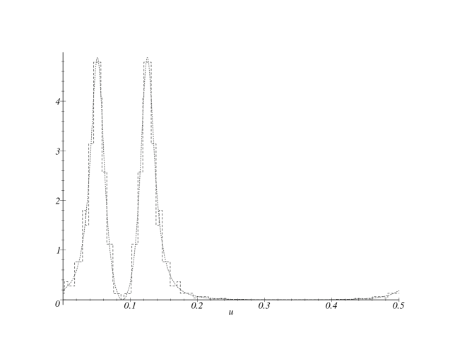
FIG. 6.: Comparison of the ‘instantaneous power’ in plus-polarized waves for the 24-sided polygon-line loop (dotted line) and for the circle-line loop (solid line) with $\theta=\pi/4$ and $\phi=0$.

REFERENCES

• [1] T. W. B. Kibble, J. Phys. A 9, 1387 (1976); T. W. B. Kibble, G. Lazarides, and Q. Shafi, Phys. Rev. D 26, 435 (1982).
• [2] Y. B. Zel’dovich, Mon. Not. R. Astron. Soc. 192, 663 (1980).
• [3] A. Vilenkin, Phys. Rev. D 24, 2082 (1981); Phys. Rep. 121, 263 (1985).
• [4] E.P.S. Shellard and A. Vilenkin, Cosmic Strings and other Topological Defects, (Cambridge University Press, Cambridge, England, 1994).
• [5] B. Allen, R.R. Caldwell, E.P.S. Shellard, A. Stebbins, S. Veeraraghavan, Phys.Rev.Lett. 77, 3061 (1996).
• [6] B. Allen and R.R. Caldwell, Phys. Rev. D 45, 3447 (1992).
• [7] R.R. Caldwell, “Current observational constraints on cosmic strings”, in Proceedings of the Fifth Canadian General Relativity and Gravitation Conference, 1993, ed. R. McLenaghan and R. Mann (World Scientific, New York, 1993).
• [8] B. Allen and P. Casper, Phys. Rev. D 50, 2496 (1994).
• [9] B. Allen, P. Casper, and A. Ottewill, Phys. Rev. D 51, 1546 (1995).
• [10] B. Allen and P. Casper, Phys. Rev. D 52, 4337 (1995).
• [11] B. Allen, The stochastic gravity-wave background: sources and detection, in Proceedings of the Les Houches School on Astrophysical Sources of Gravitational Radiation, eds. J.A. Marck and J.P. Lasota, (Cambridge University Press, Cambridge, England, 1997).
• [12] T. Damour and A. Vilenkin, Gravitational wave bursts from cosmic strings, gr-qc/0004075
• [13] C. W. Misner, K. S. Thorne and J. A. Wheeler, Gravitation (Freeman, San Francisco, 1973).
• [14] S. Weinberg, Gravitation and Cosmology, (John Wiley, New York,1972).
• [15] G. Arfken, Mathematical methods for physicists, third edition, (Academic Press, Orlando, 1985).
• [16] D. Garfinkle and T. Vachaspati, Phys. Rev. D 36, 2229 (1987).
• [17] B. Allen, P. Casper, and A. Ottewill, Phys. Rev. D 50, 3703 (1994).
Refer to caption