Constructing stellar objects with multiple necks

1 Introduction

The theory of static spherically symmetric (SSS) relativistic stellar models has received an increasing interest in recent years. A few years ago Chandrasekhar and Ferrari [1] discovered the phenomenon of trapped gravitational waves in ultracompact objects. Later Abramowicz et al. [2] showed that the trapping could be conveniently visualized in terms of the optical geometry of the models. It follows from their work that trapping occurs when the optical geometry has a sufficiently pronounced neck. The physical relevance of the neck stems from the fact that it is associated with an unstable closed lightlike circular orbit. This phenomenon is present in the exterior Schwarzschild geometry at $R=3M$ as is well-known. Any SSS stellar object which is more compact than $R=3M$ will therefore have a neck. However, Rosquist showed in [3] that the limit $R\lesssim 3M$ is not essential for the formation of a neck and hence it is not essential for a trapping region either. In particular, a neck can exist in the stellar interior. Because the optical geometry is regular all the way down to the center of the star, a neck is always associated with a bulge which is located further inside the stellar interior. Moreover, as was pointed out in [4], there exist models with multiple necks. In fact the number of necks can be unbounded for a given equation of state. Some examples of double neck models with quite pronounced double necks were given in [5]. In the present paper we show how such models can be constructed. We also prove the statements made in [4].

The relation between necks and the optical geometry can be described in terms of the centrifugal potential ($V_{l}$) which governs the null geodesic orbits in the stellar spacetime. A slight modification ($V=V_{l}+V_{m}$) of this potential is responsible for the propagation of axial gravitational wave modes. In this picture a bulge corresponds to a potential well in which trapped modes may exist. Models with multiple necks (and hence bulges) have potentials with multiple wells. The corresponding gravitational wave modes can therefore be considerably more complicated than the single well modes.

Our analysis relies on a recent dynamical systems approach by Nilsson and Uggla [6, 7] who treated the full solution space of the SSS field equations, with focus on the case of linear and polytropic equation of state. Nilsson and Uggla give three different dynamical systems reformulations of the field equations, one for the linear case [6] and two complementary ones for the polytropic case [7]. Referring to the shape of the corresponding state spaces, we denote these formulations as the saddle system [6], the loaf of bread system [7] and the cube system [7].

Here, we will be using a variant of the loaf of bread formulation to prove the existence of optical geometries having an arbitrarily large number of multiple necks [4]. Surprisingly this phenomenon occurs for the extremely simple Zel’dovich stiff matter equation of state with an added constant, $p=\rho-\rho_{\mathrm{s}}$ (we use the “s” subscript to denote evaluation at the stellar surface where $p=0$). This equation of state is everywhere causal, the speed of sound being exactly equal to the speed of light. However, the necks are quite unobtrusive and apparently do not give rise to trapped gravitational wave modes. Therefore, for the sake of illustration, we use models with a first order phase transition in this paper. For simplicity we focus on models with two uniform density layers. Such models were recently considered by Lindblom [8] who studied their mass-radius curves. It turns out that the phase transition has a quite dramatic effect on the gravitational field in the stellar interior. In particular it is possible to achieve very pronounced necks if the phase transition is sufficiently strong [5].

We are leaving issues of stability aside in this paper. However, we may remark that the Zel’dovich equation of state is in fact unstable beyond the first neck as can be seen from its mass-radius curve. The stability of the two-zone uniform density models remains unclear. The mass-radius curves cannot be used since there is no well-defined adiabatic index given by the equation of state itself. Therefore a dynamical stability analysis must be employed to determine the stability. However, there is a technical difficulty here since the perturbation equation is not of the Sturm-Liouville type because of the discontinuity in the density function. Hence the standard theorem for the spectrum of eigenfrequencies does not apply in this case.

2 The modified loaf of bread system with the inverse chemical potential as matter variable

In the Schwarzschild radial gauge, the metric for a static spherically symmetric (SSS) spacetime can be written as

$$ds^{2}=-e^{2\nu}dt^{2}+e^{2\lambda}dr^{2}+r^{2}(d\theta^{2}+\sin^{2}\theta\,d\phi^{2})$$ (1)

with $\nu$ and $\lambda$ being functions of the radial variable only. In the case of an isentropic perfect fluid, described by a pressure $p$ and an energy-density $\rho$ constrained by an equation of state $\rho=f(p)$, the stress-energy tensor takes the form

$$T_{ab}=\rho\,u_{a}u_{b}+p\,(g_{ab}+u_{a}u_{b}),$$ (2)

where $u^{a}$ is the four-velocity of the fluid. The SSS symmetry implies that $u^{a}=e^{-\nu}(\partial/\partial t)^{a}$ and that $p$ and $\rho$ are functions of the radius only. We shall restrict our attention to fluids satisfying the basic physical requirements that $p$, $\rho$ and $d\rho/dp$ are everywhere non-negative. We will also assume that the equation of state has the following asymptotic behaviours

$$p/\rho \rightarrow 0\quad\mbox{ as }p\rightarrow 0$$ (3)

$$\rho/p \rightarrow\mathrm{constant}\geq 0\quad\mbox{ as }p\rightarrow\infty$$

The $p\rightarrow 0$ behaviour imposes no restriction on stellar models, since it is necessary [9] for the existence of solutions with finite radii. The $p\rightarrow\infty$ behaviour could also be expressed as saying that the speed of sound $v_{\rm sound}=\sqrt{dp/d\rho}$ should not go to zero (or oscillate) in the given limit. Furthermore, if $p/\rho$ were to vanish in the large pressure limit (so that $\rho/p$ diverges), solutions with large central pressures would be Newtonian ($p\ll\rho$) near the center, while, on the contrary, a large central pressure star is expected to be highly relativistic near its center.

For future reference we note that condition (3) implies that the equation of state can be uniquely split in the useful form

$$\rho=(\eta-1)p+\psi,$$ (4)

where $\eta=1+\lim_{p\rightarrow\infty}\rho/p\geq 1$ and $\psi$ is a function of $p$ satisfying $\psi/p\rightarrow 0$ as $p\rightarrow\infty$. Furthermore eq. (3) implies that $p/\psi\rightarrow 0$ as $p\rightarrow 0$. There are further physical conditions that can be imposed, specifically the dominant energy condition $p\leq\rho$, as well as the condition that the fluid should not become superluminal, which is saying that the velocity of sound $v_{\mathrm{sound}}$ should not exceed the value $1$. However, these two conditions need not be stressed in this general discussion, but note that they independently imply $\eta\geq 2$.

A global picture of the solution space of Einstein’s equations $G_{ab}=\kappa T_{ab}$ for such a model can be obtained by formulating the equations as a dynamical system, preferably on a compact state space using dimensionless variables. In this work we use the loaf of bread formulation of Nilsson and Uggla as our starting point. Later on we will modify that formulation to better suit our purposes. In the loaf of bread formulation Nilsson and Uggla use two geometric variables given by

$$\Sigma =\frac{r\nu_{,r}}{1+r\nu_{,r}}$$ (5)

$$K =\frac{e^{2\lambda}}{(1+r\nu_{,r})^{2}}\,,$$

where $\nu_{,r}=d\nu/dr$. In these variables, the quotient $m/r$ is given by

$$1-\frac{2m}{r}=e^{-2\lambda}=\frac{(1-\Sigma)^{2}}{K},$$ (6)

where $m$ is the standard spherically symmetric mass function of Misner and Sharp [10], which can be invariantly defined in terms of the Schwarzschild radius $r$ by the relation

$$1-\frac{2m}{r}=\nabla^{a}r\,\nabla_{\!a}r.$$ (7)

For the matter degree of freedom, Nilsson and Uggla chose

$$y=\frac{p}{\rho+p}\,.$$ (8)

The independent variable $x$ is defined up to translations by

$$dx=\frac{dr}{y(1-\Sigma)r}\,.$$ (9)

This gives the evolution equations

$$\Sigma^{\prime} =-yK\Sigma+\textstyle\frac{1}{2}P[1+2y(1-2\Sigma)]$$ (10)

$$K^{\prime} =2y(1-K-2P)K$$

$$y^{\prime} =-yF(y)\Sigma$$

where $P:=1-\Sigma^{2}-K$, $F(y):=y(\rho/p-d\rho/dp)=y(\psi/p-d\psi/dp)$ and a prime denotes differentiation with respect to $x$. This formulation is based on the assumption that the function $F$ is strictly positive except at infinite pressure ($y=\eta^{-1}$) where it becomes zero. When the assumption holds, the boundaries of the state space are defined by the following invariant submanifolds

$$y =0\quad\mbox{(surface of zero pressure)}$$ (11)

$$y =\eta^{-1}\quad\mbox{(surface of infinite pressure)}$$

$$P =0\quad\mbox{(i.e.\ $K=1-\Sigma^{2}$)}$$

$$K =0\,.$$

This clearly gives a compact state space, whose coordinate image in $\mathbb{R}^{3}$ is shaped like a loaf of bread (see fig. 1). There are no equilibrium points in the interior of the state space, implying that the topological orbit structure is completely determined by the equilibrium points on the boundary surfaces. The equilibrium points and their associated eigenvalues are given in [7] for the case of a polytropic equation of state. The evolution equation for the pressure being $\dot{p}=-p\Sigma$, the right half of the state space defined by $\Sigma\geq 0$ is the physical one where a positive pressure is non-decreasing. A physical solution is furthermore required to be regular at the center of the star, which implies that the center corresponds to a point on the “ridge” ($\Sigma=0$, $K=1$) of the loaf. The surface of the star corresponds to a point on the arc $y=0$, $P=0$, $\Sigma\geq 0$, which serves as an attractor for all interior points of the state space. By the definition of the independent variable $x$, an orbit representing a physical star approaches a point on the ridge as $x\rightarrow-\infty$ and a point on the surface arc as $x\rightarrow\infty$. By evaluating eq. (6) on the surface arc where $K=1-\Sigma^{2}$, one finds $M/R=m_{\mathrm{s}}/r_{\mathrm{s}}$ being given by

$$\frac{M}{R}=\frac{\Sigma_{\mathrm{s}}}{1+\Sigma_{\mathrm{s}}},$$ (12)

which determines the matching to the exterior Schwarzschild geometry. An orbit for which $\Sigma_{\mathrm{s}}=0$ has an infinite radius $R$, but could still have a finite mass $M$, but here we do not address this issue in detail since we shall only be interested in models with finite radii.

According to eq. (10), the assumption of $F$ being positive for finite pressures means that $y$ is a monotone variable. However, although eqs. (3) and (3) ensure that $F$ will be positive in the limit of small as well as large (but finite) pressures, a physically reasonable equation of state can have a soft intermediate regime where $F$ drops below zero, a notable example being the Harrison-Wheeler equation of state [11]. For such equations of state, this formulation is only suited to describe stars for which the central pressure $p_{\rm c}$ is less than the lowest pressure $p_{1}$ which gives $F=0$. The reason is that every pressure $p_{k}$ for which $F=0$ defines an invariant submanifold $y=y_{k}$. Hence for a star with $p_{\rm c}\geq p_{1}$, the independent variable $x$ will run off to infinity before the surface arc is reached.

To remedy this situation we shall use a different matter variable, namely one with a simple relation to the manifestly monotone, bounded and dimensionless function

$$w=e^{-h},$$ (13)

where

$$h=\int_{0}^{p}\frac{dq}{f(q)+q}.$$ (14)

Note that $h$ has a simple relation to the gravitational potential, $\nu=-h+constant$. By its definition $h$ is a continuous function of the pressure whether or not the same holds true for the density $\rho=f(p)$. Hence, by using a continuous function of $h$ as matter variable, we will also be able to treat equations of state with a phase transition $\lim_{p\uparrow p_{\rm t}}\rho<\lim_{p\downarrow p_{\rm t}}\rho$ at one or several pressure values $p_{\rm t}$.

The function $w$ has a simple physical interpretation of being proportional to the inverse of the chemical potential, which often is defined as [12]

$$\mu=\frac{\rho+p}{n_{\rm p}},$$ (15)

where $n_{\rm p}$ is the particle number density. It then follows from the relation $n_{\rm p}=(d\mu/dn_{\rm p})^{-1}$ [12] that the chemical potential may be reexpressed as $\mu=\mu_{\mathrm{s}}w^{-1}$.

For the equations of state we consider, the function $h$ has the asymptotic behaviours

$$h\rho/p \rightarrow 1\quad\mbox{as $p\rightarrow 0$}$$ (16)

$$h/\ln{p} \rightarrow\eta^{-1}\quad\mbox{as $p\rightarrow\infty$}$$

Since by assumption $p/\rho\rightarrow 0$ as $p\rightarrow 0$, eq. (16) shows that although the integrand of eq. (13) may be divergent at $p=0$, the integral itself is well-behaved. It follows that $w$ has the compact range $0\leq w\leq 1$. There are, however, two reasons why we shall not choose to use $w$ itself as the matter variable for the dynamical system. Firstly, we want the matter variable to decrease with decreasing pressure and to become zero at $p=0$. This will make our reformulation qualitatively more similar to the original formulation which uses $y=p/(\rho+p)$. The requirement can of course always be trivially met, e.g. by using $1-w$ rather than $w$. Secondly, if the matter variable is not chosen properly, the dynamical system will in general become irregular on the surface of infinite pressure. Since there will be equilibrium points on this surface, important for the solution structure, this would be an unwanted feature.

Referring to our sought for matter variable as $Y$, its evolution equation can be written as

$$Y^{\prime}=yw\,\frac{dY}{dw}\Sigma.$$ (17)

Combined with the evolution equations (10) and (10) for the geometric variables, we see that the system will be linearizable if $y$ and $w\,dY/dw$ are $C^{1}$ functions of $Y$. According to eq. (10) and (17), we have

$$\frac{dy}{dY}=-\frac{F}{w\,dY/dw}=-y\frac{\Delta}{w\,dY/dw},$$ (18)

where $\Delta=\psi/p-d\psi/dp$. Assuming that $w\,dY/dw$ is nonzero at finite pressures, the above expression for $dy/dY$ stays finite for finite pressures, but is clearly at risk of becoming divergent at infinite pressure, where $y=\eta^{-1}$ and $\Delta=w=0$. Hence we must choose $Y$ such that the quotient

$$Q=\frac{\Delta}{w\,dY/dw}$$ (19)

stays finite as $p\rightarrow\infty$. In order to avoid equilibrium points with zero eigenvalues, $Q$ should preferably take a nonzero value in this limit. For simplicity we shall only consider the case when the leading behaviour of $\psi$ at high pressures is constant or polytropic, i.e. we shall assume that there exists a nonnegative finite number $n$ such that

$$\psi p^{-n/(n+1)}\rightarrow\mathrm{constant}\neq 0\quad\mbox{ as }p\rightarrow\infty.$$ (20)

With this assumption, $\Delta$ and $w$ will satisfy

$$\Delta p^{\,1/(n+1)}\rightarrow\mathrm{constant}\neq 0$$ (21)

$$wp^{\,1/\eta}\rightarrow\mathrm{constant}\neq 0,$$

in the same limit. It follows that we should not use a linear function of $w$ as the matter variable unless $n+1=\eta$. However, the choice

$$Y=1-w^{s},\quad s=\frac{\eta}{n+1},$$ (22)

gives $w\,dY/dw=-sw^{s}=-s(1-Y)$ and hence a quotient $Q$ which stays finite and nonzero as $p\rightarrow\infty$.

Finally settling for this choice, the evolution equations for the dynamical system take the form

$$\Sigma^{\prime} =-yK\Sigma+\textstyle\frac{1}{2}P[1+2y(1-2\Sigma)]$$ (23)

$$K^{\prime} =2y(1-K-2P)K$$

$$Y^{\prime} =-\frac{\eta}{n+1}\,y(1-Y)\Sigma,$$

where $y$ should now be viewed as a function of $Y$. Strictly speaking this system is not a proper dynamical system if there is a phase transition. In that case $y$ has a discontinuity which leads to discontinuities in the derivatives of all the state space variables. This is however not a serious problem as long as the numerics is done carefully near the phase transition.

It may be noted that for an equation of state of the type $\rho=(\eta-1)p+kp^{\,n/(n+1)}$, i.e. $\psi=kp^{\,n/(n+1)}$, our matter variable $Y$ can be explicitly expressed as a function of $p$ as

$$Y=\frac{v}{1+v},\quad v=\frac{\eta}{k}\,p^{\,1/(n+1)},$$ (24)

In fact, this shows that $Y$ is then proportional to the original matter variable $y$ according to $Y=\eta y$. This particular class of equations of state includes the incompressible case ($\eta=1$, $n=0$), the polytropic case ($\eta=1$, $n>0$), the relativistic polytrope ($\eta=n+1$, $n>0$) as well as the linear case ($n=0$, $k=\rho_{\rm s}$). More generally, for every equation of state that satisfies our general assumptions (3), (3) and (20), the qualitative picture of the state space resembles that of the original formulation for the case of $y$ being monotone. Quantitatively, the invariant boundary submanifolds $y=0$ and $y=\eta^{-1}$ are replaced by $Y=0$ and $Y=1$, respectively. We stress that there will be no additional submanifolds even if $y$ is nonmonotone. Moreover, the reformulation alters the eigenvalues and eigenvector components of the equilibrium points. The new eigenvalues of all possible equilibrium points are given in table 1.

As far as the numerical integration of the system given by eq. (23), (23) and (23) is concerned, one encounters a difficulty when using an equation of state for which it is not possible to explicitly express $y$ as a function of $Y$, since $y$ has explicit occurrence in the left hand sides of the equations. In the case when the equation of state is given in parametrized form,

$$p=p(\lambda),\quad\rho=\rho(\lambda),$$ (25)

with $p$ and $\rho$ being monotone functions of the parameter $\lambda$, one can easily get around the difficulty by viewing $y$ as a function of $\lambda$ and utilizing $\lambda$ as an auxiliary dynamical variable with the evolution equation

$$\lambda^{\prime}=-p\left(\frac{dp}{d\lambda}\right)^{\!\!\!-1}\!\Sigma\,.$$ (26)

This gives two possibilities of calculating $Y$. Either one can integrate the three evolution equations for $\Sigma$, $K$ and $\lambda$ and, given the result, calculate $Y$ according to

$$Y=1-\exp\left\{-\frac{\eta}{n+1}\int_{\lambda_{\mathrm{s}}}^{\lambda}\frac{dp/d\lambda}{\rho+p}d\lambda\right\},$$ (27)

or else one can integrate the evolution equations for $\Sigma$, $K$, $Y$ and $\lambda$ simultaneously. In the latter case eq. (27) plays the role of a propagated constraint, which offers the possibility of putting the numerics to a test by afterwards checking the accuracy to which the relation holds.

For each equation of state, there is a one-parameter family of stars corresponding to the choice of central pressure $p_{\mathrm{c}}$. This choice is the sole initial condition, specifying the starting point $Y=Y_{\mathrm{c}}$ up on the ridge of the state space. However, since all points on the ridge are equilibrium points, the starting point of the actual integration has to be moved out a tiny distance from the ridge point in the eigendirection of the positive eigenvalue $2y_{\mathrm{c}}$. This point is given by the following linearized solution near the center:

$$\Sigma =2(1+2y_{\mathrm{c}})\epsilon\,e^{2y_{\mathrm{c}}x}$$ (28)

$$K =1-12y_{\mathrm{c}}\epsilon\,e^{2y_{\mathrm{c}}x}$$

$$Y =Y_{\mathrm{c}}-s(1-Y_{\mathrm{c}})(1+2y_{\mathrm{c}})\epsilon\,e^{2y_{\mathrm{c}}x},$$

where $\epsilon$ is the trivial integration constant corresponding to the freedom to make translations in $x$. The corresponding linearization for the auxiliary variable $\lambda$ is

$$\lambda=\lambda_{\mathrm{c}}-\frac{1+2y_{\mathrm{c}}}{y_{\mathrm{c}}}p_{\mathrm{c}}\!\left(\frac{dp}{d\lambda}\right)_{\!\!\mathrm{c}}^{\!\!-1}\epsilon\,e^{2y_{\mathrm{c}}x}.$$ (29)

3 The surface of regular orbits

The orbits with regular centers, i.e. the orbits starting out on the ridge $\Sigma=0$, $K=1$ and leaving it according to the linearized solution given by eqs. (28) - (28), defines a subset $V$ of the state space $S$ which we will here discuss in some detail. The fact that the interior of $S$ contains no equilibrium points implies that all orbits begin and end at equilibrium points on the boundary $\partial S$. As a consequence, the interior of $V$ is an embedded two-dimensional submanifold in the three-dimensional interior of $S$. To find out how this two-surface is embedded, it is clearly important to understand the way the boundary $\partial V$ is situated in $S$. To this end we first need to understand the stability properties of the subset of equilibrium points in $\partial S$ which also belongs to $\partial V$. This set of critical points is comprised of the line of stellar center points $L_{2}$, the single point $P_{1}$ on the surface of infinite pressure $Y=1$ as well as the line of stellar surface points $\tilde{L}_{1}$ (the part of the line of equilibrium points $L_{1}$ for which $\Sigma\leq\Sigma_{\rm max}$ for some $\Sigma_{\rm max}\leq 4/5$ which according to eq. (12) gives the minimal value of the tenuity $R/M\geq 9/4$). The eigenvalues of these points as well as the exact position of $P_{1}$ can be found in table 1 and are shown in figure 1.

Let us first discuss the line of points $L_{2}$, which is the part of $\partial V$ from which the regular orbits start out. Setting $Y=0$ gives the point which connects $L_{2}$ with $\tilde{L}_{1}$ and simply corresponds to the Minkowski solution. As can be read off from table 1, this point is non-hyperbolic, i.e. all three eigenvalues vanish implying that the orbital structure near this point can not be obtained by a linearization of the system of ODEs. For $0<Y<1$, points on $L_{2}$ has one zero, one positive and one negative real eigenvalues. While the negative eigenvalue is associated with an eigenvector tangential to the boundary surface $P=0$, the eigenvector of the positive eigenvalue, which generates the regular orbits and can be found in table 2, is directed into the $\Sigma>0$ half of the interior of $S$ and towards decreasing values of $Y$. However, when going to infinite central pressure by setting $Y=1$, the $Y$ component of the latter eigenvector vanishes and generates an orbit which necessarily is lying in the invariant submanifold $Y=1$ and is ending at $P_{1}$. Since this orbit never reaches $L_{1}$, it obviously corresponds to a stellar model which is infinite in extent. Indeed, since the form of the pressure function $\psi$ in the equation of state $\rho=(\eta-1)p+\psi$ is irrelevant as long as one stays on $Y=1$, it gives a solution to the Einstein equations which can be identified with any regular center solution that is obtained for the scale invariant equation of state $\rho=(\eta-1)p$. This follows from the fact that all regular center solutions for the scale invariant equation of state are equivalent as they simply are related by a rescaling of dimensionful variables, a change of units if one prefers, and hence they are all equivalent to the infinite central pressure limit solution. For this reason, we shall refer to the orbit in question as the RSI (regular scale invariant) orbit. Note that the RSI orbit is a part of $\partial V$, connecting $L_{2}$ with $P_{1}$.

As far as the equilibrium $P_{1}$ is concerned, this point itself again corresponds to a solution for the scale invariant equation of state, namely the self-similar Tolman solution, which neither has a regular center nor a finite radius. The point $P_{1}$ has two eigenvalues whose real parts are always negative and whose eigenvectors are tangential to the $Y=1$ surface. For $\eta<\eta_{*}$, $\eta=\eta_{*}$ and $\eta>\eta_{*}$ with $\eta_{*}=-2+8/\sqrt{7}\approx 1.024$, these eigenvalues are real and distinct, real and equal respectively complex conjugate. In particular, this means that for $\eta>\eta_{*}$ the RSI orbit will spiral around $P_{1}$ infinitely many times before reaching it. The third eigenvalue is always real and positive and the associated eigenvector, which is given in table 2, points into the interior of $S$. It generates an orbit corresponding to a solution which does not have a regular center but which does end on the stellar surface line $\tilde{L}_{1}$. This orbit will be refered to as the skeleton orbit. Just like the RSI orbit, the skeleton orbit is part of $\partial V$, this time giving the connection between $P_{1}$ and $\tilde{L}_{1}$. It is important to understand that one may view the combined RSI and skeleton orbits, joined together at $P_{1}$, as a limiting orbit for the regular center orbits: by choosing a finite but sufficiently large central pressure, it is possible to obtain a regular orbit which follows this combined limiting orbit arbitrarily closely. In particular, let us assume that $\eta>\eta_{*}$ and focus on the projection of finite central pressure orbits onto the $Y=1$ plane. Since the RSI part of the combined limiting orbit in this case is a spiral, there can be no upper limit on the number of times such an orbit may spiral around the point $P_{1}$, given that $\eta>\eta_{*}$. As we shall see, this is closely related to the possibility of constructing stellar models with an arbitrarily large number of necks in the optical geometry.

We now finally turn to $\tilde{L}_{1}$. Equilibrium points on $L_{1}$ with $\Sigma>0$ have one zero and two negative eigenvalues, $\lambda_{1}=-\Sigma$ and $\lambda_{2}=-F_{\rm s}\Sigma$, which are distinct unless the matter function $F=y(\psi/p-d\psi/dp)$ takes the value $1$ at zero pressure. Reexpressing the surface value of $F$ as $F_{\rm s}=1-\lim_{p\rightarrow 0}(p/\rho)(d\rho/dp)$ reveals that $0\leq F_{\rm s}\leq 1$ and that $F_{\rm s}$ only depends on the leading behaviour of $\psi$ in the limit of small pressures. We note that if the leading behaviour is polytropic, i.e. if there is some number $\tilde{n}\geq 0$ such that $\psi p^{-\tilde{n}/(\tilde{n}+1)}\rightarrow\rm const>0$ as $p\rightarrow 0$, $F$ will evaluate to the number $1/(\tilde{n}+1)$ at zero pressure and hence will take the value $1$ if $\tilde{n}=0$. We note in passing that the polytropic type index $\tilde{n}$ in general need not coincide with the index $n$ defined by eq. (20). Moreover, we remark that it is not true that $F_{\rm s}=1$ iff the surface density $\rho_{\rm s}>0$, since e.g. a leading behaviour of the perhaps unrealistic type $\psi\ln{\!(p_{1}/p)}\rightarrow\rm const>0$ as $p\rightarrow 0$ gives $F_{\rm s}=1$. If $F_{\rm s}<1$ so that $\lambda_{1}>\lambda_{2}$, the eigenvector $V_{1}$ belonging to $\lambda_{1}$ is directed in the pure $\Sigma$ direction, while the eigenvector $V_{2}$ of $\lambda_{2}$ is instead tangential to the state space boundary $P=0$, its $K$ component being $-2\Sigma$ times its $\Sigma$ component. From table 2 it can be read off that the $\Sigma$ component has the same sign as the $Y$ component, which should be chosen negative for the eigenvector to point towards decreasing pressure. However, since all eigenvectors are here found to be tangential to state space boundaries which are invariant submanifolds, no interior orbit can enter a point on $\tilde{L}_{1}$ exactly along an eigenvector direction. Setting $F_{\rm s}=1$ so that $\lambda_{1}=\lambda_{2}$, the two eigenvectors $V_{1}$ and $V_{2}$ are obviously still linearly independent which implies that every linear combination of these two vectors is also an eigenvector. In this case it is impossible to use the eigenvector structure to draw any conclusions about how the regular orbits enters $\tilde{L}_{1}$, except for the fact that they must enter tangentially to the plane spanned by $V_{1}$ and $V_{2}$. Some numerical studies using the equation of state $\rho=(\eta-1)p+kp^{\,n/(n+1)}$ for which $F_{\rm s}=1/(n+1)$ seem to indicate the following. For $F_{\rm s}$ equal or close to unity, the regular orbits in general do not tend to enter $\tilde{L}_{1}$ along neither $V_{1}$ nor $V_{2}$. However, with increasing $F_{\rm s}$, the orbits tend to approach $\tilde{L}_{1}$ tangentially to the $P=0$ surface, along the eigenvector direction provided by $V_{2}$. This is to be expected, since the eigenvalue quotient $\lambda_{2}/\lambda_{1}=F_{\rm s}$ decreases with $F_{\rm s}$. Moreover, with increasing $n$, the orbits will tend to end at smaller values of $\Sigma$ until eventually all orbits will end at the non-hyperbolic Minkowski point at $\Sigma=0$ where the local analysis breaks down.

Now, an important point regarding the $\tilde{L}_{1}$ part of $L_{1}$, is that its points need not be in one to one correspondence with the regular center orbits. Since the value of $\Sigma$ on $\tilde{L}_{1}$ by eq. (12) determines the compactness $M/R$, this is directly related to the fact that the mass-radius curve associated with a given equation of state does not in general define a monotone relation between $M$ and $R$. In particular, the maximal surface value $\Sigma_{\rm max}$ (and hence the maximal compactness $M/R$) need not be the one obtained for the skeleton orbit, i.e. when going in the limit of infinite central pressure. Indeed, for many equations of state the mass-radius curve ends in a spiral, corresponding to the surface of regular orbits being rolled around its skeleton orbit boundary, always without crossing itself, before it is finally squashed into the $\tilde{L}_{1}$ line. As we have seen, when $\eta>\eta_{*}$, the surface is already rolled around the skeleton orbit when leaving the $Y=1$ surface, so it seems likely that the high pressure regime of the mass-radius curve is closely related to the structure of the RSI orbit.

Eq. point	$\Sigma$	$K$	$Y$	Eigenvalues
$L_{1}$	$\Sigma$	$1-\Sigma^{2}$	$0$	$-\Sigma$, $0$, $-F\Sigma$
$L_{2}$	$0$	$1$	$Y$	$0$, $-y$, $2y$
$P_{1}$	$\displaystyle\frac{2}{\eta+2}$	$\displaystyle\frac{\eta^{2}+4\eta-4}{(\eta+2)^{2}}$	$1$	$\displaystyle\frac{2}{(n+1)(\eta+2)}$, $\displaystyle\frac{1}{2\eta}\left(-1\pm i\frac{\sqrt{7\eta^{2}+28\eta-36}}{\eta+2}\right)$
$P_{2}$	$1$	$0$	$1$	$\displaystyle\frac{2}{\eta}$, $\displaystyle\frac{1}{n+1}$, $-\displaystyle\frac{\eta-2}{\eta}$
$P_{3}$	$-1$	$0$	$1$	$\displaystyle\frac{2}{\eta}$, $-\displaystyle\frac{1}{n+1}$, $\displaystyle\frac{\eta+6}{\eta}$
$P_{4}$	$\displaystyle\frac{\eta+2}{4}$	$0$	$1$	$\displaystyle\frac{\eta^{2}+4\eta-4}{4\eta}$, $\displaystyle\frac{\eta+2}{4(n+1)}$, $\displaystyle\frac{(\eta-2)(\eta+6)}{8\eta}$

Table 1: The equilibrium points with associated eigenvalues

Eq. point	Eigenvalue	Eigenvector $V=\left[V^{\Sigma},V^{K},V^{Y}\right]$
$L_{1}$	$-\Sigma$	$\left[1,0,0\right]$
$L_{1}$	$-F\Sigma$	$\left[-(1-\Sigma^{2}),2\Sigma(1-\Sigma^{2}),-s\right]$
$L_{2}$	$2y$	$\left[2(1+2y),-12y,-s(1-Y)(1+2y)\right]$
$P_{1}$	$\displaystyle\frac{2}{(n+1)(\eta+2)}$	$\left[-2(\eta+2)(n\beta+2\eta-4),16(n+1)\beta,-(\eta+2)^{3}\left(\beta s^{-1}+2s+\eta+2\right)\right]$

Table 2: Eigenvectors of some important eigenvalues. Definitions: $\beta=\eta^{2}+4\eta-4$, $s=\eta/(n+1)$

4 Computing the optical geometry using the loaf of bread system

In this section we will use the previous analysis to study the optical geometry[2] of static spherically symmetric models. The optical geometry may be defined as the spatial part of the conformally rescaled original geometry, with a specific conformal factor. The symmetries allow us to visualize essentially all important features as an embedded surface in a 3-dimensional Euclidean space. The geodesics of this surface then correspond to the null geodesics of the original spacetime which enable us to use our ordinary Euclidean intuition to investigate phenomena such as closed lightlike orbits and their stability. We now derive the equations that describe the embedding.

We start from the Schwarzschild metric (1) and consider only the null geodesics, i.e. ${\mathrm{d}}s^{2}=0$ using the fact that conformal rescalings of the metric leave them invariant. We may thus multiply both sides by the non-zero conformal factor $e^{-2\nu}$. We also restrict attention, without loss of generality, to the equatorial plane $\theta=\pi/2$ thereby obtaining the new metric

$$0={\mathrm{d}}\bar{s}^{2}=-{\mathrm{d}}t^{2}+e^{2(\lambda-\nu)}{\mathrm{d}}r^{2}+e^{-2\nu}r^{2}{\mathrm{d}}\phi^{2}$$ (30)

It is clear that the spatial geodesic equations will be independent of time, and that the timelike part will have a trivial solution, so we drop the time part of the metric and turn our interest to only the spatial part

$${\mathrm{d}}l^{2}=e^{2(\lambda-\nu)}{\mathrm{d}}r^{2}+e^{-2\nu}r^{2}{\mathrm{d}}\phi^{2}\ .$$ (31)

This expression may be written in a standard form if we introduce two new variables given by ${\mathrm{d}}r_{*}=e^{(\lambda-\nu)}{\mathrm{d}}r$ and $\tilde{r}=e^{-\nu}r$, yielding

$${\mathrm{d}}l^{2}={\mathrm{d}}r_{*}^{2}+\tilde{r}^{2}{\mathrm{d}}\phi^{2}$$ (32)

so that radial distances in the optical geometry are measured by ${\mathrm{d}}r_{*}$, while distances along a circle of constant $r_{*}$ are measured by $\tilde{r}{\mathrm{d}}\phi$. For this reason we refer to $r_{*}$ as the optical radius and $\tilde{r}$ as the optical circumference variable. Even though $r_{*}$ is a monotonous function of the Schwarzschild radius $r$, the relationship need in no way be simple, so it is not possible to directly read off $r$ from the optical geometry. For later reference we also point out that $\tilde{r}$ has a simple connection to the centrifugal part of the effective potential, $V_{l}=l(l+1)/\tilde{r}^{2}$. We now wish to embed the optical geometry (32) in ${\mathbb{R}}^{3}$. To this end we write down the Euclidean metric in cylindrical coordinates.

$${\mathrm{d}}s^{2}_{E}={\mathrm{d}}z^{2}+{\mathrm{d}}\tilde{\rho}^{2}+\tilde{\rho}^{2}{\mathrm{d}}\phi^{2}$$ (33)

The embedded surface will, at least locally, be given by some functional relation $f(z,\tilde{\rho})=0$, which, again locally, may be solved to give $z=h(\tilde{\rho})$, where $h$ is some function. Thus ${\mathrm{d}}z=h_{,\tilde{\rho}}{\mathrm{d}}\tilde{\rho}$, and the induced surface metric becomes

$${\mathrm{d}}l^{2}=\left[1+\left(h_{,\tilde{\rho}}\right)^{2}\right]{\mathrm{d}}\tilde{\rho}^{2}+\tilde{\rho}^{2}{\mathrm{d}}\phi^{2}.$$ (34)

Comparing (34) with (32) we find the relations

$${\mathrm{d}}h^{2}={\mathrm{d}}r_{*}^{2}-{\mathrm{d}}\tilde{r}^{2},\qquad\tilde{\rho}=\tilde{r}(r_{*}),\$$

which defines a differential equation for $h(\rho)$ given below.

$$\tilde{r}=e^{-\nu}r,\qquad\frac{{\mathrm{d}}h}{{\mathrm{d}}r}=e^{-\nu}\sqrt{e^{2\lambda}-\left(1-\nu_{,r}r\right)^{2}}$$ (35)

In the interior of the star we may express this system in the state space variables of section 2. Thus extending the state space by the variables $\tilde{r}$ and $h$ we are able to solve the embedding equations simultaneous with the dynamical system. The new structure equations are

$$\dot{\tilde{r}}=y\tilde{r}(1-2\Sigma),\qquad\dot{h}=y\tilde{r}\sqrt{K-(1-2\Sigma)^{2}}$$ (36)

It is obvious that the center of the star ($\tilde{r}=0$) still defines an invariant submanifold for this system, so we must again linearize the equations to find initial conditions at a finite distance from the center of the stellar object. The linearized solution is in this case

$$\tilde{r}^{2} = \epsilon\exp(2y_{\rm c}x)$$

$$h = \sqrt{2+y_{\rm c}}\epsilon\exp(2y_{\rm c}x),$$ (37)

where we were forced to linearize $\tilde{r}^{2}$ rather than $\tilde{r}$, since as $x\rightarrow-\infty$, $\tilde{r}^{2}$ is asymptotically a linear function of the original variables $\Sigma$, $K$ and $Y$, whereas $\tilde{r}$ itself is not. The solution thus obtained may be scaled to any given mass of the star by matching it to the appropriate exterior Schwarzschild solution at the surface. In the exterior we have $e^{2\nu}=1-2\zeta$ and $e^{2\lambda}=\left(1-2\zeta\right)^{-1}$, where $\zeta=M/r$, so the embedding equations (4) take the form

$$\tilde{r}=\frac{r}{\sqrt{1-2\zeta}},\qquad\frac{{\mathrm{d}}h}{{\mathrm{d}}r}=\sqrt{\frac{\zeta\left(4-9\zeta\right)}{\left(1-2\zeta\right)^{3}}}.$$ (38)

From the fact that necks and bulges correspond to the zeros of $\tilde{r}_{,r}$ it is clear that $\zeta=1/3$ correspond to a neck in the exterior geometry iff $R<3M$. We may remark here that in the interior the necks and bulges correspond to the zeros of $\Sigma-1/2$ as is easily seen from (36).

5 Optical geometries with an unlimited number of necks

Using the fact that an interior neck or bulge in the optical geometry corresponds to the state space orbit crossing the surface $\Sigma=1/2$, we now prove what was claimed in [4], namely the existence of causal models for which the number of interior necks can be arbitrarily large. To see this, we begin by reading off from table 1 that the position of the Tolman equilibrium point $P_{1}$ on the $Y=1$ plane depends on the equation of state parameter $\eta$. In particular, since the $\Sigma$ coordinate of the point is $2/(\eta+2)$, $P_{1}$ can be put on the $\Sigma=1/2$ surface by setting $\eta=2$, which puts it at $\Sigma=K=1/2$ and gives a speed of sound that approaches that of light in the limit of infinite pressure. The assertion now follows almost immediately from our previous discussion of the surface of regular orbits. Since $\eta=2$ exceeds the critical value $\eta_{*}=-2+8/\sqrt{7}\approx 1.02$ above which the RSI orbit spirals into $P_{1}$, an arbitrarily large number of $\Sigma=1/2$ crossings for a regular and finite central density orbit can be obtained by choosing a sufficiently large (but finite) central pressure, making the orbit follow the combined RSI/skeleton limiting orbit sufficiently closely. Although this proof does not depend on the particular form of the pressure function $\psi$ in the equation of state, an arbitrarily large number of necks may not always be obtained for models with finite radii. However, since linear equations of state $\rho=(\eta-1)p+\rho_{\rm s}$ ($\psi=\rho_{\rm s}=\rm const>0$) are known to always give regular solutions with finite radii, we may simply choose the stiff equation of state $\rho=p+\rho_{\rm s}$ to avoid the possibility of ending up with models that are infinite in extent at large central pressures. We also remark that for the stiff equation of state, the eigenvector generating the skeleton solution has a vanishing $\Sigma$ component, as can be read off from table 2. In fact, the skeleton solution is in this case an exact solution which is entirely confined to the $\Sigma=1/2$ plane, namely the solution $\Sigma=1/2$, $K=\frac{3}{4}(y+1)^{-1}$ [13]. This is likely to imply that the number of necks grows faster with the central pressure than it does for more general forms of $\psi$, since a nonvanishing $\Sigma$ component of course drives the skeleton orbit away from $\Sigma=1/2$. The combined RSI/skeleton orbit for the Zel’dovich equation of state is shown in fig. 1.

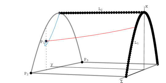
Figure 1: The state space of the loaf of bread system for the stiff equation of state $\rho=p+\rho_{\rm s}$. The equilibrium points, indicated as bold dots in the figure, are denoted as in table 1. The figure also displays the combined limiting orbit described in section 3, corresponding to the limit of infinite central pressure within the family of regular center orbits. The RSI part of this combined orbit, which completely lies in the boundary $Y=1$, starts out from the $Y=1$ point on $L_{2}$ and spirals into $P_{1}$. However, from the figure it is not at all clear that the RSI orbit actually spirals into $P_{1}$, which is explained by the fact that the absolute value of the quotient $q$ between the imaginary and the negative real part of the relevant complex conjugate eigenvalues is not very large, the precise value being $q=\sqrt{3}$. This implies that the distance to $P_{1}$ decreases by a factor $e^{-2\pi/q}\approx 0.026$ for every turn around $P_{1}$. The skeleton part of the combined orbit, around which the surface of regular orbits is rolled, is for this particular equation of state confined to the plane $\Sigma=1/2$.

6 Some multiple neck optical geometries

Here we investigate the interior solution for different equations of state. Our present purpose is to show that the interior optical geometry will look quite different for the different cases. We showed in an earlier paper [5] that the geometry may develop additional “necks” and “bulges” corresponding to unstable and stable closed lightlike orbits respectively. As shown by Chandrasekhar and Ferrari [14] the axial modes of nonradial metric perturbations of SSS perfect fluids are (to first order) not coupled to a perturbation of the matter. Such metric perturbations may therefore be interpreted as pure gravitational waves. By separation of variables the equations governing these modes can be reduced to the 1-dimensional Schrödinger equation

$$-\frac{d^{2}}{dr_{\!*}^{2}}Z_{l}+VZ_{l}=\sigma^{2}Z_{l}$$ (39)

where the total potential $V=V_{l}+V_{m}$ is dominated by $V_{l}=l(l+1)\tilde{r}^{-2}$, $l=2,3,\ldots$ which is simply the effective potential for photons with angular momentum $L^{2}=l(l+1)$. This, together with the fact that the correction $V_{m}$ to the total potential is small compared to $V_{l}$ in most cases, shows that the optical geometry is closely related to the trapped modes of gravitational radiation since the maxima and minima of $V_{l}$ clearly correspond to the necks and bulges of the optical geometry respectively.

We turn, now, to the analysis of the optical geometry of some different models. In the case of a double layer uniform density model the equation of state is parametrized by the constant densities $\rho_{+}$ and $\rho_{-}$ of the interior and exterior zones respectively, as well as the transition pressure $p_{\mathrm{t}}$ where the density is discontinuous. In the single layer uniform density model considered by Abramowicz et. al. [2] the only parameter is the density $\rho_{0}$, and the linear model is parametrized by the central and surface density $\rho_{\rm c}$ and $\rho_{\rm s}$ respectively. Given these parameters, each stellar model is obtained by specifying the central pressure $p_{\mathrm{c}}$.

Below we display and compare the optical geometry for these models. The parameter values for the two-zone models are chosen to obtain three distinct examples of optical geometries with pronounced double necks, corresponding to two deep potential wells as shown in [5]. They were chosen to have the same value of the tenuity $\alpha:=R/M=2.2749$, as well as the same mass. This condition is visualized by letting the exterior geometry be identical in each triplet of figures. The chosen parameters are shown in table 3, where we have chosen to use cgs-units and assigned a mass of $1.5M_{\odot}$ to each model. We see that the central density required to produce the double neck structure is very large. We could have chosen to have a more realistic central density, but then the total mass of the corresponding stellar object would have been of the order of several hundred solar masses.

In figure 2 we compare a two-zone model with a uniform density model, and a model with a linear equation of state. The parameters of the two-zone model were chosen so that the bulges should have approximately the same size corresponding to two equally shaped potential wells. The density of the uniform model were then chosen to give the same tenuity as this model. The parameters of the linear model were chosen so that the single neck should be reasonably visible. The tenuity of this model is $\alpha=2.81$ which is close to the limit $\alpha_{\mathrm{m}in}=2.749$ for this type of equations of state. The lower part of the double layer model is of course, as in the uniform case, a sphere. We thus expect that the modes of the inner potential well, granted that the inner neck is thin, should resemble those of the uniform model.

In figure 3 we look at three different two-zone models. The first is the one already shown in figure 2. The two other models are chosen to display the possibility to have either a large upper bulge or a large lower one.

It would be interesting to know if the two-zone models are stable against small radial perturbations, but this question turns out to be nontrivial. Of course, a star with constant density is always stable, however since this configuration is very unphysical (the speed of sound diverges) one usually views the equation of state $\rho$ = constant as an approximation to the more physical $\rho=\rho_{0}+\rho_{1}(p)$, where $\rho_{0}$ is a constant and $\rho_{1}(p)$ is a function of the pressure satisfying $\rho_{1}(p)\ll\rho_{0}$ for all $p<p_{\rm c}$. One may then impose reasonable conditions on this equation of state, for instance causality ($v_{\rm{sound}}\leq 1$), and the dominant energy condition ($\rho\leq p$). It seems however that you cannot find any reasonable functions $\rho_{1}(p)$ such that these conditions hold and the star is ultrarelativistic. We may note that none of our two-zone models respects the dominant energy condition. Ignoring these physical difficulties and viewing the models as toys, we may proceed with the stability analysis. Firstly we may remark that you cannot use the usual analysis of the mass to radius curve to establish stability properties for any model with constant density since the adiabatic index is not defined [15] (it is determined by the small function $\rho_{1}(p)$ which is arbitrary here). We are therefore forced to try a dynamical approach, but here the analysis is complicated by the discontinuity in the perturbation equation so that the differential equation is no longer of the standard Sturm-Liouville type. Therefore, the standard theorems of Sturm-Liouville theory cannot be directly applied. However, since the discontinuous density function can be arbitrarily well approximated by a continuous function one might expect that nothing too extraordinary happens. Preliminary results using a variational principle indicate that this is indeed the case. The stability of more realistic ultracompact (in the sense $R\leq 3M$) stellar configurations with a phase transition has previously been studied by Iyer, Vishvehvara and Dhurandhar [16]. They conclude that there exist stable causal ultracompact models, however not with any of the high density equations of state proposed in the litterature at that time.

Two-zone models	$\rho_{+}(g/cm^{3})$	$\rho_{-}(g/cm^{3})$	$p_{\rm t}(g/cms^{2})$	$p_{\rm c}(g/cms^{2})$	$r_{\rm t}/R$
Peanut	$2.74\times 10^{19}$	$5.48\times 10^{15}$	$3.52\times 10^{38}$	$5.67\times 10^{41}$	0.014
Bigup	$5.81\times 10^{19}$	$5.51\times 10^{15}$	$2.90\times 10^{38}$	$5.22\times 10^{41}$	0.010
Bigdown	$2.80\times 10^{19}$	$5.48\times 10^{15}$	$3.63\times 10^{38}$	$2.90\times 10^{42}$	0.014

Other models	$\rho_{\rm c}(g/cm^{3})$	$\rho_{\rm s}(g/cm^{3})$	$p_{\rm c}(g/cms^{2})$
Uniform density	$5.56\times 10^{15}$		$7.59\times 10^{37}$
Linear	$9.00\times 10^{16}$	$5.56\times 10^{15}$	$7.59\times 10^{37}$

Table 3: Parameter values for the models considered. Here we have chosen the mass of the object to be $1.5M_{\odot}$ which means that the radius will be about $6.2$ km for the linear model, and $5.0$ km for the others. We see that the term ultracompact is indeed relevant since these objects are denser than normal neutron stars are believed to be. We see that the two-zone models consist of very dense, small cores ($r_{\rm t}$ refers to the radius where the phase transition takes place), and envelopes of more realistic densities.

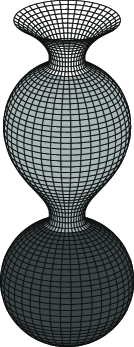
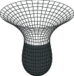
Figure 2: The optical geometry of the “peanut” model compared with the uniform and the linear models. All models have the same mass and hence identical exterior geometry.

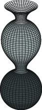
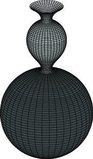
Figure 3: The optical geometry of the “peanut” model compared with the “bigup” and “bigdown” models. All models have the same mass and hence identical exterior geometry.

7 Concluding remarks

The two-zone models discussed in this paper could be considered as toy models for stars having a first order phase transition in their interiors. Our results indicate that a phase transition is an important mechanism for producing a pronounced neck in the optical geometry of a stellar model. In this picture, the outer neck at $r=3M$ (if it exists) is associated with the vacuum/matter phase transition at the surface of the star. However, this is not the only mechanism for producing necks. Another example is provided by the stiff linear equation of state. In that case there is an increasingly long sequence of shallow necks which is associated with the high density spiral equilibrium point $P_{1}$[4].

The existence of multiple neck optical geometries is associated with gravitational perturbation potentials with multiple wells [5]. It would therefore be of interest to calculate the corresponding quasi-normal modes along the lines of calculations done for single well potentials in [1] (uniform density models) and in [17] (polytropic models).

References

- [1] S. Chandrasekhar and V. Ferrari, Proc. Roy. Soc. Lond. A 434, 449 (1991).
- [2] M. A. Abramowicz et al., Class. Quantum Grav. 14, L189 (1997).
- [3] K. Rosquist, Phys. Rev. D 59, 044022 (1999), (gr-qc/9809033).
- [4] M. Karlovini, K. Rosquist, and L. Samuelsson, Ultracompact stars with multiple necks, 2000, gr-qc/009073.
- [5] M. Karlovini, K. Rosquist, and L. Samuelsson, Annalen der Physik 9, 149 (2000).
- [6] U. S. Nilsson and C. Uggla, General relativistic static stars: Linear Equations of State, 2000, gr-qc/0002021.
- [7] U. S. Nilsson and C. Uggla, General relativistic static stars: Polytropic Equations of State, 2000, gr-qc/0002022.
- [8] L. Lindblom, Phys. Rev. D 58, 024008 (1998).
- [9] L. Lindblom and A. K. M. Masood-ul-Alam, in Directions in General Relativity II: Papers in Honor of Dieter Brill, edited by B. L. Hu and T. A. Jacobson (Cambridge University Press, Cambridge, 1993), p. 172.
- [10] C. W. Misner and D. H. Sharp, Phys. Rev. 136, 571 (1964).
- [11] B. K. Harrison, K. S. Thorne, M. Wakano, and J. A. Wheeler, Gravitation theory and gravitational collapse (University of Chicago Press, Chicago, USA, 1965).
- [12] C. W. Misner, K. S. Thorne, and J. A. Wheeler, Gravitation (Freeman, San Fransisco, USA, 1973).
- [13] R. C. Tolman, Phys. Rev. 55, 364 (1939).
- [14] S. Chandrasekhar and V. Ferrari, Proc. Roy. Soc. Lond. A 432, 247 (1991).
- [15] K. S. Thorne, in Proccedings of the international school of physics “Enrico Fermi”, edited by L. Gratton (Academic Press, New York and London, 1966), p. 166.
- [16] B. R. Iyer, C. V. Vishveshwara, and S. V. Dhurandar, Class. Quantum Grav. 2, 219 (1985).
- [17] N. Andersson and K. D. Kokkotas, Mon. Not. R. Ast. Soc. 297, 493 (1998).