A data-analysis strategy for detecting gravitational-wave signals from inspiraling compact binaries with a network of laser-interferometric detectors

Abstract

A data-analysis strategy based on the maximum-likelihood method (MLM) is presented for the detection of gravitational waves from inspiraling compact binaries with a network of laser-interferometric detectors having arbitrary orientations and arbitrary locations around the globe. For simplicity, we restrict ourselves to the Newtonian inspiral waveform. However, the formalism we develop here is also applicable to a waveform with post-Newtonian (PN) corrections. The Newtonian waveform depends on eight parameters: the distance $r$ to the binary, the phase $\delta_{c}$ of the waveform at the time of final coalescence, the polarization-ellipse angle $\psi$, the angle of inclination $\epsilon$ of the binary orbit to the line of sight, the source-direction angles $\{\theta,\phi\}$, the time of final coalescence $t_{c}$ at the fiducial detector, and the chirp time $\xi$. All these parameters are relevant for a chirp search with multiple detectors, unlike the case of a single detector. The primary construct on which the MLM is based is the network likelihood ratio (LR). We obtain this ratio here. For the Newtonian inspiral waveform, the LR is a function of the eight signal-parameters. In the MLM-based detection strategy, the LR must be maximized over all of these parameters. Here, we show that it is possible to maximize it analytically with respect to four of the eight parameters, namely, $\{r,\delta_{c},\psi,\epsilon\}$. Maximization over the time of arrival is handled most efficiently by using the Fast-Fourier-Transform algorithm, as in the case of a single detector. This not only allows us to scan the parameter space continuously over these five parameters but also cuts down substantially on the computational costs. The analytical maximization over the four parameters yields the optimal statistic on which the decision must be based. The value of the statistic also depends on the nature of the noises in the detectors. Here, we model these noises to be mainly Gaussian, stationary, and uncorrelated for every pair of detectors. Instances of non-Gaussianity, as are present in detector outputs, can be accommodated in our formalism by implementing vetoing techniques similar to those applied for single detectors. Our formalism not only allows us to express the likelihood ratio for the network in a very simple and compact form, but also is at the basis of giving an elegant geometric interpretation to the detection problem. Maximization of the LR over the remaining three parameters is handled as follows. Owing to the arbitrary locations of the detectors in a network, the time of arrival of a signal at any detector will, in general, be different from those at the others and, consequently, will result in signal time-delays. For a given network, these time delays are determined by the source-direction angles $\{\theta,\phi\}$. Therefore, to maximize the LR over the parameters $\{\theta,\phi\}$ one needs to scan over the possible time-delays allowed by a network. We opt for obtaining a bank of templates for the chirp time and the time-delays. This means that we construct a bank of templates over $\xi$, $\theta$, and $\phi$. We first discuss “idealized” networks with all the detectors having a common noise curve for simplicity. Such an exercise nevertheless yields useful estimates about computational costs, and also tests the formalism developed here. We then consider realistic cases of networks comprising of the LIGO and VIRGO detectors: These include two-detector networks, which pair up the two LIGOs or VIRGO with one of the LIGOs, and the three-detector network that includes VIRGO and both the LIGOs. For these networks we present the computational speed requirements, network sensitivities, and source-direction resolutions.

I Introduction

The existence of gravitational waves, which is predicted in the theory of general relativity, has long been verified ‘indirectly’ through the observations of Hulse and Taylor [1]. The inspiral of the members of the binary pulsar system named after them has been successfully accounted for in terms of the back-reaction due to the radiated gravitational waves [1, 2]. However, detecting such waves with man-made ‘antennas’ has not been possible so far. Nevertheless, this problem has received a lot of attention this decade, especially, due to the arrival of laser-interferometric detectors, which are expected to have sensitivities close to that required for detecting such waves.

A gravitational-wave (GW) source that is one of the most promising candidates for detection by Earth-based interferometric GW detectors is the inspiraling compact binary [3]. Present estimates show a significant number of coalescence events every year of such binaries that produce waves strong enough to be detectable by current detectors during their inspiral phase, a few seconds before the onset of coalescence. Moreover, the time-evolution of these waveforms (chirps) is well understood in the frequency band where the present interferometric detectors are most sensitive.

In the past, a sizable amount of research has been done on the problem of detecting gravitational waves using a single bar or interferometric detector. However, very little work has been devoted to develop techniques to analyze the data from a network of such detectors. Searching for chirps using a network of detectors is gaining importance due to (a) its superior sensitivity vis à vis that of a constituent detector and (b) improving feasibility for a real-time computational search. As has been argued before (see, e.g., Ref [4]), for a given false-alarm probability, the threshold for detection is lowered as the number of detectors is increased. This increases the probability of detection by ‘coherently’ analyzing the signals from a network rather than a single detector. One can think of simpler approaches to the network problem where one matches event lists from different detectors in the network and sets up thresholds on the estimated parameter differences. Indeed, in the past, a formalism for interpreting coincidences of burst events in a pair of detectors has been suggested by Schutz and Tinto [5]. However, such approaches, even if they were extended to the case of chirps, would be non-optimal, because they do not use the phase information of a signal at different detectors. The coherent search strategy described here crucially uses phase information.

One of the early papers that came close to discussing the problem of detecting a Newtonian chirp using a network optimally was that of Finn and Chernoff [6]. This paper observed that since the orientations of the two LIGO detectors were very similar, their joint sensitivity was larger than any one of them. Bhawal and Dhurandhar also addressed the issue of detection using multiple detectors [7]. Their main aim was to find the optimal recycling mode of operation of the planned laser interferometric detectors for which a meaningful coincidence detection of broadband signals could be performed. However, the issue of how a network of detectors with arbitrary orientations and arbitrary locations on the globe can be optimally used as a “single” detector of sensitivity higher than that of any of its subsets of individual detectors was not addressed in these earlier papers.

Use of a detector network has nevertheless received considerable attention in the context of the parameter estimation problem. A formalism for using the responses of multiple detectors, in the absence of noise, to infer the parameters of a chirp (also known as the “inverse problem”) was developed by Dhurandhar and Tinto [8, 9]. Some of the other notable works that address this issue in the presence of noise are Refs. [10, 11, 12]. The prime motivation behind using a network in this regard is that the larger the number of detectors, the smaller are the errors in estimated values of the binary parameters. However, the starting point in these approaches is the assumption that the problem of detection has already been addressed and the detector-specific chirp-templates that result in “super-threshold” cross-correlations with the individual detector outputs, have been picked.

A formalism was developed in Ref. [13] that sought an optimal detection strategy for chirps in the simplifying case of a network with closely located laser-interferometric detectors and with idealized detector noise. This work was based on a coherent search. Its main result was that the optimal statistic for a network of up to three such detectors was proven to be the sum of the signal-to-noise (SNR) ratios of the individual detectors. It was also shown that the sensitivity of such a network improved as roughly the square-root of the number of detectors in the network. This formalism was extended to the case of arbitrarily located detectors in Ref. [14], which showed a way to reduce the network statistic such that the number of chirp parameters over which a numerical search is required for detecting chirps drops from eight to three. This paves the way for a vast reduction in computational speed requirements and makes a multiple detector search for chirps much more feasible. One of the main aims of this paper is to formulate a data-analysis strategy that implements these formal findings in the case of existing and upcoming networks and to provide estimates on the required computational speeds, etc.

As the members of a binary orbit around their center of mass, they lose energy in the form of gravitational waves. This results in their inspiral. Consequently, they emit gravitational waves with monotonically increasing amplitude and frequency [15]. Although the gravitational waveform originating from an inspiraling binary is known accurately up to the 2.5 post-Newtonian (PN) order [16], nevertheless as a first calculation we limit our study to the detection of the Newtonian chirp. This is because our primary aim here is to develop the new formalism, namely, that of optimally using the data from a network of detectors to detect a chirp. We find evidence of the applicability of our formalism to higher post-Newtonian orders. We also find for the Newtonian signal that there is essentially no correlation between the parameters describing the masses and the direction angles to the source when the noise curves are assumed to be identical for all the detectors in the network. This has the following important implications: The total number of templates is then just a product of number of templates for a single detector and the number of templates needed to scan source directions. If this property holds also for the PN case, then, in effect, we need to obtain the number of templates for the directions only and club together with this the information we have on the number of templates for a PN signal in a single detector. We hope to address this issue in detail in future work.

In our analysis, we assume that the noise in each detector is predominantly stationary and Gaussian, with occasional contamination from non-Gaussian events. Indeed, the real data stream from the detectors is not expected to be purely stationary and Gaussian, unlike what is assumed in most of the GW data-analysis literature thus far. In fact, the data from the Caltech 40 meter prototype interferometer have the expected broadband noise spectrum, but superposed on this are several other noisy features [17], such as long-term sinusoidal disturbances arising from suspensions and electric-main harmonics, which have been studied in other works [18, 19]. There are also transients occurring every few minutes, typically due to servo-controls instabilities or mechanical relaxation in suspension systems, etc. Adaptive methods are being explored to combat high amplitude ring-downs and sinusoids occurring in the data [20], by effectively removing them from the data, so that the data are ‘cleaned’ from these non-Gaussian features. In the improved detectors of the future, it is expected that the noise will tend to Gaussianity, and may only be occasionally contaminated by non-Gaussian events. It is in this spirit that our above assumption about the noise must be taken. The strategy we adopt in dealing with such a detector noise is to assume it to be stationary and Gaussian for the purposes of our statistical analyses. Such an assumption is justified in practice provided one vetoes out detections due to the occasional non-Gaussian events occurring in the data obtained from the detectors. The vetoing criterion we propose is an extension of the $\chi^{2}$ criterion used in Ref. [17]. This model of the noise is simple enough so that analytical methods can be used for the approach we take.

We also assume that noises to be uncorrelated among different pairs of detectors. When the detectors are widely separated around the globe, correlations among the noises of different detectors are expected to be negligible, and our assumption remains valid for such a case. For most networks of proposed detectors this is true, unless it consists of the two coincident detectors at Hanford. In that case, a more general analysis is necessary that takes into account possible correlations between the noises in different detectors. Such an approach is being pursued by Finn [21]. The only other assumption we make on the detector noise is that it is additive.

We use the maximum-likelihood method for optimizing the detection problem. The problem is formulated by obtaining a single likelihood-ratio (LR) for the entire network. We define the “network output”, ${\sf x}$, as a single network-vector, the components of which are the individual detector outputs. Similarly, the “network signal”, ${\sf s}$, is defined to be a single network-vector, the components of which are the individual detector signals. Since we assume the noise in different detectors to be independent, the probability density function (PDF) for the noise of the network is just a product of the PDFs of noise in the individual detectors. The LR is then a simple expression in terms of the norm of ${\sf s}$ and the inner product of ${\sf x}$ and ${\sf s}$. In this form, the LR is a function of a complete set of eight independent parameters that characterize the Newtonian chirp signal of an inspiraling binary.

For the assumptions made on the detector noises, a network’s logarithmic likelihood ratio (LLR) turns out to be the sum of the individual detector’s LLRs. The form of LLR allows us to deduce the network matched-filter in a straightforward way; it turns out to be an $M$-dimensional vector with components that are just the normalized single detector templates of Sathyaprakash and Dhurandhar [22] (henceforth referred to as SD). Inferring this network-template is the second result of this paper. The problem of detection then reduces to the maximization of LLR over the parameters and comparing its maximized value with the pre-determined detection threshold. We argue that this step can be implemented in a way similar to the one suggested in SD.

To obtain the maximum likelihood ratio (MLR), the LR has to be maximized over the eight parameters: the distance to the binary system $r$, the phase of the waveform at the time of coalescence $\delta_{c}$, the polarization-ellipse angle $\psi$, the inclination of the binary orbit $\epsilon$, the direction angles $\{\theta,\phi\}$, the time of final coalescence at the fiducial detector $t_{c}$, and the chirp time $\xi$. In principle, this can always be done numerically using a grid in the eight dimensional parameter space. In practice, such a strategy is not only computationally infeasible but, as we show in this paper, is also wasteful. The first important result in this paper is a new representation for the signal, which is expressed here in terms of the complex expansion coefficients of the wave and the detector tensor in a basis of symmetric, trace-free (STF) tensors of rank $2$. Such a representation of the signal not only allows us to express the LR for the network in a very simple and compact form, but also brings out the symmetries in the response functions of the detectors and is at the basis of giving a novel geometric interpretation to the detection problem. Maximization of the LR over four of the eight parameters can be performed analytically using the symmetries in the responses, which are clearly brought out when the responses are expressed in terms of the Gel’fand functions. Further, the Fast Fourier transform (FFT) can be used to maximize the LLR over the parameter $t_{c}$, as in the case of a single detector. The network template is constructed by taking into account appropriate time-delays at the individual detector sites.

The analytic maximization and the FFT have the following advantages:

1. They allow us to scan continuously the parameter space for the five parameters $r,\delta_{c},\epsilon,\psi$ and $t_{c}$.

2. They save substantially on the computational cost.

We are then left with the three parameters, namely, $\xi$, $\theta$, and $\phi$. A full sky search over $(\theta,\phi)$ maps to a time-delay window, consisting of all possible time-delays, for a given network. The search over the time-delay window may be performed by using the samples of the cross correlations between the signal and the detector outputs or by constructing a template bank. The latter approach has the advantage of incorporating the desired mismatch related to the fractional loss in signal-to-noise ratio. Turning the argument around, the template bank can also be used as guideline to re-sample the data at a rate that is consistent with the desired mismatch and then scan over all samples in the time-delay windows. We, therefore, opt to construct a template bank in $\xi$, $\theta$, and $\phi$. This is efficiently obtained by first computing the metric as given by Owen [23]. We then obtain the volume of the parameter space, given the metric, and divide this volume by the volume spanned by a template to obtain the number of templates. From this information, we can easily evaluate the computational costs for the search. Secondly, the metric is essentially the Fisher information matrix and its inverse yields the covariance matrix from which errors in the parameters can be obtained.

We apply our formalism to analyze several networks of detectors. First, we examine idealized networks, with all detectors having the LIGO-I noise. Such an exercise nevertheless yields useful estimates of computational costs while at the same time simplifying the calculations and providing invaluable insights. We then consider the LIGO-VIRGO network with their respective noise curves. The computations for this case are done numerically. For these networks we estimate the computational speed requirements, sensitivities, and the resolution in the direction to the source. We find that the computational costs are high even for the two-detector network. The online data processing speeds required are in terms of Gflops and for a 3 detector network the online speeds needed escalate to few tens of Tflops. The costs would go up further when PN corrections are incorporated into the waveform. For example, for LIGO-I noise and allowing a maximum mismatch of $3\%$ between the signal and the template, the number of templates required increases by a factor of about 4 or 5 [24]. Hence, even for a network searching for PN-corrected waveforms, one may expect the computational costs to increase by similar factor. Clearly, our results show that use of hierarchical search methods are called for. Assuming the individual masses to be greater than $0.5M_{\odot}$, and with LIGO-I noises in the detectors at Hanford and Louisiana, the online computing speed requirement is $12$ Gflops, for a $3\%$ mismatch between the signal and the template. The corresponding figure for one of the LIGO detectors and VIRGO is $170$ Gflops. For the three detector LIGO-VIRGO network, the cost rises to few tens of Tflops. The sensitivity roughly scales as $\sqrt{M}$ or a little less, where $M$ is the number of detectors. The resolution in direction is about a fraction of a degree for the networks where we have assumed LIGO-I noise and a signal-to-noise ratio of 12.

The paper is organized as follows. We begin by setting up in Sec. II the basic mathematical framework required for our formalism. This includes a discussion of the various relevant coordinate frames and their relationships with one other. We also introduce the wave and detector tensors, using which we define the signal at a detector. The signal at a detector is then used to define the network signal and infer the network statistic. In Sec. III, we present the Newtonian chirp in its familiar form. This allows us to define the role of each parameter influencing the waveform. It also introduces important notations that we follow in the rest of the paper. We then derive a less familiar expression for the signal induced by a chirp in a detector. This new representation for the chirp-signal simplifies the analysis associated with a network-based detection strategy. In Sec. IV, we show how the detection problem can be optimally addressed using the maximum-likelihood method. We present a single likelihood ratio for the entire network. It has a very simple form owing to our use of the new representation for the signal. The LR is analytically maximized first with respect to $r$ and $\delta_{c}$ in the well established way [22, 13], and then with respect to $\psi$ and $\epsilon$ using the symmetry properties of the detector responses [14]. We then show how the FFT can be used to efficiently maximize over the time of final coalescence or, alternatively, the time of arrival at a fiducial detector. This is followed by a construction of the network template and the network correlation-vector. The window consisting of all possible time-delays is discussed. In Sec. V, we construct the template bank on the rest of the parameter space, i.e., on $\{\xi,\theta,\phi\}$ by extending Owen’s [23] method and present a way of arriving at the number of templates required. We then give expressions for the computational costs and the resolutions achievable in parameter values. Sec. VI is devoted to the discussion of several networks including the realistic network of LIGOs and VIRGO. In Sec. VII, we discuss the statistical properties of the optimal network statistic. We calculate the false-alarm and the detection probabilities associated with the network statistic, and obtain a relation between the network sensitivity and the number of detectors in a network. We also discuss the case where the detector noise is contaminated by non-Gaussian noise events and suggest a vetoing criterion based on the $\chi^{2}$ - test.

We use the following convention for symbols in this paper, unless otherwise specified. When it is useful to keep track of the complex nature of a network-based or individual detector-based variable we denote it by an uppercase Roman letter, whereas the lower case letters are reserved for real variables. Network-based vectors are displayed in the Sans Serif font. The label $I$ in the superscript or subscript of a variable denotes a (real) natural number that associates it with a particular detector. It ranges from $1$ to $M$, where $M$ is the total number of detectors in a network. It can be considered as a vector index over detectors. We use the index I for several of the network variables. However, certain quantities that do not obviously display a vector character, but still pertain to a detector, $I$, are denoted by enclosing the index in parentheses. Einstein summation convention over repeated indices is used for brevity, unless explicitly stated.

II Mathematical framework

A Reference Frames

Our first aim is to obtain a quantity that would define the response of an arbitrary network of broadband detectors to an incoming gravitational wave. In this quest, it is important to understand how the responses of arbitrarily oriented and arbitrarily located individual detectors to such a wave relate to one another. This is aided by introducing the three different frames of reference that arise naturally in such a problem, namely, $(i)$ the wave frame, $(ii)$ the network frame, and $(iii)$ the frame of a representative detector in the network. We define these reference frames in terms of the following right-handed, orthogonal, three-dimensional Cartesian coordinates:

$(i)$ Wave frame: We associate with this frame the coordinates $(X,Y,Z)$. The gravitational wave, which is assumed to be weak and planar, is taken to travel along the positive $Z$-direction; then $X$ and $Y$ denote the axes of the polarization ellipse of the wave.

$(ii)$ Network frame: There is no unique definition of this frame. For Earth-based detectors being discussed here, if the network has a large number of detectors (say, $M>3$), a convenient choice is a frame attached to the center of the Earth. Let the coordinate system that defines this frame be $(x_{E},y_{E},z_{E})$. The $x_{E}$ axis lies along the line joining Earth’s center and the equatorial point that lies on the meridian passing through Greenwich, England. It points radially outwards. The $z_{E}$ axis is chosen to lie in the direction of the line passing through the center of Earth and the north pole. The $y_{E}$ axis is chosen to form a right-handed coordinate system with the $x_{E}$ and $z_{E}$ axes.

For a network consisting of $M\leq 3$ detectors, certain calculations can be simplified by using the fact that the corner stations (or hubs) of all the detectors will lie on a single plane. Specifically, for $M=3$ we define the network frame such that one of the detectors is at its origin, a second detector is on one of the coordinate axes, say, $z$, and the third lies on one of the coordinate planes containing the $z$ axis, say, the $x-z$ plane. Later in the text when we consider various examples of three-detector networks, we choose this as the network frame.

$(iii)$ Detector frame: Let $(x_{(I)},y_{(I)},z_{(I)})$ (with $I$ = 1,2,…,M) denote the orthogonal coordinate frame attached to the detector labeled $I$. The $(x_{(I)},y_{(I)})$ plane contains the detector arms and is assumed to be tangent to the surface of the Earth. The $x_{(I)}$ axis bisects the angle between the detector’s arms. The direction of the $y_{(I)}$ axis is chosen in such a way that $(x_{(I)},y_{(I)},z_{(I)})$ form a right-handed coordinate system with the $z_{(I)}$ axis pointing radially out of Earth’s surface.

Apart from the above choices for frames, we define a fourth frame, namely, the frame of a “fiducial” detector (henceforth referred to as the “fide”). This frame serves as a reference frame with respect to which the locations or orientations of each of the detectors in a network shall be specified. Indeed, we will develop our whole formalism for a general network using the fide frame as a reference. It is only towards the end, when we consider specific cases of networks, shall we identify the fide frame with one of the three frames defined above, depending upon suitability.

Physical quantities in these frames are related by orthogonal transformations that rotate one frame into another. These orthogonal transformations are defined in terms of three sets of Euler angles that specify the orientation of one frame with respect to another. To understand these relations, let ${\cal O}$ be an orthogonal transformation matrix. Let $(\phi,\theta,\psi)$ be the Euler angles through which one must rotate the fide frame to the align with the wave frame. Then

$${\sf x}_{\rm wave}={\cal O}(\phi,\theta,\psi){\sf x}_{\rm fide}\ \ ,$$ (1)

where ${\sf x}_{\rm fide}$ denote the axes of the fide frame and ${\sf x}_{\rm wave}$, those of the wave frame. The transformation is an orthogonal matrix given by [25]

$${{\cal O}(\phi,\theta,\psi)=\left(\begin{array}[]{ccc}\cos\psi\cos\phi-\cos\theta\sin\phi\sin\psi&\cos\psi\sin\phi+\cos\theta\cos\phi\sin\psi&\sin\psi\sin\theta\\ -\sin\psi\cos\phi-\cos\theta\sin\phi\cos\psi&-\sin\psi\sin\phi+\cos\theta\cos\phi\cos\psi&\cos\psi\sin\theta\\ \sin\theta\sin\phi&-\sin\theta\cos\phi&\cos\theta\end{array}\right)\,.}$$ (2)

Similarly, if $(\alpha_{(I)},\beta_{(I)},\gamma_{(I)})$ are the Euler angles that rotate the fide frame to the frame of the $I$-th detector, then

$${\sf x}_{\rm detector_{(I)}}={\cal O}(\alpha_{(I)},\beta_{(I)},\gamma_{(I)}){\sf x}_{\rm fide}\ \ ,$$ (3)

where ${\sf x}_{\rm detector_{(I)}}$ denote the axes of the $I$-th detector frame.

One can imagine yet another frame attached to the source whose $z$ axis is along the orbital angular-momentum vector of the binary. The angle, $\epsilon$, between this vector and our line of sight to the binary is termed as the inclination angle and has the range $[0,\pi]$. The associated $x-y$ plane specifies the plane of the binary. It is then possible to orient the $x$ and $y$ axes on this plane in such a way that a rotation of the wave frame through the Euler angles, $(0,\epsilon,0)$, aligns it with the source frame.

B Wave tensor, detector tensor, and beam-pattern functions

A gravitational wave can be represented by metric tensor fluctuation, $h_{\mu\nu}$, about the background space-time which we take to be flat. The subscripts $\mu$ and $\nu$ denote space-time indices. In the transverse trace-free (TT) gauge, the non-vanishing components of $h_{\mu\nu}$ in the wave frame are $h_{xx}=-h_{yy}\>{\equiv}\>h_{+}$, $h_{xy}=h_{yx}\>{\equiv}\>h_{\times}$. Here, $h_{+}$ and $h_{\times}$ are the two linear-polarization components of the wave. When a metric fluctuation specifically represents a gravitational wave, its spatial part is identified as twice the wave tensor, $w_{ij}$, where $i$ and $j$ refer to space indices and take values $1,2$, and $3$ (see Ref. [8]). In the TT gauge, the wave tensor is a symmetric trace-free (STF) tensor of rank 2. In any arbitrary frame, the wave tensor can be expressed in terms of its circular-polarization components as,

$$w^{ij}(t)={1\over 2}\left[(h_{+}(t)+ih_{\times}(t))e_{R}^{ij}+(h_{+}(t)-ih_{\times}(t))e_{L}^{ij}\right]\ \ ,$$ (4)

where $e_{R,L}^{ij}$ are the right and left-circular polarization tensors, respectively. The $e_{R,L}^{ij}$ are both second rank STF tensors and obey the orthonormality conditions,

$$e_{L,\>R}^{ij}\>e_{L,\>R\>ij}^{*}=1\>,\quad e_{L,\>R}^{ij}\>e_{R,\>L\>ij}^{*}=0\ \ ,$$ (5)

where a star denotes complex conjugation. The reality of the wave tensor ensures that

$$e_{L}^{ij\>*}=e_{R}^{ij}\,.$$ (6)

Using (6), the wave-tensor expression (4) simplifies to

$$w^{ij}(t)=\Re\left[\left(h_{+}(t)+ih_{\times}(t)\right)e_{R}^{ij}\right]\ \ ,$$ (7)

where $\Re[A]$ denotes the real part of a complex quantity $A$.

In an arbitrary reference frame, the polarization tensor can be expressed as

$$e_{L}^{ij}=m^{i}m^{j}\ \ ,$$ (8)

where the $m^{k}$ is the $k$-th component of a complex null vector $\sf m$ in that reference frame. It is defined as

$$m^{k}=\frac{1}{\sqrt{2}}(e_{X}^{k}+ie_{Y}^{k})\ \ ,$$ (9)

where ${\bf e}_{X}$ and ${\bf e}_{Y}$ are unit vectors in the $X$ and $Y$ direction of the wave axes, respectively [8]. The above expression shows that the $e_{R,L}^{ij}$ are STF tensors of rank 2. Hence, they can be expanded in a basis of STF-2 tensors, ${\cal Y}^{ij}_{2n}$, (see appendix A):

$$e_{R}^{ij}=\sqrt{8\pi\over 15}T_{-2}{}^{n}{\cal Y}^{ij}_{2n}\quad{\rm and}\quad e_{L}^{ij}=\sqrt{8\pi\over 15}T_{2}{}^{n}{\cal Y}^{ij}_{2n}\ \ ,$$ (10)

where the expansion coefficients, $T_{\pm 2}{}^{n}$, with $n=0,\pm 1,\pm 2$, are Gel’fand functions [26]. (For a more elaborate discussion on these functions see Refs. [8, 9].) These functions depend on the Euler angles through which one must rotate the reference frame to the wave frame. If the reference frame is chosen to be the fide, then these angles are just $(\phi,\theta,\psi)$. While implementing more than a single frame-transformation in relating these two frames, the addition theorem (A4) for Gel’fand functions is used to obtain the required wave tensor. In such a case, the wave tensor depends on more than one set of Euler angles.

The $I$-th detector tensor, $d_{ij}^{I}$, is given by

$$d_{ij}^{I}=n_{(I)1i}n_{(I)1j}-n_{(I)2i}n_{(I)2j}\ \ ,$$ (11)

where ${\sf n}_{(I)1}$ and ${\sf n}_{(I)2}$ are the unit vectors along the arms of the $I$-th interferometer, which is taken to have orthogonal arms. Like the polarization tensors, even $d_{ij}^{I}$ is an STF tensor of rank 2. Hence, in any frame it can be expanded in a basis of STF-2 tensors. In such a basis, the components of $d_{ij}^{I}$ can be expressed in terms of Gel’fand functions, $T_{\pm 2}{}^{n}$ (see Eq. (B3)). In the fide frame, these functions depend on the Euler angles $\{\alpha_{(I)},\beta_{(I)},\gamma_{(I)}\}$, which specify the relative orientation of the $I$-th detector with respect to the fide.

When detectors are distributed around the globe there are, in general, relative delays in the arrival times of a particular phase of a given wave at different locations. Let $\tau_{(I)}(\theta,\phi)$ be the relative delay between the arrival times at the $I$-th detector and the fide, where the source direction is given by $(\theta,\phi)$. If ${\hat{\sf n}}(\theta,\phi)$ is the unit vector along the direction of the wave, i.e., ${\hat{\sf n}}(\theta,\phi)={\hat{\sf Z}}$, then

$$\tau_{(I)}(\theta,\phi)={{({\sf r}_{(I)}-{\sf r}_{(f)})\cdot{\hat{\sf n}(\theta,\phi)}}\over{c}}\ \ ,$$ (12)

where ${\sf r}_{(I)}$ and ${\sf r}_{(f)}$ are the position vectors of the $I$-th detector and fide, respectively, with respect to any given reference frame. Note that $\tau_{(I)}(\theta,\phi)$ can take positive as well as negative values.

The signal in the $I$-th detector is the scalar

$$s^{I}(t)=w^{ij}(t-\tau_{(I)})d_{ij}^{I}\ \ ,$$ (13)

which, by definition, is invariant under coordinate transformations. Above, $w^{ij}(t)$ is the wave tensor at the location of the fide at time $t$. It is a function of $h_{+}(t)$ and $h_{\times}(t)$, which define the amplitudes of the two polarization components at time $t$ and at the location of the fide. The above definition shows that the signal depends on the projections of the polarization tensors, $e_{L,\>R}^{ij}$, onto the $I$-th detector tensor, $d_{ij}^{I}$. These projections are

$$F^{I}=e_{L}^{ij}d_{ij}^{I},\hskip 72.26999ptF^{I*}=e_{R}^{ij}d_{ij}^{I}\ \ ,$$ (14)

which are the beam-pattern functions for the left- and right-circular polarizations, respectively. They depend on the direction of the wave and the orientation of the detector. Owing to any motion of the source with respect to the detector this orientation can change with time. Hence, in general, $F^{I}$ are functions of time. Since we will be concerned here with only short-duration signals, we will assume these functions to be independent of time (which is valid to a very good approximation). Using the above definition of the beam-pattern functions and the wave-tensor expression (7) in Eq. (13), we find the signal to be

$$s^{I}(t)=\Re\left[\left(h_{+}^{I}(t)+ih_{\times}^{I}(t)\right)F^{I*}\right]\ \ ,$$ (15)

where $h_{+}^{I}(t)\equiv h_{+}(t-\tau_{(I)})$ and $h_{\times}^{I}(t)\equiv h_{\times}(t-\tau_{(I)})$ are the time-delayed amplitudes of the two polarizations of the wave at detector $I$.

C Network signal and network statistic

The signal from an inspiraling binary will typically not stand above the broadband noise of the interferometric detectors; the concept of an absolutely certain detection does not exist in such a case. Only probabilities can be assigned to the presence of an expected signal. In the absence of prior probabilities, such a situation demands a decision strategy that maximizes the detection probability for a given false alarm probability. This is termed as the Neyman-Pearson criterion [27]. Such a criterion implies that the decision must be based on a statistic called the likelihood ratio (LR). It is defined as the ratio of the probability that a signal is present in an observation to the probability that it is not. This is the criterion we employ in formulating our detection strategy.

In order to define a strategy to search for signals in a noisy environment, it is important to recognize the characteristics of the noise. Here, we assume that the noise, $n^{I}(t)$, in the $I$-th detector (a) has a zero mean and (b) is mostly stationary and statistically as well as algebraically independent of the noise in any other detector. These requirements are mathematically summarized, respectively, as:

$${\overline{n^{I}(t)}} = 0,$$ (17)

$${\overline{{\tilde{n}}_{I}^{*}(f){\tilde{n}}^{J}(f^{\prime})}} = s_{h(I)}(f)\delta(f-f^{\prime})\delta_{I}^{J}\ \ ,$$ (18)

where the over-bar on a symbol denotes the ensemble average of that quantity and the tilde denotes the Fourier transform,

$${\tilde{n}}^{I}(f)=\int_{-\infty}^{\infty}n^{I}(t)e^{-2\pi ift}dt\,.$$ (19)

Also, $s_{h(I)}(f)$ is the one sided power-spectral-density (PSD) of the $I$-th detector. Note that $s_{h(I)}(f)$ is the Fourier transform of the auto-covariance of the noise in detector $I$. We also assume the noise to be additive. This implies that when a signal is present in the data, then $x^{I}(t)$ is given by

$$x^{I}(t)=s^{I}(t)+n^{I}(t)\ \ ,$$ (20)

otherwise $x^{I}(t)=n^{I}(t)$.

As we shall see below, an important tool in the theory of detection of known signals in noisy environments is the cross correlation between a signal template and a detector’s output. In order to define it, consider two real, sufficiently smooth, and absolutely integrable functions of time, namely, $a(t)$ and $b(t)$. For the purposes of this paper, we can assume that the signal template, $s^{I}(t)$, and the detector outputs, $x^{I}(t)$, belong to this category of functions to a good approximation. A cross correlation can be represented in terms of an inner product, which is defined as

$$\langle a,\>b\rangle_{(I)}=2\Re\int_{0}^{\infty}\!df\>{\tilde{a}^{*}(f)\tilde{b}(f)\over s_{h(I)}(f)}\ \ ,$$ (21)

where $\tilde{a}(f)$ and $\tilde{b}(f)$ are the Fourier transforms of $a(t)$ and $b(t)$, respectively. In order to obtain the correlation between a complex function $A(t)=a_{1}(t)+ia_{2}(t)$ and a real function $b(t)$, we adopt the following convention to define the inner product

$$\langle A,b\rangle\equiv\langle a_{1},b\rangle-i\langle a_{2},b\rangle\,.$$ (22)

This definition is consistent with the convention of (21) where the complex conjugation is performed on the first entry in the inner product.

For a network of $M$ detectors, the data consist of $M$ data trains, $\{x^{I}(t)|\>I=1,2,...,M$ and $t\in[0,T]\}$. The network matched-template can be obtained naturally by the maximum-likelihood method, where the decision whether the signal is present or not is made by evaluating the likelihood ratio (LR) for the network [27]. Under the assumptions made on the noise, the network LR, denoted by $\lambda$, is just a product of the individual detector LRs. In addition, for Gaussian noise, the logarithmic likelihood ratio (LLR) for the network is just the sum of the LLRs of the individual detectors [14],

$$\ln\lambda=\sum_{I=1}^{M}\ln\lambda_{(I)}\ \ ,$$ (23)

where [13]

$$\ln\lambda_{(I)}=\langle s^{I},x^{I}\rangle_{(I)}-{1\over 2}\langle s^{I},s^{I}\rangle_{(I)}\,.$$ (24)

The network LLR takes a compact form in terms of the network inner-product,

$$\langle{\sf s},{\sf x}\rangle_{NW}=\sum_{I=1}^{M}\langle s^{I}(t),x^{I}(t)\rangle_{(I)}\ \ ,$$ (25)

where

$${\sf s}(t)=\left(s^{1}(t),s^{2}(t),\cdots,s^{M}(t)\right)$$ (26)

is the network template-vector, which comprises of individual detector-templates as its components, and

$${\sf x}(t)=\left(x^{1}(t),x^{2}(t),\cdots,x^{M}(t)\right)$$ (27)

is the network data-vector. It can be shown by using the Schwarz inequality that the network template, ${\sf s}$, defined above yields the maximum signal-to-noise (SNR) amongst all linear templates and, hence, is the matched template. As shown in Ref. [13], in terms of the above definitions, the network LLR takes the following simple form:

$$\ln\lambda=\langle{\sf s},{\sf x}\rangle_{NW}-{1\over 2}\langle{\sf s},{\sf s}\rangle_{NW}\ \ ,$$ (28)

which is a function of the source parameters that determine ${\sf s}$. Given ${\sf s}$, different selections of source-parameter values and, therefore, different values of ${\sf s}$ result in varying magnitudes of the LLR. The selection that gives the maximum value stands the best chance for beating the pre-set threshold on the LLR. Since scanning the complete source-parameter manifold for the maximum of LLR is computationally very expensive, we propose to perform its maximization analytically over as many parameters as possible. This requires the knowledge of the analytic dependence of the network matched-template on source parameters. This is what we seek below.

III The signal

Assume that the binary is at a luminosity distance of $r$ from the Earth. Further, let $m_{1}$ and $m_{2}$ be the masses of the individual stars. Then, in the Newtonian approximation the two corresponding GW linear-polarization components in the wave frame, at the location of the fide, are

$$h_{+}(t;r,\delta_{c},t_{c},\xi) = {2{\cal N}\over r}a^{-1/4}(t;t_{c},\xi){1+\cos^{2}\epsilon\over 2}\>\cos[\chi(t;t_{c},\xi)+\delta_{c}]\ \ ,$$ (30)

$$h_{\times}(t;r,\delta_{c},t_{c},\xi) = {2{\cal N}\over r}a^{-1/4}(t;t_{c},\xi)\cos\epsilon\>\sin[\chi(t;t_{c},\xi)+\delta_{c}]\ \ ,$$ (31)

where

$${\cal N}\equiv\left[{2G^{5/3}{\cal M}^{5/3}({\pi}f_{s})^{2/3}\over c^{4}}\right]$$ (32)

is a constant appearing in the chirp amplitude having the dimensions of length. It depends on the binary’s ‘chirp’ mass, ${\cal M}\equiv(m_{1}m_{2})^{3/5}/(m_{1}+m_{2})^{1/5}$, and a fiducial chirp frequency, $f_{s}$. Usually, $f_{s}$ is taken to be the lowest frequency in the bandwidth of a detector - the seismic cut-off - hence the reason for the subscript $s$. This choice of the fiducial frequency maximizes the duration of tracking the chirp because the chirp frequency increases monotonically with time. Here we set $f_{s}=40$ Hz, which is the seismic cut-off for LIGO-I, because every network we consider below has at least one detector with LIGO-I noise. Note that a general network might include several detectors with different seismic cut-offs, $f_{s(I)}$. Even in such a case, it is convenient to use the fiducial frequency as a reference. This is apparent in Eq. (C7) where the noise moments for different detectors are merely scaled by appropriate powers of $(f_{s(I)}/f_{s})$.

A quantity closely related to the chirp mass is the so-called chirp time,

$$\xi=34.5\left({{\cal M}\over M_{\odot}}\right)^{-5/3}\left({f_{s}\over 40\>{\rm Hz}}\right)^{-8/3}\>\>{\rm sec.}\ \ ,$$ (33)

which equals the time duration for which the chirp exists in a detector’s sensitivity window from the time of arrival until the time of final coalescence. The time of arrival, $t_{a}$, is defined as the time when the instantaneous frequency of the chirp equals the fiducial frequency, i.e., $f(t_{a})=f_{s}$. Formally, the coalescence time, $t_{c}$, is the time at which the chirp frequency diverges (see Eq. (35)). The corresponding phase of the wave-form at $t_{c}$ is $\delta_{c}$. We define the quantity

$$a(t;t_{c},\xi)={t_{c}-t\over\xi}\ \ ,$$ (34)

and the instantaneous frequency,

$$f(t;f_{s},t_{c},{\xi})=f_{s}\>a^{-3/8}(t;t_{c},\xi)=f_{s}\left({t_{c}-t\over\xi}\right)^{-3/8}\ \ ,$$ (35)

which diverges at final coalescence. The above expression also shows that

$$t_{c}=t_{a}+\xi\,.$$ (36)

Finally, the instantaneous phase of the waveform is $\chi(t)+\delta_{c}$, where

$$\chi(t;f_{s},t_{c},\xi)\equiv-2\pi\int_{t}^{t_{c}}f(t^{\prime};f_{s},{t_{c}},\xi)dt^{\prime}=-{16\over 5}\pi f_{s}\xi a^{5/8}(t;t_{c},\xi)\,.$$ (37)

The two GW polarization amplitudes at the $I$-th detector site are obtained by substituting $t$ with $(t-\tau_{(I)})$ in Eqs. (** ‣ III), (34), (35), and (37).

A chirp signal registers itself in a detector’s output only after its instantaneous frequency crosses the seismic cut-off of that detector. Thus, a signal arrives in the $I$-th detector’s bandwidth when its instantaneous frequency reaches $f=f_{s(I)}$ and it lasts there for a time duration equaling $\xi_{(I)}=\xi\left(f_{s(I)}/f_{s}\right)^{-8/3}$. Alternatively put, the chirp waveform at the $I$-th detector starts at $t=t_{c}+\tau_{(I)}-\xi_{(I)}$ and ends at $t=t_{c}+\tau_{(I)}$.

In order to formulate a strategy for detecting a chirp, it helps to isolate the factors in the two polarizations, $h_{+,\times}$, that are time dependent from those that are not. To this end, we define two mutually orthogonal normalized waveforms $s_{0}^{I}$ and $s_{\pi/2}^{I}$, with $s_{0,\pi/2}^{I}(t)=s_{0,\pi/2}(t-\tau_{(I)})$, and their complex combination $S^{I}=s_{0}^{I}+is_{\pi/2}^{I}$ - the normalized complex signal - as

$$S^{I}(t;{t_{c}},\xi)\equiv{{a^{-1/4}(t-\tau_{(I)};\xi)}\over{g_{(I)}\sqrt{\xi}}}e^{i\chi(t-\tau_{(I)};\xi)}\,.$$ (38)

Here, $g_{(I)}$ is a normalization factor such that

$$\langle S^{I},S^{I}\rangle_{(I)}=1\,.$$ (39)

We now obtain an expression for the normalization factor, $g_{(I)}$. In the stationary-phase approximation (SPA), the Fourier transform of $S^{I}(t)$ for positive frequencies is,

$${\tilde{S}}^{I}(f;t_{c},\xi) = \int_{-\infty}^{\infty}S^{I}(t;t_{c},\xi)e^{-2\pi ift}dt\ \$$ (40)

$$= {2\over{g_{(I)}}}\sqrt{2\over{3{f_{s}}}}\left({f\over{f_{s}}}\right)^{-7/6}\exp\left[i\Psi_{(I)}(f;f_{s},t_{c},\xi)\right]\ \ ,$$ (41)

where

$$\Psi_{(I)}(f;f_{s},t_{c},\xi) = -2\pi f_{s}\left[{f\over f_{s}}t_{c}+{f\over f_{s}}\tau_{(I)}+{3\over 5}\xi\left({f\over f_{s}}\right)^{-5/3}\right]+{\pi\over 4}$$ (42)

$$\equiv \Psi(f;f_{s},t_{c},\xi)-2\pi f\tau_{(I)}\ \ ,$$ (43)

for the Newtonian chirp. Note that $\Psi_{(I)}=\Psi$ for vanishing time-delay ($\tau_{(I)}=0$). Thus, $\Psi$ defines the phase in the FT of the normalized complex signal at the fide, in the SPA. The normalization condition (39) implies that,

$$g_{(I)}^{2}={8\over 3}{f_{s}}^{4/3}\int_{f_{s(I)}}^{\infty}{df\over{f^{7/3}{s_{h(I)}(f)}}}\ \ ,$$ (44)

where $f_{s(I)}$ is the seismic cut-off for the $I$-th detector.

A The signal at a detector

The signal due to a Newtonian chirp at the $I$-th detector can be expressed in terms of $s^{I}(t)$. It is obtained by the chirp-specific components $h_{+,\times}^{I}$ from (** ‣ III). We now express the GW circular-polarization components, $(h_{+}^{I}+ih_{\times}^{I})$, in terms of the normalized complex signal $S^{I}$ and the overall amplitude $\kappa$. In the special case of the face-on binary (i.e., $\epsilon=0$), the signal at the detector is given by

$$s^{I}(t)=2\kappa\Re\left[g_{(I)}F_{I}^{*}S^{I}(t)e^{i\delta_{c}}\right]\ \ ,$$ (45)

where $\kappa\equiv{{\cal N}{\sqrt{\xi}}/r}$. Note that $\delta_{c}$ is detector independent and separates out as a phase factor in the expression for the complexified $s^{I}(t)$.

The generalization of (45) for arbitrary value of $\epsilon$ is straightforward. In this case, $s^{I}$ can be expressed as follows:

$$s^{I}(t)=2\kappa\>\Re\left[(E_{I}^{*}S^{I})e^{i\delta_{c}}\right]\ \ ,$$ (46)

where we have defined the extended beam-pattern functions

$$E^{I}=g_{(I)}\left[{{1+{\cos^{2}\epsilon}}\over 2}{\Re}(F^{I})+i\cos\epsilon{\Im}(F^{I})\right]\,.$$ (47)

Here, $\Re(F^{I})$ and $\Im(F^{I})$ are the real and imaginary parts of the detector beam pattern functions, respectively. In the limit $\epsilon\to 0$, the signal in Eq. (46) reduces to that in (45). In terms of the Gel’fand functions, we have

$$E^{I}=g_{(I)}T_{2}{}^{p}(\psi,\epsilon,0)D^{I}_{p},\hskip 21.68121ptp=\pm 2\ \ ,$$ (48)

where, for a detector with orthogonal arms (see Eq. (B4)),

$$D^{I}_{p}=-i{T_{p}{}^{s}(\phi,\theta,0)}\left(T^{2*}{}_{s}(\alpha_{(I)},\beta_{(I)},\gamma_{(I)})-T^{-2*}{}_{s}(\alpha_{(I)},\beta_{(I)},\gamma_{(I)})\right)\ \ ,$$ (49)

which obeys $D_{p}^{I*}=D_{-p}^{I}$. Thus, $E^{I}$ depends on the source-direction angles, $\{\theta,\phi\}$, the angles, $\{\epsilon,\psi\}$, as well as on the orientation of the $I$-th detector relative to the fide, given by the Euler angles $(\alpha_{(I)},\beta_{(I)},\gamma_{(I)})$. Also, $E^{I}$ depends on the signal-normalization factor $g_{(I)}$, which expresses the sensitivity of the detector to the incoming signal. As we find in the next section, the fact that the dependence of $E^{I}$ on $\{\epsilon,\psi\}$ factors out in each summand in (48) will turn out to be a useful property in obtaining the optimal statistic for the detection problem. Thus, the signal at the detector depends on a total of eight independent parameters, viz., $\{r,\delta_{c},\psi,\epsilon,\theta_{c},\xi,\theta,\phi\}$. The ranges of the four angles are as follows: $\psi\in[0,2\pi]$, $\epsilon\in[0,\pi]$, $\phi\in[0,2\pi]$, and $\theta\in[0,\pi]$.

From Eqs. (48) and (49), it is clear that $E^{I}$ can be resolved into various factors (using the addition theorem (A4) for Gel’fand functions). One may interpret $E^{I}$ as the combined amplitude gain of the source and the $I$-th detector. As was shown in Ref. [13], up to an $r$-dependent factor, $|E^{I}|^{2}$ can be interpreted as the total power transferred to the $I$-th detector. More appropriately, it is the gain factor associated with the $I$-th detector. It can be decomposed into a sum of the fractions of power transferred from a signal to the detector by each of its two polarizations.

Expression (46) shows that the contribution of the extended beam-pattern function, $E^{I}$, to the signal, $s^{I}$, comes from its magnitude as well as its phase. In the case of a single detector, these contributions cannot be separated from the overall amplitude and the “effective” initial phase of the signal. Thus, one cannot obtain precise information, even in the absence of any kind of noise, about the parameters $\{\epsilon,\psi,\theta,\phi\}$, which affect the signal only through $E^{I}$. As a result, for data analysis involving a single detector, it is more meaningful to resolve $E^{I}$ and express the signal in the form $s(t)=\varrho(t)\cos(\chi(t)+\varpi)$ where $\varrho$ and $\varpi$ are overall amplitude and the effective initial phase of the signal, which get contributions from $E$. This is precisely what was done by SD. While using a network with multiple detectors such a degeneracy in parameters can be broken. Indeed, information about source direction, i.e., $(\theta,\phi)$, can be obtained from the time-delays $\tau_{(I)}(\theta,\phi)$, by using the triangulation method. More pertinently, even when all the detectors are coincident in a network, one can use a set of independently oriented detectors to recover information about the different $E^{I}$’s and, consequently, about the parameters $\{\epsilon,\psi,\theta,\phi\}$ [8, 9]. Hence, in data analysis with a network it is crucial to track the effect of $E^{I}$ on the signal explicitly. This is where we shall find the form of the signal given in (46) useful in rest of the paper.

B Network signal normalization

The total energy in a signal that is accessible to a network is just the network scalar $\langle{\sf s},{\sf s}\rangle_{NW}$, and is given by

$$\langle{\sf s},{\sf s}\rangle_{NW} = \sum_{I=1}^{M}\langle s^{I}(t),s^{I}(t)\rangle_{(I)}\ \,$$ (50)

$$= 4\kappa^{2}\sum_{I=1}^{M}{E^{*}}_{I}{E^{I}}\equiv{\sf b}^{2}.$$ (51)

The quantity $\sum_{I=1}^{M}{E^{*}}_{I}{E^{I}}\equiv{{\sf E}\cdot{\sf E}}=\parallel{\sf E}\parallel^{2}$ is the ${\cal L}^{2}$ norm of $E^{I}$ in ${\cal C}^{M}$. To understand the significance of $\|E\|^{2}$ consider a network comprising of detectors with identical noise PSDs and, therefore, identical $g_{(I)}$. For simplicity, let $g_{(I)}=1$ for all $I$. Then, for a given set of values for $\{\psi,\epsilon,\phi,\theta\}$, $\|E\|^{2}$ is a pure number. It defines the factor by which the energy accessible to such a network is larger or smaller than the maximum energy that is accessible from an identical source, but with $\psi=0=\epsilon$, to a (favorably oriented) single detector. This maximum energy is $4\kappa^{2}$. Therefore, ${\sf b}^{2}$ represents the total energy in the signal that is accessible to a network. It is just the sum of the signal energies accessible to each individual detector in the network. The quantity ${\sf b}$ can be regarded as the signal strength accessible to a network and has the following properties:

$(\it{i})$ If the detectors have identical noise PSDs and are oriented identically, then we have $\parallel{\sf E}\parallel^{2}\propto M$ and, therefore, the strength obeys ${\sf b}\propto{\sqrt{M}}$. This clearly shows that for a given $\kappa$, a network of detectors can probe deeper than a single detector, by a distance that is $\sqrt{M}$ times larger.

$(\it{ii})$ If the detectors are oriented identically but have different noise PSDs, then the amount of energy accessible to each detector is proportional to the optimal SNR of that detector, namely, $g_{(I)}$. The detector having maximum SNR will contribute the most in terms the energy accessible to the entire network.

$(\it{iii})$ If the detectors have different orientations but identical noise PSDs, then the amount of energy accessible to each detector is proportional to the modulus square of the extended antenna-pattern function of the individual detector. In Fig. 1, for a network of two detectors, ${\sf b}^{2}$ is plotted as a function of $\theta$ and $\phi$ (for $\epsilon=0$ and $\psi=0$).

Another important quantity of physical interest is the signal power averaged over all the directions and the orientations of the source, i.e., $\theta$, $\phi$, $\epsilon$, and $\psi$.

$$P_{av} \equiv \langle{\sf b}^{2}\rangle_{\theta,\phi,\epsilon,\psi}$$ (52)

$$= {1\over{16\pi^{2}}}\int_{0}^{\pi}\sin\epsilon d\epsilon\int_{0}^{2\pi}d\psi\int_{0}^{\pi}\sin\theta d\theta\int_{0}^{2\pi}d\phi\hskip 7.22743pt{\sf b}^{2}.$$ (53)

This power is clearly independent of the orientations of the detectors. A detailed calculation shows that

$$P_{av}=\left({{2\kappa}\over 5}\right)^{2}\sum_{I=1}^{M}g_{(I)}^{2}\,.$$ (54)

The factors $g_{(I)}$ are then important in deciding the average signal strength.

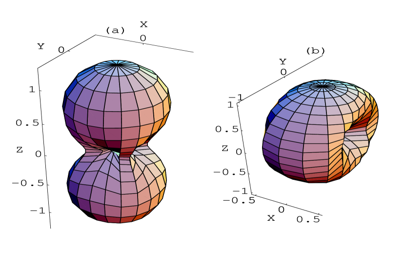
FIG. 1.: Plots of the quantity $\parallel{\sf E}\parallel^{2}$ for a two-detector network as a function of the direction to the source, with $\epsilon=0$ and $\psi=0$. In (a), the two detectors are identically oriented with arms lying in the X-Y plane, but have different noise PSDs, say $g_{(1)}=1$ and $g_{(2)}=0.25$. Whereas in (b), the two detectors have identical noise PSDs, i.e., $g_{(1)}=g_{(2)}=1$, but have different orientations, say, $\alpha_{(1)}=\beta_{(1)}=\gamma_{(1)}=0$ and $\alpha_{(2)}=\gamma_{(2)}=0$, $\beta_{(2)}=90^{\circ}$, with respect to a fide frame.

The above analysis also suggests the normalization for the network signal. The signal vector with unit norm is defined by $\hat{\sf s}\equiv{{\sf s}/{\sf b}}$. Its components are

$$\hat{s}^{I}={\Re}\left[({Q_{I}}^{*}S^{I})e^{i\delta_{c}}\right]\ \ ,$$ (55)

where

$$Q^{I}\equiv{E^{I}\over{\parallel{\sf E}\parallel}}\,.$$ (56)

Note that the network vector ${\sf Q}=(Q^{1},Q^{2},....,Q^{M})$ lies in ${\cal C}^{M}$ and has a unit norm, i.e., ${\parallel{\sf Q}\parallel^{2}}=1$.

IV Maximizing the LLR

In the case of a single detector, the LLR is a functional of the data as measured by that detector. For a network of $M$ detectors, one needs to compute the statistic in terms of the network data-vector $\sf x$. When our assumptions about the statistical properties of detector noise are valid, the appropriate network LLR is given by Eq. (28). The optimal network statistic is obtained by maximizing this LLR over the eight physical parameters that define the signal. It is this maximized LLR that must be compared with a predetermined threshold, corresponding to a given false alarm probability. In the following two subsections, we show how such a maximization over four of the parameters can be performed analytically. Subsequently, we describe an efficient way of maximizing over the time of final coalescence or, analogously, over the time of arrival (at the fide) of the signal.

A Maximizing the LLR over ${\sf b}$ and $\delta_{c}$

We begin by analytically maximizing the network LLR with respect to two parameters that are simplest to handle, namely, $r$ and $\delta_{c}$. Note that the network LLR obtained in Eq. (28) can be expressed as an explicit function of ${\sf b}$:

$$\ln\lambda={\sf b}\sum_{I=1}^{M}\langle\hat{s}^{I},x^{I}\rangle_{(I)}-{1\over 2}{\sf b}^{2}\,.$$ (57)

Above, the luminosity distance, $r$, appears only through ${\sf b}$. Maximizing $\ln\lambda$ with respect to ${\sf b}$ gives

$$\hat{\sf b}=\sum_{I=1}^{M}\langle\hat{s}^{I},x^{I}\rangle_{(I)}\ \ ,$$ (58)

where a hat denotes the value of a variable at which the LLR is a maximum as a function of that variable, keeping all other variables fixed. Here, the value of LLR at ${\sf b}=\hat{\sf b}$ is

$$\ln\lambda|_{\hat{\sf b}} = {1\over 2}\left(\sum_{I=1}^{M}\langle\hat{s}^{I},x^{I}\rangle_{(I)}\right)^{2}$$ (59)

$$= {1\over 2}\left({\Re}\left[e^{-i\delta_{c}}\left({\sf C}\cdot{\sf Q}\right)\right]\right)^{2}\ \ ,$$ (60)

where we have defined,

$$C_{I}^{*}=c_{0}^{I}-ic_{\pi/2}^{I}\equiv\langle S^{I},x^{I}\rangle_{(I)},$$ (61)

with $c_{0}^{I}=\langle s_{0}^{I},x^{I}\rangle_{(I)}$ and $c_{\pi/2}^{I}=\langle s_{\pi/2}^{I},x^{I}\rangle_{(I)}$. $C^{I}$ is a complex quantity that combines the correlations of the two quadratures of the normalized template with the data. We proceed further and maximize the LLR in (60) with respect to $\delta_{c}$. This yields,

$$\hat{\delta_{c}}=\arg\left({\sf C}\cdot{\sf Q}\right)\ \ ,$$ (62)

and the LLR maximized over ${\sf b}$ and $\delta_{c}$ as,

$$\ln\lambda|_{\hat{\sf b},\hat{\delta}_{c}}={1\over 2}\left|{\sf C}\cdot{\sf Q}\right|^{2}\,.$$ (63)

Now the maximized LLR is a function of six parameters, namely, $\{\epsilon,\psi,t_{c},\xi,\theta,\phi\}$.

When all the detectors are “closely” located or coincident, it is only the $Q^{I}$’s that depend on four angles $\{\theta,\phi,\epsilon,\psi\}$; the $C^{I}$ then depend only on $\{t_{c},\tau_{(I)},\xi\}$, with all the times of arrival being equal. We refer to this situation as the “same-site” approximation. Such a case was dealt with in Ref. [13]. When the detectors are spatially well separated or non-coincident, the $C^{I}$ depend on $\{\theta,\phi\}$ as well. In such a case, maximization over the remaining parameters is not as simple as in the same-site approximation. However, in Ref. [14] it was found that analytic maximization over two of the angular variables, $\{\psi,\epsilon\}$, is possible even in the case of non-coincident detectors. This useful observation allowed further reduction of the LLR to obtain a network statistic. In the following, we briefly mention this analytic maximization before discussing how the reduced statistic can be used for searching chirps.

B Further maximization over $\epsilon$ and $\psi$

For spatially separated detectors the cross-correlation, $C^{I}$, is strongly dependent on the time of final coalescence, ${t_{c}}$, and the time delay, $\tau_{(I)}$. Since $\tau_{(I)}$ depends on the source-direction, $(\theta,\phi)$, so does $C^{I}$. This prompts us to recast the statistic, (63), in such a way that its dependence on the angles $\{\psi,\epsilon\}$ is isolated as shown below. This aids in the analytic maximization of $\ln\lambda|_{\hat{\sf b},\hat{\delta_{c}}}$ over the angles $\{\epsilon,\psi\}$. We note that using Eqs. (48) and (56), the network vector $\sf Q$ can be re-expressed as

$${\sf Q} = {1\over{\parallel{\sf E}\parallel}}\left[T_{2}{}^{-2}(\psi,\epsilon,0){\sf D}_{-2}+T_{2}{}^{2}(\psi,\epsilon,0){\sf D}_{+2}\right]$$ (64)

$$\equiv Q^{-2}{\hat{\sf D}}_{-2}+Q^{+2}{\hat{\sf D}}_{+2}\ \ ,$$ (65)

where ${\sf D}_{p}$ ($p=\pm 2$) define two network vectors with the components $g_{(I)}{D}^{I}_{p}$, respectively. The vectors ${\hat{\sf D}}_{p}$ are their normalized counterparts. Since ${\sf Q}$ has a unit norm, the above expression implies that

$$Q^{-2}={{\parallel{\sf D}\parallel}\over{\parallel{\sf E}\parallel}}T_{2}{}^{-2}(\psi,\epsilon,0),\hskip 21.68121ptQ^{+2}={{\parallel{\sf D}\parallel}\over{\parallel{\sf E}\parallel}}T_{2}{}^{2}(\psi,\epsilon,0)\ \ ,$$ (66)

where ${\parallel{\sf D}\parallel}\equiv{\parallel{{\sf D}_{+2}}\parallel}={\parallel{{\sf D}_{-2}}\parallel}$.

The following relations hold among $Q^{\pm 2}$, $Q_{\pm 2}$, and ${\hat{\sf D}}_{\pm 2}$:

$$Q_{+2} \equiv {\hat{\sf D}}_{+2}\cdot{\sf Q}=Q^{+2}+Q^{-2}{\hat{\sf D}}_{+2}\cdot{\hat{\sf D}}_{-2}\ \ ,$$ (67)

$$Q_{-2} \equiv {\hat{\sf D}}_{-2}\cdot{\sf Q}=Q^{+2}{\hat{\sf D}}_{-2}\cdot{\hat{\sf D}}_{+2}+Q^{-2}\,.$$ (68)

The pair $\{{\hat{\sf D}}_{+2},{\hat{\sf D}}_{-2}\}$ defines a two-dimensional complex subspace in ${\cal C}^{M}$, on which a metric $G_{pq}$ can be defined. ${\hat{\sf D}}_{+2}$ and ${\hat{\sf D}}_{-2}$ depend only on the direction of the source and the orientation of the detectors, that is, on $\{\theta,\phi,\alpha_{(I)},\beta_{(I)},\gamma_{(I)}\}$ and not on $\{\epsilon,\psi\}$. The metric components in the ${\hat{\sf D}}_{\pm 2}$ basis are given by,

$${{G_{pq}}=\left(\begin{array}[]{ccc}1&{\hat{\sf D}}_{+2}\cdot{\hat{\sf D}}_{-2}\\ {\hat{\sf D}}_{-2}\cdot{\hat{\sf D}}_{+2}&1\end{array}\right)\,.}$$ (69)

This metric can be used to ‘raise’ and ‘lower’ indices of vectors lying in this complex subspace, e.g., one has $Q_{p}=G_{pq}Q^{q}$, where $p$, $q=\pm 2$. We observe that, in general, ${\hat{\sf D}}_{\pm 2}$ are not orthogonal. For a face-on binary (i.e., $\epsilon=0$) revolving anti-clockwise (or clockwise), ${\sf D}_{p}$ itself is proportional to the network vector ${\sf E}$ for $p=-2$ (or for $p=2$). Hence, we may call the two-dimensional subspace as the “helicity” plane, ${\cal H}$.

The $M$-dimensional complex correlation vector ${\sf C}$, in general, lies outside ${\cal H}$. However, ${\sf Q}$ lies totally in ${\cal H}$. Thus, the statistic reduces to

$$2\ln\lambda|_{\hat{\sf b},\hat{\delta}_{c}}=\left|{\sf C}\cdot{\sf Q}\right|^{2}=\left|{\sf C}_{\cal H}\cdot{\sf Q}\right|^{2}\ \ ,$$ (70)

where ${\sf C}_{\cal H}$ is the projection of ${\sf C}$ on ${\cal H}$. Maximization of the above statistic over $\{\epsilon,\psi\}$ is achieved by aligning ${\sf Q}$ along ${\sf C}_{\cal H}$ by a proper choice of $\psi$ and $\epsilon$. To show that this is always possible, we expand ${\sf C}_{\cal H}$ in the two-dimensional basis $({\hat{\sf D}}_{+2},{\hat{\sf D}}_{-2})$:

$${\sf C}_{\cal H}=C^{-2}_{\cal H}{\hat{\sf D}}_{-2}+C^{+2}_{\cal H}{\hat{\sf D}}_{+2}\ \ ,$$ (71)

where $C^{p}_{\cal H}\equiv G^{pq}({\hat{\sf D}}_{q}\cdot{\sf C})$. Then the maximization condition is

$${{Q^{+2}}\over{Q^{-2}}}={{C^{+2}_{\cal H}}\over{C^{-2}_{\cal H}}}\,.$$ (72)

In principle, ${\sf C}$ can take any value in ${\cal C}^{M}$, so the RHS of (72) can take any value in the complex plane. The task is to prove that the ratio ${{Q^{+2}}/{Q^{-2}}}$ obeys the same property. In other words, we must show that the ratio ${{Q^{+2}}/{Q^{-2}}}$ too can span the entire complex plane. This follows immediately from the observation that

$${Q^{+2}\over{Q^{-2}}}={{T_{2}{}^{-2}(\psi,\epsilon,0)}\over{T_{2}{}^{2}(\psi,\epsilon,0)}}=\left({{1-\cos\epsilon}\over{1+\cos\epsilon}}\right)^{2}\exp({4i\psi})\,.$$ (73)

For $\epsilon\in[0,\pi]$ and $\psi\in[0,2\pi]$, the RHS of (73) can indeed attain any value in the Argand plane. One set of values of $\hat{\psi}$ and $\hat{\epsilon}$ that maximizes the statistic are

$${\hat{\psi}}={\arg(\zeta)\over 4},\hskip 21.68121pt{\hat{\epsilon}}=\cos^{-1}\left[{1-\sqrt{|\zeta|}}\over{1+\sqrt{|\zeta|}}\right]\ \ ,$$ (74)

where $\zeta\equiv C^{+2}_{\cal H}/C^{{-2}}_{\cal H}$. Thus, the LLR maximized over the four parameters is

$$2\ln\lambda|_{{\hat{\sf b}},{\hat{\delta}_{c}},{\hat{\psi}},{\hat{\epsilon}}}={\parallel{\sf C}_{\cal H}\parallel}^{2}\equiv\Lambda\,.$$ (75)

Geometrically, we summarize the above maximization over the angles $\{\epsilon,\psi\}$ as follows: Choosing a given source direction fixes the orientation of the helicity plane in the network space. After making this choice, one projects the correlation vector ${\sf C}$ onto this plane. The vector ${\sf Q}$ inevitably lies in this plane. Thus, the values of $\{\epsilon,\psi\}$ that maximize the statistic are those that align the vector ${\sf Q}$ along the projected vector ${\sf C}_{\cal H}$.

It is always possible to choose in ${\cal H}$, a two-dimensional basis comprising of a pair of orthonormal real vectors. In such a basis the components of any vector in ${\cal H}$ will, in general, be complex. For the sake of concreteness, we define one such basis, $({\hat{\sf v}}^{+},{\hat{\sf v}}^{-})$, in the following way. We split ${\sf D}_{+2}$ into its real and imaginary parts

$${\sf D}_{+2}\equiv{\sf d}_{1}+i{\sf d}_{2}\ \ ,$$ (76)

where ${\sf d}_{1}$ and ${\sf d}_{2}$ are real vectors. We then define

$${\hat{\sf v}}^{\pm}=({\hat{\sf d}}_{1}\pm{\hat{\sf d}}_{2})/\parallel{\hat{\sf d}}_{1}\pm{\hat{\sf d}}_{2}\parallel\,.$$ (77)

Taking the projection of ${\sf C}$ on ${\hat{\sf v}}_{\pm}$, i.e., $C^{\pm}\equiv{\hat{\sf v}}^{\pm}\cdot{\sf C}=c_{0}^{\pm}+ic_{\pi/2}^{\pm}$, we re-express Eq. (75) as

$${\parallel{\sf C}_{\cal H}\parallel}^{2} = {|{C}^{+}|}^{2}+{|{C}^{-}|}^{2}=(c_{0}^{+})^{2}+(c_{\pi/2}^{+})^{2}+(c_{0}^{-})^{2}+(c_{\pi/2}^{-})^{2}$$ (78)

$$\equiv \L^{2}\,.$$ (79)

It can be verified that the statistic is, therefore, a sum of the squares of four Gaussian random variables with constant variance. With an appropriate choice of normalization, these variances can be made unity. As we show in Sec. VII, this simplifies the computation of detection thresholds and probabilities associated with the above statistic. Instead of using the squared norm of $\sf{C}_{\cal H}$, we will find it convenient to use as our statistic $\L\equiv\parallel{\sf C}_{\cal H}\parallel$, in what follows. We note that $\L$ then scales linearly with the amplitude of the signal vector, rather than its square. We will call $\L$ as our network statistic. This statistic was first obtained in Ref. [14].

C Maximizing $\L$ over the time of arrival

Given a network data-vector, ${\sf x}(t)$, which may or may not contain a chirp, it is necessary to first compute the correlation vector, ${\sf C}$, before one can obtain ${\sf C}_{\cal H}$ and, therefore, the network statistic. In order to do so, we need $C^{I}$, for all $I$. We compute a $C^{I}$ (or, rather, $C_{I}^{*}$) by first calculating the Fourier transform of the cross-correlation (61) for an individual detector by using FFTs. Taking its inverse FFT then gives us the $C_{I}^{*}(\tau)$ at all the time lags, $\tau$, in a cost effective way. Thus we get,

$$C_{I}^{*}(\tau;t^{\prime}_{c},\xi^{\prime},\theta^{\prime},\phi^{\prime})=\langle S^{I}(t;t^{\prime}_{c}+\tau,\xi^{\prime}),x^{I}(t;t_{c},\xi)\rangle_{(I)}\ \ ,$$ (80)

where the primed parameters define the detector template. If the values chosen for $\{\xi^{\prime},\theta^{\prime},\phi^{\prime}\}$ match those of a chirp in the data, then $|C^{I}|$ is likely to peak when $\tau$ exactly compensates for the difference $(t^{\prime}_{c}-t_{c})$. Indeed, the correct ${\sf C}$ for a network of coincident detectors is just

$${\sf C}(\tau;\mbox{\boldmath$\vartheta$}^{\prime})\equiv\{C^{I}(\tau;\mbox{\boldmath$\vartheta$}^{\prime})\}\ \ ,$$ (81)

where $\mbox{\boldmath$\vartheta$}^{\prime}$ is the four-dimensional template parameter-vector. Also, $I$ takes values from $1$ to $M$.

Construction of ${\sf C}$ for a network of non-coincident detectors is somewhat more involved owing to non-vanishing time-delays, $\tau_{(I)}(\theta,\phi)$, that may arise for a given source direction. Recall that the time of arrival at the $I$-th detector is $t_{a}+\tau_{(I)}(\theta,\phi)$. If the detectors are spread around the globe, the times of arrival at any pair of detectors can at most differ by $2R_{\oplus}/c\sim 40$ ms, where $R_{\oplus}$ is the radius of the Earth. For the two LIGO detectors, the maximum time difference is $\sim 10$ ms; for the network of LIGO-VIRGO, it is $\sim 27$ ms. We note that $\tau_{(I)}(\theta,\phi)$ can take positive as well as negative values. Its range depends on the location of the fide. If the fide is chosen at the center of the Earth, then $|\tau_{(I)}|\leq R_{\oplus}/c$; but if it is chosen to be one of the detectors on the surface of the Earth, then $|\tau_{(I)}|\leq 2R_{\oplus}/c$. This contingency is dealt with by using the appropriate set of $\tau_{(I)}$’s in Eq. (38) to obtain the $S^{I}(t;t^{\prime}_{c},\xi^{\prime})$. With this in place, the network correlation-vector is given by the same expression as in Eq. (81).

One can obtain the same value for ${\sf C}$ by an alternative construction, which may be simpler to implement in practice. In this method, one first obtains the $S^{I}$ by setting the arrival time at every detector to equal that at the fide. This is the same as computing the $S^{I}(t+\tau_{(I)};t^{\prime}_{c},\xi^{\prime})$, for all $I$. (Note from Eq. (38) that, despite appearances, a knowledge of $\tau_{(I)}$’s is actually not needed for this computation.) With these templates one constructs the following inner products:

$$\bar{C}_{I}^{*}(\tau;t^{\prime}_{c},\xi^{\prime})\equiv\langle S^{I}(t+\tau_{(I)};t^{\prime}_{c}+\tau,\xi^{\prime}),x^{I}(t;t_{c},\xi)\rangle_{(I)}\ \ ,$$ (82)

which are independent of the time delays. Indeed, a choice of the time delays is not made thus far in this alternative construction of ${\sf C}$. To construct the network correlation-vector from the above quantities, one begins by choosing a source direction, $\{\theta^{\prime},\phi^{\prime}\}$, for the template. This direction is used to compute a consistent set of time delays, $\tau_{(I)}(\theta^{\prime},\phi^{\prime})$, for a given network. The network correlation-vector can then be defined as

$${\sf C}(\tau;\mbox{\boldmath$\vartheta$}^{\prime})=\{\bar{C}^{I}(\tau+\tau_{(I)}(\theta^{\prime},\phi^{\prime});t^{\prime}_{c},\xi^{\prime})\}\ \ ,$$ (83)

where the appropriately shifted time lags for each value of $I$ compensates for the time-delay at each detector. In the rest of this section, we discuss the construction of network templates in greater detail. There, for a network of non-coincident detectors, we choose this latter prescription for such a construction.

Network template construction

Based on the above discussion, we construct a network template as follows. Given a chirp, consider the detector with the least seismic cut-off frequency. Label that detector as $I=1$. The other detectors in the network are labeled such that $f_{s(1)}\leq f_{s(2)}\leq\cdots f_{s(M)}$. Then from Sec. III we have ${\xi}_{(1)}\geq{\xi}_{(2)}\geq\cdots{\xi}_{(M)}$. Now, consider the signal in the first detector, $I=1$. It lasts $\xi_{(1)}$ seconds. As in the case of a single-detector “network”, an individual detector template, which is an array of numbers, is constructed to be much longer than the signal: It comprises of a sub-array that stores the signal being searched for, followed by a padding of the requisite number of zeros [28]. In the single-detector case, it has been shown that a padding factor of $75\%$, that is, $75\%$ zeros and $25\%$ signal, is a good choice in the sense that it optimizes the computational cost arising from the computation of the FFT’s. Accordingly, here too we pad the template for the first detector with zeros for a time duration of $\sim 3\xi_{(1)}$.

In the sensitivity window of any of the other detectors, that is, for $(I\neq 1)$, the signal effectively lasts for a time-duration equal to or shorter than $\xi_{(1)}$. Nevertheless, the simplest way to construct their templates is to let them contain the same signal as in the first detector, and for the same duration, namely, $\xi_{(1)}$. Such a construction does not restrict the network statistic in any way. Its only pertinent implication is that any part of the signal that has an instantaneous frequency below $f_{s(I)}$ will be ineffective in contributing to the SNR in the $I$-th detector, which conforms with what we expect. In the case of a network with coincident detectors, the individual detector-templates so constructed define the components of the network template-vector. Using it in Eq. (81) yields the relevant network correlation-vector.

Obtaining the template-vector of a network with non-coincident detectors is trickier. This is essentially due to the possibility of the occurrence in a given detector of negative time-delays. We deal with this possibility by splitting the padding into two parts of durations $\tau_{d}$ and $(3\xi_{(1)}-\tau_{d})$, respectively. Since the maximum magnitude that a time-delay can have is less than $50$ ms, a choice of $\tau_{d}=50$ ms satisfies all requirements at negligible cost. This is the value we assume for $\tau_{d}$ in our simulations. Thus, the template of any one of the detectors in such a network is an array of numbers that begins with a “pre-padding” (with zeros) of duration $\tau_{d}$ preceding the signal of interval $\xi_{(1)}$, which in turn is followed by a “post-padding” of duration $(3\xi_{(1)}-\tau_{d})$. The network template is then the Cartesian product of all these individual templates. Note that this can be taken to define the network template for the most general network, regardless of whether the detectors in it are coincident or not. For non-coincident detectors, the relative time-delays are accounted for in the construction of the network statistic via Eq. (83).

In order to construct the network correlation-vector, ${\sf C}$, one utilizes the above templates as follows. Using these individual-detector templates one first obtains the correlations $\bar{C}^{I}(\tau;t^{\prime}_{c},\xi^{\prime})$ for all values of $\tau$ (after setting $t^{\prime}_{a}=0$ or, equivalently, $t^{\prime}_{c}=\xi^{\prime}$, without any loss of generality) by using the FFT algorithm, such as in the single-detector case. Note that the range of $\tau$, for a data train of length $T$, is $\tau_{d}\leq\tau\leq T-\xi_{(1)}-\tau_{d}$. Next one selects a source direction, $(\theta^{\prime},\phi^{\prime})$. One evaluates the time-delays, $\tau_{(I)}(\theta^{\prime},\phi^{\prime})$, corresponding to this direction. These time delays are then used in Eq. (83) to compute ${\sf C}$, which in turn is projected on ${\cal H}$ (defined by the same selection of $\{\theta^{\prime},\phi^{\prime}\}$) in order to obtain ${\sf C}_{\cal H}$. The network statistic can be easily recovered from this using Eq. (75).

In Fig. 2 (a), we show a network template for a network of two detectors. In all the panels, the dots represent the padding (with zeros), which is introduced before and after the signal. The two panels in (a) depict the two individual detector-templates constituting the network template. These two panels correspond to detectors with different seismic cut-offs, viz., $f_{s(1)}=33$ Hz and $f_{s(2)}=40$ Hz, respectively. The padding before (i.e., on the left-hand side of) the signal is of a duration $\tau_{d}=50$ ms. The part of the curve for detector 2 that is shown in dots and dashes is ineffective in contributing to the SNR. Panels (b) show the relative positions of the signal in the individual detector-templates for which $\|{\sf C}\|$ has a maximum when the second detector has a relative time-delay of $(\tau_{(2)}-\tau_{(1)})=20$ ms. Here, we have included the time delay in the network template.

Above, the chirp time in the detector with the least $f_{s(I)}$ decided the durations of the padding and the chirp-signal in all the individual detector-templates. Indeed, these durations are the same in all of them. It may be possible to optimize on computational costs by varying these durations in different templates. However, in this work we do not pursue this point any further.

FIG. 2.: Network template for a two-detector network. We choose the fiducial frequency as $f_{s}=40$ Hz. The instant at which the signal reaches $f_{s}$ is shown by a vertical line. We take the chirp time corresponding to the fide to be $\xi=0.3$ sec. The dots represent the padding with zeros, which is introduced before and after the signal. The two panels in (a) depict the two individual detector-templates constituting the network template. These two panels correspond to detectors with different seismic cut-offs, viz., $f_{s(1)}=33$ Hz and $f_{s(2)}=40$ Hz, respectively. The respective chirp times are $\xi_{(1)}=0.5$ sec and $\xi_{(2)}=0.3$ sec. The padding before (i.e., on the left-hand side of) the signal is of a duration $\tau_{d}=50$ ms. The part of the curve for detector 2 that is shown in dots and dashes is ineffective in contributing to the SNR. Panels (b) show the relative positions of the signal in the individual detector-templates for which $\|{\sf C}\|$ has a maximum when the second detector has a relative time-delay of $(\tau_{(2)}-\tau_{(1)})=20$ ms. Each of the detectors has its seismic cut-off equal to $40$ Hz, which gives $\xi_{(1)}=\xi_{(2)}=\xi=0.3$ sec.

D Maximization of $\L$ over $\xi$, $\theta$, and $\phi$.

Consider the network correlation-vector, ${\sf C}(\tau)$, for a fixed value of $\xi^{\prime}$, but for a range of values for $\tau$. As remarked before, such a vector is constructed for specific values of $\tau$ and source direction $(\theta^{\prime},\phi^{\prime})$ by taking into account the time delays, $\tau_{(I)}(\theta^{\prime},\phi^{\prime})$, appropriate for the network under consideration. The network statistic for these chosen values of $(\theta^{\prime},\phi^{\prime})$ and $\tau$ can be obtained by first projecting ${\sf C}$ on the helicity plane and then computing the norm of the projection. A chirp search over $\{\theta^{\prime},\phi^{\prime}\}$ for a given configuration of network leads to a “window” of time delays. In any network of non-coincident detectors a window, $W$, is a bounded region in the space of time-delays that arises from the restrictions on each of the time delays to lie within certain limits. As we illustrate below, these limits, in turn, originate owing to the maximum light-travel time between pairs of detectors. Since the data are sampled discretely, a window is a bounded region of a lattice in the space of possible time-delays. Consequently, the number of (lattice) points in a window of finite “volume” is also finite. We now discuss the shape and size of a window for networks with two, three, four, and more than four detectors.

• Two-detector network:
  For a network of two detectors, there exists effectively a single time-delay function of significance. It is the difference in the times of arrival of the wave at the two detectors. For such a network we choose one of the detectors, say, $I=1$, as the fide. Then $\tau_{(1)}=0$ and the time delay between the two detectors is reflected solely in $\tau_{(2)}$, which is restricted to lie within the range $[-d_{12}/c,d_{12}/c]$, where $d_{12}$ is the distance between the two detectors. Let $\Delta$ be the sampling interval, which is typically $0.5$ ms. Then the “width” of the window, expressed in terms of the number of time-sampled points, is $n_{S}^{\Omega}=2\tau_{(2)}/\Delta$, where the subscript $S$ stands for sampling and $\Omega$ for the direction in sky, $(\theta,\phi)$. If we denote the LIGO detector at Hanford by H, the LIGO detector at Louisiana by L, and the VIRGO detector by V, then for the two-detector networks formed from pairs among these, we have $n_{S}^{\Omega}$($LH$) $\sim 40$, $n_{S}^{\Omega}$($HV$) $\sim 108$, and $n_{S}^{\Omega}$($LV$) $\sim 105$.

• Three-detector network:
  In the case of a network with three detectors, we once again take the first one (i.e., $I=1$) to be fiducial. Also, we can always imagine all of them to lie on a single plane. In such a case, there arise two nontrivial time-delays, namely, $\tau_{(2)}$ and $\tau_{(3)}$. The allowed values of these two time-delays are easily shown to be restricted within a bounded region of a plane; this region is circumscribed by an ellipse. Any point in this region represents a pair of time-delay values, $(\tau_{(2)},\tau_{(3)})$, corresponding to a given pair of values for the source-direction angles, $\{\theta^{\prime},\phi^{\prime}\}$. The equation of this ellipse is given by [7]

  $$(\tau_{(2)})^{2}+(\tau_{(3)})^{2}(p^{2}+q^{2})-2p\tau_{(2)}\tau_{(3)}-q^{2}(d_{12}/c)^{2}=0\ \ ,$$ (84)

  where $p=(d_{13}/d_{12})\cos{\alpha_{23}}$ and $q=(d_{13}/d_{12})\sin{\alpha_{23}}$, with $d_{12}$ (or $d_{13}$) being the distance between the first and the second (or third) detectors. Also, ${\alpha_{23}}$ is the angle subtended by the hubs of detectors 2 and 3 at that of the first detector. From (84), the “area” of the elliptical window, given in terms of the number of time-sampled points, is $n_{S}^{\Omega}=2\pi\times{\cal A}/(c^{2}\Delta^{2})$ where $\cal A$ is the area of the triangle formed by the hubs of the three detectors in the network. We find that the number of possible time-delays for the three-detector network of LIGOs-VIRGO ($LHV$) is $n_{S}^{\Omega}\sim 3\times 10^{3}$.

• Four and more detectors:
  In the case of a three-detector network, the two time-delays produce two circles on the celestial sphere that intersect at two points, which give the possible directions to the source. This two-fold degeneracy is broken when we introduce a fourth detector lying outside the plane of the three detectors. In such a case, the possible time-delays can be represented in a three-dimensional space of the three time-delays, which now lie on the surface of an ellipsoid. The number of possible time-delays is exactly doubled compared to that of the three-detector network. Thus, its maximum possible value is $n_{S}^{\Omega}=4\pi{\cal A}/(c^{2}\Delta^{2})$, where ${\cal A}$ is the area of the smallest of all possible triangles formed subsets of three of the four detectors. When there are more than 4 detectors there is redundant information on the direction to the source, but the $n_{S}^{\Omega}$ is the same as for four detectors. In the presence of noise this redundant information may be used to reduce the errors in the direction to the source. Here, we do not pursue this point any further.

The sampling interval naturally provides the most simplistic discretization in carrying out the search in time-delays. In searching over $\theta$ and $\phi$ one does not need to compute additional Fourier transforms; rather, one needs to combine the individual detector-correlations with the correct time delays to construct the optimal statistic, $\L$. This gives rise to two components to the computational cost: the cost involved in computing Fourier transforms and the cost arising due to the arithmetic operations involved in computing $\L$ over all possible time-delays. As shown later, the latter cost can be considerable and may dominate over the cost in computing Fourier transforms while searching over $\xi$.

It is important to note that sampling can introduce an arbitrary mismatch between the actual source direction, $(\theta$, $\phi)$, and the direction in the template, $(\theta^{\prime}$, $\phi^{\prime})$. The mismatch, $\mu$, is the fractional loss in SNR when the signal and the template parameter differ slightly. In agreement with most investigations carried out so far, we decide to tolerate a mismatch to a maximum of $3\%$. The sampling can lead to a mismatch either greater or smaller than $\mu$. If the sampling gives a mismatch less than the desired one, then this simplistic procedure of scanning $W$ leads to unnecessary extra computational costs. On the other hand, if the mismatch is more, then one is likely to miss out more events than desired. The question whether the sampling is adequate one way or the other can be resolved by constructing a template-bank for the desired mismatch $\mu$. In the next section, we proceed to construct a bank of templates in the parameter $\xi$, $\theta$, and $\phi$. The template bank, in general, will produce time-delays that do not fall exactly at the sampled values of the correlation vector. However, we can easily interpolate to obtain the intermediate values by applying Shannon’s theorem [29], which essentially states that a band-limited function can be constructed in the time domain from its discretely sampled values at the Nyquist rate. Or in other words, the template bank provides the rate at which the output can be re-sampled so as to obtain the desired maximum mismatch.

V Template bank in $\xi$, $\theta$, and $\phi$

Recall that the LLR is a function of eight parameters, namely $\{r,\delta_{c},\epsilon,\psi,t_{c},\xi,\theta,\phi\}$ for the Newtonian chirp. As mentioned earlier, we adopt the maximum-likelihood method for the detection problem. It implies that the LLR must be maximized over all the parameters to obtain the MLR. We have shown that the maximization of LLR can be carried out analytically with respect to the four of the eight parameters, $\{r,\delta_{c},\epsilon,\psi\}$. Also, we can deal with the time of final coalescence at the fide $t_{c}$ efficiently by using the FFT algorithm. Therefore, we now need to formulate a strategy to search over the rest of the 3-D parameter space formed by $\xi$, $\theta$, and $\phi$. Ideally, one should scan the whole range of the 3-D parameter space over the physically allowed parameter values. This, however, is impractical due to computational limitations. Therefore, a prerequisite for such a maximization is an estimate for the magnitude of grid discretization. The grid spacing in the parameter space depends upon the fractional loss in the SNR that one is prepared to tolerate.

To estimate the number of templates in the 3-D parameter space, we take the differential-geometric approach [30] and use Owen’s method of introducing a metric on that space [23] and extend his formula for the one detector case to that of the network. Also the inverse of the metric is just the covariance matrix scaled by the square of the SNR. Thus the metric also provides information on the errors in estimating the parameters. In this geometric method, the signal vector is characterized by $P+1$ parameters, $\vartheta^{\alpha}$, where $\alpha=0,1,...,P$. The signal vector lies in a $(P+1)$-dimensional manifold denoted by ${\cal P}$. We define the metric on $\cal{P}$ by $g_{\alpha\beta}$, which is related to the fractional loss in SNR, denoted by $\mu$, when there is a mismatch between the signal and the template parameters. Since here we consider the Newtonian chirp as our signal, we have $P=3$, $\vartheta^{0}\equiv t_{c}$, and $\vartheta^{i}\equiv\{\xi,\theta,\phi\}$. As $\L$ can be maximized over $t_{c}$ numerically via the FFT, we only need to lay the templates in the rest of the $P$-dimensional parameter space, comprising of $\{\xi,\theta,\phi\}$. In other words, we need to compute the metric $\gamma_{ij}$ in the $P$-dimensional subspace. It is determined by projecting the metric $g_{\alpha\beta}$ onto the subspace orthogonal to $t_{c}$. We then obtain

$$\gamma_{ij}=g_{ij}-{{g_{0i}g_{0j}}\over{g_{00}}}\,.$$ (85)

The number of templates is obtained as follows. We compute the proper volume of the parameter space with the metric $\gamma_{ij}$ and multiply the volume by the number density of the templates. Fixing the value of $\mu$ determines the grid spacing of the network templates in the parameter space. The number density, $\rho_{P}(\mu)$, which is the number of templates per unit proper volume, is given by

$$\rho_{P}(\mu)=\left({1\over 2}\sqrt{P\over\mu}\right)^{P}\,.$$ (86)

It is defined to be uniform over the whole parameter space and, therefore, its use is applicable as long as the curvature of the astrophysically interesting region of the manifold described by $\gamma_{ij}$ is sufficiently small, and the effects arising from the boundary of the region are negligible.

The total volume of the parameter space is

$${\cal V}=\int_{\cal P}\sqrt{\det\parallel\gamma_{ij}\parallel}\hskip 7.22743ptd^{P}\vartheta\,.$$ (87)

Thus, the total number of templates required is , $n_{f}={\cal V}\times\rho_{P}(\mu)$ . In general, the total number of templates depends on the source parameters $\{\epsilon,\psi\}$. In order to scan the parameter space (for a given mismatch $\mu$) for each pair of values $\{\epsilon,\psi\}$, we must maximize the volume ${\cal V}$ over $\{\epsilon,\psi\}$. This is tantamount to choosing the finest bank of templates. For simple cases, this is straightforward and has been implemented in some examples in Sec. VI. In general, however, such a maximization is non-trivial to perform.

A The network metric

We apply the method described above to obtain the metric in the four-dimensional parameter space $\{t_{c},\xi,\theta,\phi\}$. When the parameters of the network template and that of signal mismatch, the network statistic given by (78) drops below the maximum value. The metric $g_{\alpha\beta}$ defined on this four-dimensional space is related to the amount of drop in the statistic, ${\L}$, and is obtained by expanding the statistic about the maximum. Using Eq. (78) the squared statistic can be rewritten as,

$$\L^{2} = |{\hat{\sf v}}^{+^{\prime}}\cdot{\sf C}|^{2}+|{\hat{\sf v}}^{-^{\prime}}\cdot{\sf C}|^{2}$$ (88)

$$\equiv p^{\prime}_{I}{}^{J}C^{I}C_{J}^{*}\,.$$ (89)

The quantity $p^{\prime}_{I}{}^{J}$ is a projection tensor given by,

$$p^{\prime}_{I}{}^{J}\equiv{v^{\prime}}^{+J}{v^{\prime}}^{+}_{I}+{v^{\prime}}^{-J}v^{\prime-}_{I}\ \ ,$$ (90)

which projects a vector in ${\cal C}^{M}$ on the helicity plane spanned by ${\hat{\sf v}}^{\prime\pm}$. It obeys the identities

$$p^{\prime}_{I}{}^{J}p^{\prime}_{J}{}^{K}=p^{\prime}_{I}{}^{K}\>,\hskip 36.135ptp^{\prime}_{I}{}^{J}p^{\prime}_{J}{}^{I}=2\ \ ,$$ (91)

which are consistent with its being a projection tensor on a two-dimensional plane. The primed coordinates refer to the template.

Let $\vartheta^{\alpha}$ and $\vartheta^{\prime\alpha}=\vartheta^{\alpha}+\Delta\vartheta^{\alpha}$ be the parameters corresponding to the signal and the network template, respectively. For computing the metric one takes normalized templates for the signal as well as the template, so that the maximum value of $\L$ is unity when the parameters of the signal and template match. In the absence of noise, Eq. (61) yields

$$C_{I}^{*}=\langle S^{\prime I},s^{I}\rangle_{(I)}\simeq e^{i\delta_{c}}Q_{I}^{*}\langle S^{\prime I},S^{I}\rangle_{(I)}\ \ ,$$ (92)

where, the $S^{\prime I}$ denotes the template. The above expression is exact within the SPA. So the statistic can be written as,

$$\L^{2}=p^{\prime}_{I}{}^{J}Q^{I}Q_{J}^{*}\Theta_{(I)(J)}\ \ ,$$ (93)

where

$$\Theta_{(I)(J)} \equiv \langle S^{I}(t;\vartheta^{\prime\mu}),S^{I}(t;\vartheta^{\mu})\rangle^{*}_{(I)}\langle S^{J}(t;\vartheta^{\prime\mu}),S^{J}(t;\vartheta^{\mu})\rangle_{(J)}\ \,$$ (94)

$$= \int_{f_{s(I)}}^{\infty}\!df{\cal A}_{(I)}(f)\exp\left(-i\Phi_{(I)}(f;\vartheta^{\mu},\Delta\vartheta^{\mu})\right)\int_{f_{s(J)}}^{\infty}\!df{\cal A}_{(J)}(f)\exp\left(i\Phi_{(J)}(f;\vartheta^{\mu},\Delta\vartheta^{\mu})\right)$$ (95)

is the product of the individual ambiguity functions of the $I$-th and $J$-th detectors. It is a measure of how distinguishable the two wave-forms, i.e., the signal and the template, are. Here,

$${\cal A}_{(I)}(f)\equiv{8\over{3f_{s}g_{(I)}^{2}}}{1\over{s_{h(I)}(f)}}\left({f\over f_{s}}\right)^{-7/3}\ \ ,$$ (96)

which satisfies the normalization condition $\int_{f_{s(I)}}^{\infty}{\cal A}_{(I)}(f)df=1$. Note that in the limit of $\Delta\theta^{\alpha}\rightarrow 0$ the projection tensor of the filter is same as that of the projection tensor of the signal, i.e. $p^{\prime}_{I}{}^{J}\rightarrow p_{I}{}^{J}$. In this limit, the projection tensor of the signal obeys the relation $p_{I}{}^{J}Q^{I}Q_{J}^{*}=1$ and noting that $S^{I}$’s are normalized to unity, we can see from Eq. (93) that $\L^{2}\rightarrow 1$ as desired.

The correlation phase, $\Phi_{(I)}(f;\vartheta^{\mu},\Delta\vartheta^{\mu})$, is given by (see Eq. (42)):

$$\Phi_{(I)}(f;\vartheta^{\mu},\Delta\vartheta^{\mu})=\Psi_{(I)}(f;f_{s},t_{c},\xi)-\Psi_{(I)}(f;f_{s},t^{\prime}_{c},\xi^{\prime})\,.$$ (97)

The correlation phase includes the contribution from the differential time-delay between the signal and the template. Instead of using $(\theta,\phi)$ to specify the direction to the source we use the components $n_{1}$ and $n_{3}$ of the unit vector ${\hat{\sf n}}\equiv(n_{1},n_{2},n_{3})$ to do so. The time delays in units of $f_{s}^{-1}$ are,

$$f_{s}\tau_{(I)}(n_{3},n_{1})=\left[r_{(I)1}n_{1}+r_{(I)2}(1-n_{3}^{2}-n_{1}^{2})^{1/2}+r_{(I)3}n_{3}\right]\ \ ,$$ (98)

where ${\sf r}_{(I)}$ is the position vector of the $I$-th detector’s hub and is henceforth measured in units of the “fiducial wavelength”, $\lambda_{s}\equiv c/f_{s}$. Since we choose to measure the time delays with respect to the fide, we must have ${\sf r}_{(f)}=0$. Thus, we may write the correlation phase as

$$\Phi_{(I)}(f;\vartheta^{\mu},\Delta\vartheta^{\mu})\equiv 2\pi\varphi_{(I)\alpha}(f;\vartheta^{\mu})\Delta\vartheta^{\alpha}\ \ ,$$ (99)

where $\vartheta^{\alpha}\equiv\{f_{s}t_{c},\>f_{s}\xi,\>n_{3},\>n_{1}\}$ is a quartet of dimensionless parameters and

$${\varphi_{(I)\alpha}(f;\vartheta^{\alpha})=\left\{\left({f\over f_{s}}\right),\>{3\over 5}\left({f\over f_{s}}\right)^{-5/3}\!\!\!\!,\>\left[r_{(I)3}-r_{(I)2}{{n_{3}}\over{\left(1-n_{3}^{2}-n_{1}^{2}\right)^{1/2}}}\right]{f\over f_{s}},\>\left[r_{(I)1}-r_{(I)2}{{n_{1}}\over{\left(1-n_{3}^{2}-n_{1}^{2}\right)^{1/2}}}\right]{f\over f_{s}}\right\}\,.}$$ (100)

To obtain $g_{\alpha\beta}$ we Taylor expand the network statistic about the peak at $\Delta\vartheta^{\mu}=0$ to obtain

$$\L(\mbox{\boldmath$\vartheta,\Delta\vartheta$})\approx 1+{1\over 2}{\left({{\partial^{2}{\L}}\over{\partial\Delta\vartheta^{\alpha}\partial\Delta\vartheta^{\beta}}}\right)}\Bigg{|}_{\Delta\mbox{\boldmath$\vartheta$}=0}\Delta\vartheta^{\alpha}\Delta\vartheta^{\beta}\ \ ,$$

where $\vartheta$ is the four-dimensional signal parameter-vector. Note that the first-order term in the Taylor expansion gives vanishing contribution. This is because $\L$ has a maximum there at ${\Delta\mbox{\boldmath$\vartheta$}=0}$,

$${\partial\L\over\partial\vartheta^{\alpha}}\Bigg{|}_{\Delta\mbox{\boldmath$\vartheta$}=0}=0\ \ ,$$ (101)

for any $\alpha$. Then, the metric $g_{\alpha\beta}(\sf{\vartheta},\Delta{\sf\vartheta})$ is defined as

$$g_{\alpha\beta}(\vartheta)=-{1\over 2}{\left({{\partial^{2}{\L}}\over{\partial\Delta\vartheta^{\alpha}\partial\Delta\vartheta^{\beta}}}\right)}\Bigg{|}_{\Delta\mbox{\boldmath$\vartheta$}=0}\,.$$ (102)

The above differentiations can be performed. But first we study the effect of a mismatch of signal and template parameters on the network statistic.

For a perfect match between the signal and template parameters, the correlation vector ${\sf C}\propto{\sf Q}$, lies in the signal helicity plane ${\cal H}(\theta,\phi)$. When mismatched, however, each component of ${\sf C}$ gets multiplied by the weight factor $\langle S^{\prime I},S^{I}\rangle_{(I)}^{*}$, i.e., $C^{I}=Q^{I}\langle S^{\prime I},S^{I}\rangle_{(I)}^{*}$. Since $\langle S^{\prime I},S^{I}\rangle_{(I)}^{*}$ depends on the noise PSD of the detector and the time delay, which are different for each $I$, the components of the correlation vector get scaled differently for each $I$ which makes the vector ${\sf C}$ move out of ${\cal H}$. Owing to this mismatch ${\sf C}$ may lie outside ${\cal H}(\theta,\phi)$ as well as ${\cal H}(\theta^{\prime},\phi^{\prime})$. However, the maximization over $\epsilon$ and $\psi$ requires projecting ${\sf C}$ onto the template helicity plane ${\cal H}(\theta^{\prime},\phi^{\prime})$ in order to obtain the network statistic, $\parallel{\sf C}_{\cal H}\parallel$. Thus, the value of the computed $\parallel{\sf C}_{\cal H}\parallel$ can decrease due to two effects:
(a) reduction in the norm of ${\sf C}$,
(b) ${\sf C}$ moving out of the signal helicity plane.

We assume that the orientation of the helicity plane changes slowly as compared to the effect of the time delays. This means that we treat $p^{\prime}_{I}{}^{J}$ as effectively constants in (93), and equal to the corresponding tensor for the source parameters, namely, $p_{I}{}^{J}$. The validity of this assumption, to a good approximation, is supported by the extensive numerical computations that we have performed for the networks and parameters that we have considered. Since we consider the mismatch to be quite small ($3\%$), the templates are closely spaced in the direction angles and hence the approximation is valid to about few parts in $10^{3}$ or even better. Thus, from Eqs. (93) and (102) we obtain the metric to be

$$g_{\alpha\beta}(\vartheta)\approx{1\over 4}p_{I}{}^{J}\Re[Q^{I}Q_{J}^{*}]g_{(I)(J)\alpha\beta}\ \ ,$$ (103)

where we used the fact that both $p^{J}_{I}$ and $g_{(I)(J)\alpha\beta}$ are symmetric under the interchange of $I$ and $J$. Also, $g_{(I)(J)\alpha\beta}=-{\left({{\partial^{2}{\Theta_{(I)(J)}}}/{\partial\Delta\vartheta^{\alpha}\partial\Delta\vartheta^{\beta}}}\right)}|_{\Delta\vartheta^{\gamma}=0}$. The reality of $g_{\alpha\beta}$ is now manifest. Owing to the linearity of $\Phi$ in $\Delta\vartheta^{\alpha}$, the metric $g_{\alpha\beta}$ depends only on its first derivatives. Therefore, it can be easily shown that

$$g_{(I)(J)\alpha\beta}=\langle\Phi_{\alpha}\Phi_{\beta}\rangle_{(I)}+\langle\Phi_{\alpha}\Phi_{\beta}\rangle_{(J)}-\langle\Phi_{\alpha}\rangle_{(I)}\langle\Phi_{\beta}\rangle_{(J)}-\langle\Phi_{\beta}\rangle_{(I)}\langle\Phi_{\alpha}\rangle_{(J)}\ \ ,$$ (104)

where the suffix $\alpha$ denotes the derivative with respect to $\Delta\vartheta^{\alpha}$. The angular bracket denotes the average over a given frequency range. For the frequency range of $[f_{s},\infty]$, the average value of the function $X_{(I)}(f)$ is denoted as,

$$\langle X\rangle_{(I)}=\int_{f_{s(I)}}^{\infty}{\cal A}_{(I)}(f)X_{(I)}(f)df\ \ ,$$ (105)

where within the angular brackets we have dropped the subscript on $X$ simply because the same subscript appears outside those brackets. In other words, we have reduced redundancy by introducing the notation: $\langle X\rangle_{(I)}=\langle X_{(I)}\rangle_{(I)}$. We observe that (104) is a generalization of Owen’s formula in Ref. [23], wherein the metric for the single-detector case was derived. It is not difficult to understand the origin of the different factors in the expression for $g_{\alpha\beta}$. This metric gets contribution from every pair of detectors in a network, including the diagonal terms (i.e., terms with $I=J$), through the “coupling” metric $g_{(I)(J)\alpha\beta}$. The magnitude of each of these contributions is determined by their respective coupling strengths in the form of coefficients, $p_{I}{}^{J}\Re[\left(Q^{I}Q_{J}^{*}\right)]$, which depend on the four angles $\{\epsilon,\psi,\theta,\phi\}$. This is because these coefficients essentially arise from the extended beam-pattern functions of the detectors, which, apart from depending on the signal amplitude through $\epsilon$, determine how sensitive a given detector is to a source direction and $\psi$.

The above expressions allow one to calculate the parameter space metric for any Earth-based network. However, since the metric is non-flat (as opposed to a flat metric for a single-detector “network”), the template spacings $\Delta\mbox{\boldmath$\vartheta$}$ will depend on the location, $\vartheta$, of the template. The general expressions for the moment functionals are:

$$\langle\Phi_{\alpha}\rangle_{(I)}=2\pi\varphi_{(I)s\alpha}j_{(I)}(7-3m_{\alpha})\ \ ,$$ (106)

where $\varphi_{(I)s\alpha}\equiv\varphi_{(I)\alpha}(f_{(I)s};\vartheta^{\alpha})$ and $m_{\alpha}$ is the power of $f$ on which $\varphi_{(I)\alpha}$ depends and $j_{(I)}(q)$ is $q$-th noise moment of the noise-curve corresponding to the $I$-th detector and is defined in appendix C. Similarly,

$$\langle\Phi_{\alpha}\Phi_{\beta}\rangle_{(I)}=4\pi^{2}\varphi_{(I)s\alpha}\varphi_{(I)s\beta}j_{(I)}(7-3(m_{\alpha}+m_{\beta}))\,.$$ (107)

In terms of the above expressions, the coupling metric is

$$g_{(I)(J)\alpha\beta}=4\pi^{2}\big{\{} \big{[} \varphi_{(I)s\alpha}\varphi_{(I)s\beta}j_{(I)}(7-3(m_{\alpha}+m_{\beta}))$$ (108)

$$- \varphi_{(I)s\alpha}\varphi_{(J)s\beta}j_{(I)}(7-3m_{\alpha})j_{(J)}(7-3m_{\beta})\big{]}+\left[I\leftrightarrow J\right]\big{\}}\,.$$ (109)

Another form of the parameter-space metric that proves useful in later computations is obtained by taking projections on the vectors ${\sf D}_{p}$ ($p=\pm 2$), which were first used in Eq. (64). Such projections allow us to isolate the dependence of the metric on the parameters $\{\epsilon,\psi\}$. This simplification arises because ${\sf Q}$ lies in the plane of ${\sf D}_{+2}$ and ${\sf D}_{-2}$. To see this, let us define the following four quantities,

$$g_{\pm 2,\pm 2\alpha\beta}={1\over 4}p_{IJ}D^{I}_{\pm 2}D^{J}_{\pm 2}g_{(I)(J)\alpha\beta}\,.$$ (110)

It follows from aforementioned properties that

$$g_{-2,2\alpha\beta}=g_{2,-2\alpha\beta},\hskip 14.45377ptg_{-2,-2\alpha\beta}=(g_{2,2\alpha\beta})^{*}\ \ ,$$ (111)

and that $g_{-2,2\alpha\beta}$ is real. The metric is then given by

$$\parallel{\sf E}\parallel^{2}g_{\alpha\beta}={{1+\cos^{2}\epsilon}\over 2}g_{-2,2\alpha\beta}+{{1-\cos^{2}\epsilon}\over 2}\Re[e^{-4i\psi}g_{2,2\alpha\beta}]\,.$$ (112)

We make use of this form in computing the cost for the LIGOs-VIRGO network.

Before we proceed to the discussion of various cases of networks, we mention a scaling property of the phase $\Phi$. If $\Phi$ is scaled by a constant $a$, i.e., if $\Phi=a\tilde{\Phi}$, then the components of the metric get scaled by $a^{2}$, viz., $\gamma_{\alpha\beta}=a^{2}\tilde{\gamma}_{\alpha\beta}$. Assuming the dimension of the search parameter-space to be $P$, one finds that $\det\parallel{\gamma}_{\alpha\beta}\parallel=a^{2P}\det\parallel{\tilde{\gamma}}_{\alpha\beta}\parallel$. Thus, the proper volume scales as ${\cal V}=a^{P}\tilde{\cal V}$.

We now obtain the errors in determining the direction to the source. The errors are obtained via the covariance matrix. Note that $\gamma$ is the metric on the three-dimensional parameter subspace with $\{\xi,\theta,\phi\}$ as the coordinates. From a statistical point of view, $\gamma_{ij}$ is the Fisher information matrix for a signal of unit amplitude [27]. The covariance matrix for a signal of unit amplitude is just $\gamma^{ij}$, the inverse of $\gamma_{ij}$. The covariance matrix for a signal of arbitrary amplitude is obtained from $\gamma^{ij}$ by dividing it by the square of the signal amplitude. The diagonal elements of the covariance matrix are the variances in the errors of the estimated parameters. The errors in the estimates of the parameters are given by the corresponding standard deviations,

$$\sigma_{(i)}\equiv{\sqrt{\gamma^{ii}}\over{\sf b}}\ \ ,$$ (113)

where ${\sf b}$ is the amplitude of the signal. In the next section, we list $\sigma_{(i)}$ in Table III for various networks.

B Computational costs

We now estimate the computational cost involved in searching over the parameters $\theta$, $\phi$ and $\xi$. We consider data trains of duration $T$ seconds sampled at the rate $\Delta^{-1}$. The number of sampled points in each of the $M$ data trains is denoted by $N=T/\Delta$. As remarked before, the computational cost involved in obtaining the statistic has two important contributions:

• The cost involved in computing Fourier transforms, denoted by $C^{FT}$.

• The cost in computing the optimal statistic while searching over the time delays or, analogously, over the source-direction angles, $\{\theta$, $\phi\}$. We denote this cost by $C^{\Omega}$, where $\Omega\equiv(\theta,\phi)$.

Also, we consider two different ways of searching over the time delays:

1. Scanning all the time-delays in a window, $W$.

2. Using selected values of time-delays from the template bank.

For the quantities relevant to $(1)$, we attach a subscript $S$ (for sampling) and to $(2)$ a subscript $B$ (for bank-of-templates). Let the number of templates required in searching over $\xi$ in these two methods be denoted by $n^{\xi}_{S}$ and $n^{\xi}_{B}$, respectively. Then $n_{B}^{\xi}$ is obtained by placing the templates in the $P$-dimensional space, while $n_{S}^{\xi}$ is obtained by placing the templates just in the $\xi$ coordinate. Thus, $n_{S}^{\xi}$ is the proper length associated with the parameter range of the $\xi$-coordinate, multiplied by $\rho_{1}(\mu)=1/(2{\sqrt{\mu}})$. This yields,

$$n_{S}^{\xi}={{\pi f_{s}}\over{\sqrt{\mu}}}{\sqrt{\tilde{\gamma}_{11}}}(\xi_{\max}-\xi_{\min})\,.$$ (114)

For detectors with identical noise curves, $n^{\xi}_{S}$ is just the number of templates required for searching over $\xi$ in the one-detector case for a given coalescence phase, $\delta_{c}$. The quantity $n^{\xi}_{B}$ for a detector network, with all detectors having identical noise, is just $\sqrt{P}$ times the number of templates in $\xi$ for a single detector. The factor of $\sqrt{P}$ comes from the fact that the template must reach out to signals that mismatch with templates in all the parameters. For a two-detector network, since the bank is in $\xi$ and $\theta$, we have $P=2$. For networks with three or more detectors, the search is over three parameters and, therefore, $P=3$.

Let us assume that the FT of the templates are stored in memory and the FT of the data has been taken. Then the computing cost in FT for the two cases is [28],

$$C_{S,B}^{FT}=6n_{S,B}^{\xi}MN\log_{2}N\ \ ,$$ (115)

where we have included a factor of 2 for the two sets of templates corresponding to $\delta_{c}=0,\pi/2$. We assume that the vectors ${\hat{\sf v}}_{\pm}(\theta,\phi)$ are stored in the memory for each pair of $(\theta,\phi)$ in the window/template bank, typically few thousand for the $LHV$ network. The number of real floating point operations (“fl-pt ops” for short) for constructing the statistic $\Lambda$ is $8M+3$ (which essentially behaves as $8M$ when $M$ is large) for each point in the sky, $(\theta,\phi)$. Hence the costs in two cases are,

$$C_{S}^{\Omega} \simeq 16MNn_{S}^{\Omega}n_{S}^{\xi}\ \ ,$$ (116)

$$C_{B}^{\Omega} \simeq 8MNn_{tot}\equiv 16MNn_{B}^{\Omega}n_{B}^{\xi}\ \ ,$$ (117)

where $n_{tot}=2n_{B}^{\Omega}n_{B}^{\xi}$. This equation defines $n_{B}^{\Omega}$. The total costs are given by,

$$C_{S,B}=2n_{S,B}^{\xi}MN(8n_{S,B}^{\Omega}+3\log_{2}N)\,.$$ (118)

In (118), we have ignored the overhead costs. Also, in the template bank case, we have ignored the cost involved in computing ${\sf C}$ at non-sampled values, which can be obtained from Shannon’s theorem. The length of the data that is effectively processed is equal to the length of the zero padding. This is because if the time-of-arrival of the signal exceeds the padding duration, the longest chirp can extend out of the data train. Thus we need to consider times of arrival only up to the padding length. The next data train must begin at this instant leading to an overlap between successive data trains. To process the data online requires that the processing rate be at least equal to the rate of data acquisition. Since the length of the processed data is just the length of the padding with zeros in the template, the online computing speed $S_{S}$ and $S_{B}$ are given by dividing the computing costs by the padding duration, $3\xi_{1}$. In the next section, we obtain the template bank and the computational costs for various networks.

VI Examples of detector networks: Results

Before considering the case of the actual network of laser-interferometric detectors being built around the globe, we shall first consider some idealized cases that are simple to analyze. Such an exercise is meant to provide us with some useful estimates on the number of templates required, computational costs, etc. We begin by verifying that in the case of a single detector the formalism developed in the previous sections yields the results expected from earlier studies [22, 23]. Then we apply our formalism to cases of networks with two and three identical detectors, respectively, with identical noise PSDs. Assuming a common noise simplifies computation of the metric on the signal parameter space. Purely for the purposes of obtaining estimates we choose the noise PSDs in these cases to be that of LIGO-I, with $f_{s}=40$ Hz. Here, cases of non-coincident as well as arbitrarily oriented detectors are also studied. Subsequently, we generalize these analyses to obtain estimates for realistic cases of networks comprising of the LIGO and VIRGO detectors: These include two-detector networks, which pair up the two LIGOs or VIRGO with one of the LIGOs, and the three-detector network that includes VIRGO and both the LIGOs. In Tables II and III we summarize our results, which include the computational speed requirements, network sensitivities, and source-direction resolutions for all of these networks.

A The one-detector ’network’

It is instructive to start with the one detector case since it lays the foundation for the $M$-detector case, the analysis of which would be the final goal. More pertinently, the number of templates in $\xi$ for the single-detector case is required for computing $n_{\xi}$ in the case of networks with more than one detector. We first verify that our solution gives the expected estimates for $M=1$. For a single detector, we have $\vartheta^{0}=f_{s}t_{c}$ and $\vartheta^{1}=f_{s}\xi$. The network statistic is

$$\L = |C_{1}^{*}Q^{1}|=|C_{1}|$$ (119)

$$= \left|\int_{f_{s}}^{\infty}{\cal A}(f)\exp\left(-i\Phi(f;\vartheta^{\mu},\Delta\vartheta^{\mu})\right)df\right|\ \ ,$$ (120)

where the phase $\Phi$ can be derived from Eqs. (97) and (42) by setting $I=1$ and the time-delay term to zero in those equations, respectively.

For the above statistic, the exact metric $g_{\alpha\beta}$ can be obtained from Eq. (102). Using the scaling $\Phi=2\pi\tilde{\Phi}$, the scaled metric is

$${\tilde{g}}_{\alpha\beta}={1\over 2}[\langle\tilde{\Phi}_{\alpha}\tilde{\Phi}_{\beta}\rangle-\langle\tilde{\Phi}_{\alpha}\rangle\langle\tilde{\Phi}_{\beta}\rangle]\ \ ,$$ (121)

where the moment functionals can be expressed in terms of the noise moments listed in Appendix C. The metric then reduces to

$${{{\tilde{g}}_{\alpha\beta}}={1\over 2}\left(\begin{array}[]{cc}k_{1}&k_{3}\\ k_{3}&k_{2}\end{array}\right)\ \ ,}$$ (122)

where $k_{1}$, $k_{2}$, and $k_{3}$ are certain useful combinations of noise moments and are defined in Eqs. (C4) (here we have dropped the detector index $I$ from those combinations for obvious reasons). Projecting orthogonal to $\vartheta^{0}$, we find

$${\tilde{\gamma}}_{11}={1\over 2}\big{(}k_{2}-{k_{3}^{2}\over k_{1}}\big{)}\equiv{1\over 2}k^{2}\,.$$ (123)

The parameter-space in this case is just one-dimensional. Its volume is the proper length

$${\cal V}=2\pi\tilde{\cal V} = 2\pi f_{s}\int_{\xi_{min}}^{\xi_{max}}\sqrt{{\tilde{\gamma}}_{11}}\>d\xi$$ (124)

$$= \sqrt{2}\pi f_{s}k(\xi_{max}-\xi_{min})\,.$$ (125)

Since the number density of templates here is $\rho_{1}(\mu)=1/(2\sqrt{\mu})$, the number of templates (including 2 sets of templates for searching over $\delta_{c}$) is just

$$n_{tot}=\sqrt{2\over\mu}\pi f_{s}k(\xi_{max}-\xi_{min})\,.$$ (126)

For LIGO-I noise we have $k=0.062$, and the corresponding $n_{tot}$ is given in Table II for the parameter ranges listed there.

B Two-detector networks

(a) Two non-coincident, identical detectors with identical noise PSDs and identical orientations

We consider a network of two identical detectors with identical noise PSDs. We make the following choice of coordinates. We choose one of the two detectors to be the fide. The $z$ axis of the fide is chosen along the line joining the two detectors. Then the second detector is taken to be located at $(0,0,z_{2})$, with an orientation identical to that of the fide, i.e., $\alpha_{(2)}=\beta_{(2)}=\gamma_{(2)}=0$. Owing to the same orientations, the beam-pattern functions of the two detectors are identical. If the detectors were located at the same place, then the resulting network would have mimicked a single detector, but with a higher sensitivity. Here, however, we consider spatially separated detectors, where the relative time delay, $\tau_{(2)}$, provides partial information about the source-direction, namely, $\theta$. The time delay in units of $f_{s}^{-1}$ is given by

$$f_{s}\tau_{(2)}=z_{2}(\hat{\sf z}\cdot\hat{\sf n})\ \ ,$$ (127)

where we measure $z_{2}$ in units of the fiducial wavelength, $\lambda_{s}$ (which is $\approx$ 7500 km for $f_{s}=40$ Hz). Thus, the network statistic in this case is

$$\L = |{\sf C}\cdot{\sf Q^{\prime}}|$$ (128)

$$= {1\over{\sqrt{2}}}|C_{1}^{*}+C_{2}^{*}|\,.$$ (129)

Note that $Q^{\prime 1}=Q^{\prime 2}$ and $|Q^{\prime 1}|=|Q^{\prime 2}|={1/{\sqrt{2}}}$. This means that we have no information about $\epsilon$ and $\psi$. For a two-detector network, any given value of the time delay corresponds to more than one source directions, all of which lie on the surface of a cone whose axis coincides with the line joining the two detectors. Only when the source lies on the line passing through the two detectors is the time delay single-valued, and is of maximum magnitude for a given pair of detectors (note that we have allowed $\tau_{(I)}$ to be negative as well). The value of the time delay $\tau_{(2)}$ determines the opening angle of the cone. Thus, the azimuthal direction angle $\phi$ of the wave remains undetermined in the case of two detectors. Only $\theta$ can be estimated from the time delay that appears in the phase difference of the detector responses.

As in case $(a)$, the exact metric $g_{\alpha\beta}$ for the statistic (128), can be obtained directly from Eq. (102). The corresponding scaled metric is

$${\tilde{g}}_{\alpha\beta}={1\over 4}\sum_{I,J}{1\over 2}\big{[}\langle{\tilde{\Phi}}_{\alpha}{\tilde{\Phi}}_{\beta}\rangle_{(I)}-\langle{\tilde{\Phi}}_{\alpha}\rangle_{(I)}\langle{\tilde{\Phi}}_{\beta}\rangle_{(J)}\big{]}\ \ ,$$ (130)

where the $\Phi_{(I)}$ are defined in Eq. (97). The metric on the three-dimensional parameter space $\{f_{s}t_{c},f_{s}\xi,n_{3}\}$ can now be given in terms of the noise moments as

$${{\tilde{g}}_{\alpha\beta}={1\over 2}\left(\begin{array}[]{ccc}k_{1}&\hskip 3.61371ptk_{3}&\hskip 3.61371ptz_{2}k_{1}/2\\ k_{3}&\hskip 3.61371ptk_{2}&\hskip 3.61371ptz_{2}k_{3}/2\\ z_{2}k_{1}/2&\hskip 3.61371ptz_{2}k_{3}/2&\hskip 3.61371pt{z_{2}^{2}}(k_{1}+j(1))/4\end{array}\right)\ \ ,}$$ (131)

where $j(1)$ is a noise moment defined in Eq. (C3). After maximization ${\tilde{g}}_{\alpha\beta}$ over the time of coalescence, we deduce the metric ${\tilde{\gamma}}_{ij}$ to be

$${{{\tilde{\gamma}}_{ij}}={1\over 2}\left(\begin{array}[]{ccc}{{(k_{1}k_{2}-k_{3}^{2})}/k_{1}}&0\\ 0&z_{2}^{2}j(1)/4\end{array}\right)\,.}$$ (132)

Here, a vanishing $\gamma_{12}$ implies that there is no covariance between $\xi$ and $\theta$. This is however not true when the noise curves are assumed to be different for the two detectors. This is so in case $(c)$, which we discuss below.

The volume on the 2-D parameter space $\{f_{s}\xi,n_{3}\}$ is obtained by integrating $\sqrt{\det\parallel{\tilde{\gamma}}\parallel}$ over $n_{3}$ and $\xi$. The proper volume of interest is

$${\cal V}=(2\pi)^{2}\tilde{\cal V}=2\pi^{2}f_{s}k^{\prime}{z_{2}}(\xi_{max}-\xi_{min})\ \ ,$$ (133)

where $k^{\prime}\equiv\sqrt{{j(1)(k_{1}k_{2}-k_{3}^{2})}/k_{1}}$. For the two-detector network, the number density of templates is $\rho_{2}(\mu)=1/(2\mu)$. Therefore, the number of templates is

$$n_{tot}={2\pi^{2}\over\mu}f_{s}k^{\prime}{z_{2}}(\xi_{max}-\xi_{min})\,.$$ (134)

For LIGO-I noise, $k^{\prime}=0.288$. The value of $n_{tot}$ for this case is given in Table II.

(b) Two non-coincident, identical detectors with identical noise PSDs, but with different orientations

We make the choice of coordinates identical to that in case $(a)$ above. Since the two detectors have different orientations, the beam-pattern functions for the two detectors differ, i.e., $Q^{1}\neq Q^{2}$. This has the implication that more information about the signal parameters, namely, $\epsilon$ and $\psi$, can be obtained. Since here we have only two dimensions on the network space to contend with, the network correlation-vector, ${\sf C}$, always lies in ${\cal H}$ and no projection is required. Therefore, the problem of maximization of the LLR over the angles $\{\epsilon,\psi\}$ reduces to aligning ${\sf Q^{\prime}}$ along ${\sf C}$. Thus, the network statistic simplifies to

$$\L=\parallel{\sf C}\parallel=\big{(}|C^{1}|^{2}+|C^{2}|^{2}\big{)}^{1/2}\,.$$ (135)

The metric ${\tilde{g}}_{\alpha\beta}$ on the parameter space with coordinates $\{f_{s}t_{c},f_{s}\xi,n_{3}\}$ is obtained from Eq. (102) to be exactly

$${\tilde{g}}_{\alpha\beta}={1\over 2}\sum_{I}|Q^{I}|^{2}\big{[}\langle{\tilde{\Phi}}_{\alpha}{\tilde{\Phi}}_{\beta}\rangle_{(I)}-\langle{\tilde{\Phi}}_{\alpha}\rangle_{(I)}\langle{\tilde{\Phi}}_{\beta}\rangle_{(I)}\big{]}\ \ ,$$ (136)

where the $\tilde{\Phi}_{(I)}$ are the same as in case $(a)$ above. Setting $|Q^{1}|^{2}\equiv\eta$ and, therefore, $|Q^{2}|^{2}=1-\eta$, the metric in terms of $\eta$ and the noise moments is

$${{{\tilde{g}}_{\alpha\beta}}={1\over 2}\left(\begin{array}[]{ccc}k_{1}&\hskip 3.61371ptk_{3}&\hskip 3.61371ptz_{2}(1-\eta)k_{1}\\ k_{3}&\hskip 3.61371ptk_{2}&\hskip 3.61371ptz_{2}(1-\eta)k_{3}\\ z_{2}(1-\eta)k_{1}&\hskip 3.61371ptz_{2}(1-\eta)k_{3}&\hskip 3.61371ptz_{2}^{2}(1-\eta)k_{1}\end{array}\right)\,.}$$ (137)

The associated $\tilde{\gamma}_{ij}$ is then given by

$${{{\tilde{\gamma}}_{ij}}={1\over 2}\left(\begin{array}[]{ccc}{{(k_{1}k_{2}-k_{3}^{2})}/k_{1}}&0\\ 0&z_{2}^{2}\eta(1-\eta)k_{1}\end{array}\right)\,.}$$ (138)

We note that the $\sqrt{\rm{det}\parallel{\tilde{\gamma}}_{ij}\parallel}$ depends on $\eta$, which is a function of source-direction $(\theta,\phi)$ as well as the angles $\{\epsilon,\psi\}$. Thus, for every single source-direction we have a two-parameter family of metrics ${\tilde{\gamma}}_{ij}$ (dependent on $\epsilon$ and $\psi$). Clearly, the template spacings in this case will vary with their locations. For the purpose of obtaining estimates, we perform a simplification by opting to choose a bank of templates that is the finest over these two parameters. To do so, we first maximize ${\rm{det}\parallel{\tilde{\gamma}}_{ij}\parallel}$ over $\epsilon$ and $\psi$ and then compute the volume. The parameters $\{\epsilon,\psi\}$ appear in the determinant only through the factor $\sqrt{\eta(1-\eta)}$. The value of $\eta$ for which the determinant is maximized is $\eta=1/2$. We prove in Appendix D that one can always find a physically allowed pair of $\{\epsilon,\psi\}$ such that the value $\eta=1/2$ is attainable for any given pair of $\{\theta,\phi\}$ and for any orientations of the detectors. We use this value of $\eta$ to compute the parameter-space volume.

The proper volume after multiplying by the appropriate scaling factor is

$${\cal V}=2\pi^{2}k^{\prime\prime}f_{s}(\xi_{max}-\xi_{min}){z_{2}}\,.$$ (139)

where $k^{\prime\prime}\equiv\sqrt{k_{1}k_{2}-k_{3}^{2}}$, which is equal to $\sim 0.13$ for LIGO-I noise. As in case $(a)$, the number of templates is arrived at by multiplying the proper volume by the number density of templates.

(c) General case of two detectors

Here, we typically consider the case of a network comprising of the VIRGO detector and one of the LIGO detectors, say, the one at Louisiana, for concreteness. (The results do not differ much if we replace in our calculations the numbers corresponding to the detector at Louisiana with those describing the 4 km long Hanford detector.) We assume the noise curves of the respective detectors to be those given in Table IV [31]. Here, we have a case in which the seismic cut-offs are different. Labeling the VIRGO detector as 1 and LIGO as 2, we have $f_{s(1)}=16$ Hz and $f_{s(2)}=40$ Hz. The important implication of this is that the signal in the VIRGO detector will last longer by a factor $(f_{s(1)}/f_{s(2)})^{-8/3}\sim 11.5$. Thus, till the chirp reaches the frequency of $40$ Hz, essentially it is only one detector, namely, VIRGO that contributes to the SNR. The longest chirp (for $m_{1}=m_{2}\approx 0.5M_{\odot}$) in the detector output lasts for about $1588$ sec. Accordingly, we choose the data segments to be of duration 5000 sec. each, and assuming the same sampling rate of $2$ kHz for both detectors, we have $N\sim 10^{7}$. We now compute the metric and the number of templates for this network.

The expression for the scaled metric in this case is the same as the one in Eq. (136). Let $z_{2}$ denote the distance between the detectors as in case $(a)$ and let $|Q^{1}|^{2}=\eta$ as in $(b)$. Also, we take the fiducial frequency to be $f_{s}=f_{s(2)}$, without any loss of generality. Then the metric is given by

$${{{\tilde{g}}_{\alpha\beta}}={1\over 2}\left(\begin{array}[]{ccc}k_{1(2)}+\eta(\varrho^{2}k_{1(1)}-k_{1(2)})&k_{3(2)}+\eta(\varrho^{-2/3}k_{3(1)}-k_{3(2)})&(1-\eta)z_{2}k_{1(2)}\\ k_{3(2)}+\eta(\varrho^{-2/3}k_{3(1)}-k_{3(2)})&k_{2(2)}+\eta(\varrho^{-10/3}k_{2(1)}-k_{2(2)})&(1-\eta)z_{2}k_{3(2)}\\ (1-\eta)z_{2}k_{1(2)}&(1-\eta)z_{2}k_{3(2)}&(1-\eta)z_{2}^{2}k_{1(2)}\end{array}\right)\ \ ,}$$ (140)

where we have used $\varrho_{(1)}=f_{s(1)}/f_{s(2)}\equiv\varrho$ (see Eq. (C7)) and $\varrho_{(2)}=1$. For the network under consideration $\varrho=0.4$, and $k_{1(I)}$, $k_{2(I)}$, $k_{3(I)}$ for VIRGO and LIGO-I are listed in Table IV. From Eq. (85) we compute ${\tilde{\gamma}}_{ij}$. We find that $\sqrt{\det\parallel{\tilde{\gamma}}_{ij}\parallel}=z_{2}B(\eta)$, with

$$B(\eta)\simeq{{[\eta(0.23+13.33\eta+6.51\eta^{2}-20.07\eta^{3})]^{1/2}}\over{4.57+6.95\eta}}\ \ ,$$ (141)

which is a smoothly varying function of $\eta$ that attains its maximum value of $\sim 0.22$ at $\eta\sim 0.6$.

The volume of the parameter space is

$${\cal V}\simeq 1.76\pi^{2}z_{2}f_{s}(\xi_{max}-\xi_{min})\ \ ,$$ (142)

and the corresponding number of templates is

$$n_{tot}\simeq{{1.76\pi^{2}}\over{\mu}}z_{2}f_{s}(\xi_{max}-\xi_{min})\ \ ,$$ (143)

where $n_{tot}$ is listed in Table II.

We do not specify the computing speed for the sampling method in this case because it is not clear what noise curve one must choose to obtain one detector templates in $\xi$.

C Three-detector networks

(a) Three non-coincident identical detectors with identical noise PSDs and identical orientations

We consider a network of three detectors with identical noise PSDs. The detectors are spatially separated and have identical orientations. Such a situation will be difficult, if not impossible to realize on a spherical Earth. However, in this simple case our goal is to obtain order of magnitudes estimates for computational costs, etc. We treat one of the three detectors to be the fide. We choose the coordinate system of the fide as follows: The $z$-axis of the fide is along the line joining the fide and one of the remaining detectors. Thus, the second detector is located at $(0,0,z_{2})$. The $x$-axis is chosen such that the plane formed by the network coincides with the $x-z$ plane. The spatial coordinates of the third detector are $(x_{3},0,z_{3})$. The detectors have identical orientations, i.e., $\alpha_{(I)}=0=\beta_{(I)}=\gamma_{(I)}$. Hence, they have identical antenna-pattern functions, i.e., $Q^{\prime 1}=Q^{\prime 2}=Q^{\prime 3}$. Then, the network statistic simplifies to

$$\L = |{\sf C}\cdot{\sf Q^{\prime}}|$$ (144)

$$= {1\over{\sqrt{3}}}|C_{1}^{*}+C_{2}^{*}+C_{3}^{*}|\,.$$ (145)

Note that, the network of three spatially separated detectors provide two independent relative time delays, $\tau_{(2)}$ and $\tau_{(3)}$, which determine the two possible source directions as follows. For each pair of detectors in such a network, the time delays draw a circle in the sky for possible source locations. The intersections of two such circles determine two possible source directions. Here, the time delays in units of $f_{s}^{-1}$ are $f_{s}\tau_{(2)}=z_{2}(\hat{\sf z}\cdot{\hat{\sf n}})$ and $f_{s}\tau_{(3)}=x_{3}(\hat{\sf x}\cdot{\hat{\sf n}})+z_{3}(\hat{\sf z}\cdot{\hat{\sf n}})$. We measure $z_{2}$, $z_{3}$, and $x_{3}$ in units of fiducial wavelength $\lambda_{s}$.

The exact scaled metric is obtained via Eq. (102) to be

$${\tilde{g}}_{\alpha\beta}={1\over 9}\sum_{I,J}{1\over 2}\big{[}\langle{\tilde{\Phi}}_{\alpha}{\tilde{\Phi}}_{\beta}\rangle_{(I)}-\langle{\tilde{\Phi}}_{\alpha}\rangle_{(I)}\langle{\tilde{\Phi}}_{\beta}\rangle_{(J)}\big{]}\ \ ,$$ (146)

where the $\tilde{\Phi}_{(I)}$ can be obtained from Eq. (99) by using for the time delays, $f_{s}\Delta\tau_{(1)}=0$, $f_{s}\Delta\tau_{(2)}=z_{2}\Delta n_{3}$, and $f_{s}\Delta\tau_{(3)}=x_{3}\Delta n_{1}+z_{3}\Delta n_{3}$. The resulting components of the symmetric metric ${\tilde{g}}_{\alpha\beta}$, on the space of the variables $\{f_{s}t_{c},f_{s}\xi,n_{3},n_{1}\}$, are

$${\tilde{g}_{\alpha\beta}={1\over 2}\left(\begin{array}[]{cccc}\hskip 7.22743ptk_{1}&\hskip 7.22743ptk_{3}&\hskip 7.22743pt(z_{2}+z_{3})k_{1}/3&\hskip 7.22743ptx_{3}k_{1}/3\\ \hskip 7.22743pt\cdot&\hskip 7.22743ptk_{2}&\hskip 7.22743pt(z_{2}+z_{3})k_{3}/3&\hskip 7.22743ptx_{3}k_{3}/3\\ \hskip 7.22743pt\cdot&\hskip 7.22743pt\cdot&\hskip 7.22743pt[3(z_{2}^{2}+z_{3}^{2})j(1)-(z_{2}+z_{3})^{2}j(4)^{2}]/9&\hskip 7.22743ptx_{3}[3z_{3}j(1)-(z_{2}+z_{3})j(4)^{2}]/9\\ \hskip 7.22743pt\cdot&\hskip 7.22743pt\cdot&\hskip 7.22743pt\cdot&\hskip 7.22743ptx_{3}^{2}(3j(1)-j(4))/9\end{array}\right)\,.}$$ (147)

Maximization over $f_{s}t_{c}$ gives

$${{{\tilde{\gamma}}_{ij}}={1\over 2}\left(\begin{array}[]{ccc}\hskip 7.22743pt(k_{1}k_{2}-k_{3}^{2})/k_{1}&\hskip 36.135pt0&\hskip 21.68121pt0\\ 0&2(z_{2}^{2}+z_{3}^{2}-z_{2}z_{3})j(1)/9&x_{3}(2z_{3}-z_{2})j(1)/9\\ 0&x_{3}(2z_{3}-z_{2})j(1)/9&2x_{3}^{2}j(1)/9\end{array}\right)\,.}$$ (148)

Then the proper volume is

$${\cal V}=(2\pi)^{3}{\tilde{\cal V}}={{16\pi^{4}}\over{3\sqrt{6}}}j(1)k{\cal A}f_{s}(\xi_{max}-\xi_{min})\ \ ,$$ (149)

where ${\cal A}$ is the area of the network. For the three-detector network discussed here, the parameter space is three-dimensional and the number density of templates is $\rho_{3}(\mu)=3{\sqrt{3}}/(8\mu^{3/2})$. For typical parameters the quantities of interest are listed in Table II.

(b) The network comprising of LIGO (Livingston), LIGO (Hanford), and VIRGO (Pisa) with their respective noise curves.

We finally discuss the case of a non-coincident three-detector network involving the LIGO and VIRGO detectors with their respective noise curves. We denote such a network as $LHV$. The detector noise PSDs are represented by analytical fits given in Ref. [31]. These fits are reproduced here in Table IV. We assume LIGO-I noise in both of the LIGO detectors. Table I lists the locations and the orientations of the detectors on the globe [32]. In order to compute the metric we choose the fide frame to be the network frame with $L$ at its origin, $H$ lying on the $z$-axis, and $V$ lying in the $x-z$ plane. In units of $\lambda_{s}$, the dimensionless position-vectors of the detectors are given by

$${\bf r}_{L}=(0,0,0)\ \ ,\hskip 36.135pt{\bf r}_{H}=(0,0,0.40)\ \ ,\hskip 36.135pt{\bf r}_{V}=(1.05,0,0.29)\,.$$ (150)

Note that since the $y$-component of each of these vectors is zero in such a frame (i.e., $r_{(I)2}=0$, for $I=$1, 2, 3), the moment functionals given in Eq. (C7) simplify considerably. An inspection of that equation shows that in this case the noise moments do not depend on the direction to the source and, hence, the $g_{(I)(J)\alpha\beta}$ are constants. Therefore, this choice of the fide frame simplifies the computations involved. The metric $g_{\alpha\beta}$ however, depends on $n_{1}$ and $n_{3}$ through ${\sf Q}$. The orientations of the detectors can easily be obtained from Table I. In the fide (network) frame, they are given by

$$\{\alpha_{L},\beta_{L},\gamma_{L}\} = \{38.11^{\circ},256.35^{\circ},107.43^{\circ}\}\ \ ,$$ (151)

$$\{\alpha_{H},\beta_{H},\gamma_{H}\} = \{38.09^{\circ},283.54^{\circ},196.88^{\circ}\}\ \ ,$$ (152)

$$\{\alpha_{V},\beta_{V},\gamma_{V}\} = \{320.34^{\circ},275.92^{\circ},159.02^{\circ}\}\,.$$ (153)

TABLE I.: Locations and arm orientations of Earth-based interferometric gravitational-wave detectors. The length of each arm is given in meters. The location of the corner station of each detector is given in terms of the latitude and longitude there. The orientation of an arm is given by the angle through which one must rotate it clockwise (while viewing from top) to point north.

Project	Location	Year	Length (m)	Corner location	Arm 1	Arm 2
TAMA-300	Tokyo, JPN	1998	300	$35.68^{\circ}$N $\quad 139.54^{\circ}$E	$90.0^{\circ}$	$180.0^{\circ}$
GEO-600	Hannover, GER	1999	600	$52.25^{\circ}$N $\quad 9.81^{\circ}$E	$25.94^{\circ}\>$	$291.61^{\circ}\>$
VIRGO	Pisa, ITA	2000	3000	$43.63^{\circ}$N $\quad 10.5^{\circ}$E	$71.5^{\circ}$	$341.5^{\circ}$
LIGO	Hanford, WA, USA	2000	4000	$46.45^{\circ}$N $\quad-119.41^{\circ}$E	$36.8^{\circ}$	$126.8^{\circ}$
LIGO	Livingston, LA, USA	2000	4000	$30.56^{\circ}$N $\quad-90.77^{\circ}$E	$108.0^{\circ}$	$198.0^{\circ}$
AIGO	Gingin (Perth), AUS	TBA	80	-$31.04^{\circ}$N $\quad 115.49^{\circ}$E	$180^{\circ}$	$270^{\circ}$

The numerical code that we have developed for this case first computes $g_{(I)(J)\alpha\beta}$ from the moment functionals given in Eq. (C7). Then Eq. (110) is used to compute $g_{\pm 2,\pm 2\alpha\beta}$ and, subsequently, the metric $g_{\alpha\beta}$ is obtained from Eq. (112) as a function of $n_{1}$, $n_{3}$ (analogously, $\{\theta,\phi\}$), $\epsilon$ and $\psi$. This metric is then projected orthogonal to $\vartheta^{0}$ to obtain $\gamma_{ij}$. Since our goal here is to get estimates (within a factor of $10$) of the online computational speed requirements, we obtain the parameter-space volume of such a search by integrating $\sqrt{\det\parallel\gamma\parallel}$ over the parameters $\theta$, $\phi$, and $\xi$ for a few chosen values of $\epsilon$ and $\psi$. From this volume we derive the number of templates, $n_{tot}$, the computational cost, and the online speed needed for this network.

The parameter-space volume is given by,

$${\cal V}\simeq f_{s}\xi_{max}\int\int\sqrt{\det\parallel\gamma\parallel}\>dn_{1}dn_{3}\,.$$ (154)

We have evaluated this integral for several values of $\epsilon$ and $\psi$. Its average value turns out to be $\sim 250$. For most of the astrophysically interesting ranges for $\epsilon$ and $\psi$, the proper volume does not vary by more than a factor of 3 beyond this value. As before, taking $f_{s}=40$ Hz, $\xi_{max}\sim 138$ sec., $\rho_{3}(\mu=0.03)=125$, we find the number of templates to be $n_{tot}\sim{\rm few\hskip 5.69046pttimes}\times 10^{8}$. The computational cost using a template bank is obtained from Eq. (118). This cost is essentially given by the search over the time-delay window and, hence,

$$C_{B}\simeq 24Nn_{tot}\,.$$ (155)

If we take a data train $5000$ sec. long corresponding to $\xi_{(1)max}=1588$ sec. for VIRGO, we have $N\simeq 10^{7}$, and the computing cost is $C_{B}\sim 10^{17}$ fl-pt ops. For online processing, this data must be processed in about $3412$ sec., yielding an online speed requirement of about few tens of Tflops.

D Numerical results

In Table II, we summarize the numerical results for various networks. We list the total number of templates, $n_{tot}$, required for a search over $\xi$, $\theta$, and $\phi$ and also the break up into $n_{B}^{\xi}$ and $n_{B}^{\Omega}$. In the case of a two-detector network, $n_{B}^{\Omega}$ corresponds to a 1-dimensional grid in $\theta$. We also give the corresponding values for $n_{S}^{\Omega}$. Finally in the last two columns we provide the online computational speeds where we have taken the data train to be of $500$ sec. duration and the zero-padding is $500-\xi_{max}=362$ sec. long, except for the $LV$ network. In the $LV$ case, the duration of the data train is $5000$ sec., and the zero-padding is $3412$ sec. The computational speeds $S_{B}$ and $S_{S}$ are obtained by dividing the computational costs by the duration of the padding.

Network	$n_{tot}$	$n_{B}^{\xi}$	$n_{B}^{\Omega}$	$n_{S}^{\Omega}$	$C_{B}$	$C_{S}$	$S_{B}$	$S_{S}$
configuration					(fl-pt ops)	(fl-pt ops)	(Gflops)	(Gflops)
$I$	$8.9\times 10^{3}$	$4.4\times 10^{3}$	-	-	$5.3\times 10^{11}$	-	${1.5}$	-
$II-a$	$1.6\times 10^{6}$	$6.2\times 10^{3}$	129	170	$2.7\times 10^{13}$	$2.5\times 10^{13}$	75	69
$II-b$	$7.7\times 10^{5}$	$6.2\times 10^{3}$	62	170	$1.4\times 10^{13}$	$2.5\times 10^{13}$	39	69
$LH$	$1.9\times 10^{5}$	$6.2\times 10^{3}$	15	40	$4.5\times 10^{12}$	$6.9\times 10^{12}$	12	19
$LX_{V}$	$5.3\times 10^{5}$	$6.2\times 10^{3}$	43	105	$1.0\times 10^{13}$	$1.6\times 10^{13}$	28	44
$LX_{T}$	$6.2\times 10^{5}$	$6.2\times 10^{3}$	50	128	$1.1\times 10^{13}$	$1.9\times 10^{13}$	33	52
$LX_{A}$	$8.0\times 10^{5}$	$6.2\times 10^{3}$	65	166	$1.4\times 10^{13}$	$2.4\times 10^{13}$	39	69
$LV$	$3.5\times 10^{6}$	$1.9\times 10^{4}$	92	105	$6.1\times 10^{14}$	-	170	-
$III$	$3.6\times 10^{8}$	$7.6\times 10^{3}$	$2.4\times 10^{4}$	$1.5\times 10^{4}$	$8.6\times 10^{15}$	$3.2\times 10^{15}$	$2.3\times 10^{4}$	$8.8\times 10^{3}$

TABLE II.: The table lists number of templates, computational costs, and online computing speeds required for a search using specific networks. The detector networks are labeled as $I$ for a single detector, $II-a$ for two identical detectors with identical orientations located diametrically opposite on the surface of the earth, $II-b$ for two identical detectors with arbitrary orientations located diametrically opposite on the surface of the earth, and $III$ for three identical detectors with identical orientations placed on Earth’s equator forming an equilateral triangle. The detector $X_{D}$ denotes a detector with LIGO-I noise at the location of the detector $D$. The letters $L$, $H$, $V$, $T$, and $A$ denote the detectors, LIGO detector at Louisiana, LIGO detector at Hanford (the one with arms of length 4 km each), VIRGO, TAMA and AIGO sites, respectively. We assume LIGO-I noise for both the LIGO detectors. We take the lower limit on the masses to be $0.5M_{\odot}$, i.e., $M_{1}$ and $M_{2}$ each $\geq 0.5M_{\odot}$. Thus, we have $\xi_{max}\sim 138$ sec. for $f_{s}=40$ Hz, except for the $LV$ case (where $f_{s}=16$ Hz). We consider data trains of $500$ sec. sampled at $2$ kHz so that $N\sim 10^{6}$, $n_{S}^{\xi}=4.4\times 10^{3}$. For the $LV$ network, $\xi_{(1){max}}\sim 1588$ sec. and, therefore, for a data train of length $5000$ sec., one finds $N\sim 10^{7}$.

VII False alarms, Detection probabilities, and Vetoes

A False alarm and detection probabilities

The maximum-likelihood method involves computing the likelihood ratio for given data and comparing it with a predetermined threshold. In some cases it is more useful to replace the likelihood ratio by another quantity derived from it. When the likelihood ratio, or the LLR, is a function of several parameters, it is often possible to maximize it analytically over some of these parameters, as we have shown here. In our case, such a maximization led to a reduced statistic derived from the LLR. We call this statistic $\Lambda$. To detect the presence of a signal in the data one must, therefore, compute the values that $\Lambda$ takes at all the grid points on the space of the remaining parameters. Each of these values must then be compared with the threshold, $\Lambda_{0}$, to infer the presence or absence of a signal. The value of $\Lambda_{0}$ can be obtained via the Neyman-Pearson decision criterion [33], given the predetermined value of the false-alarm probability, $Q_{0}$, associated with the event of detection of the signal. When $\Lambda<\Lambda_{0}$, we conclude that the signal is absent in the data, whereas when $\Lambda>\Lambda_{0}$, the detection of the signal is announced.

To compute the false-alarm probability and the detection probability, $Q_{d}$, we need to know the probability distribution of $\Lambda$ in the absence of the signal, i.e., $p_{0}(\Lambda)$, and in the presence of the signal, i.e., $p_{1}(\Lambda)$. We note that $\Lambda$ is a sum of squares of the random variables $c_{0}^{+}$, $c_{\pi/2}^{+}$, $c_{0}^{-}$, and $c_{\pi/2}^{-}$. If our assumed properties of the detector noises are valid, then in the absence of a signal, i.e., for hypothesis $H_{0}$, each of the random variables $c_{0}^{+}$, $c_{\pi/2}^{+}$, $c_{0}^{-}$, and $c_{\pi/2}^{-}$ has a mean equal to zero. To see this, let

$${\sf C}={\sf{c_{0}}}+i{\sf{c_{\pi/2}}}\ \ ,$$ (156)

where

$${\sf{c_{0}}}\equiv\{c_{0}^{I}\}\quad{\rm and}\quad{\sf{c_{\pi/2}}}\equiv\{c_{\pi/2}^{I}\}\,.$$ (157)

Further, define

$$c_{0}^{\pm}\equiv{\sf{\hat{v}}}^{\pm}\cdot{\sf{c_{0}}}\quad{\rm and}\quad c_{\pi/2}^{\pm}\equiv{\sf{\hat{v}}}^{\pm}\cdot{\sf{c_{\pi/2}}}\,.$$ (158)

Then, from Eq. (61) it follows that $c_{0}^{I}$, $c_{\pi/2}^{I}$ and, therefore, $c_{0}^{\pm}$ and $c_{\pi/2}^{\pm}$, each has a vanishing mean. From the assumed independence of noise among the different detectors and the orthonormality between ${\hat{\sf v}}^{+}$ and ${\hat{\sf v}}^{-}$, and also between $s_{o}^{I}$ and $s_{\pi/2}^{I}$, we obtain the covariances between $c_{0}^{\pm}$ and $c_{\pi/2}^{\pm}$ as well as the covariances between $c_{0}^{\pm}$ and $c_{\pi/2}^{\mp}$ to be zero. On the other hand, the variances of each of $c_{0}^{\pm}$ and $c_{\pi/2}^{\pm}$ is unity. Thus, under the $H_{0}$ hypothesis, $\Lambda$ is the sum of squares of the independent Gaussian random variables [see (78)] with mean zero and unit variance. We conclude from standard literature (see, e.g., Ref. [27]) that the probability density function for $\Lambda$, under the $H_{0}$ hypothesis, is a $\chi^{2}$ distribution with four degrees of freedom, and is given by

$$p_{0}(\Lambda)={\Lambda\over 4}\exp(\Lambda/2)\,.$$ (159)

The false alarm probability $Q_{0}$ is then obtained to be

$$Q_{0}=\int_{\Lambda_{0}}^{\infty}p_{0}(\Lambda)d\Lambda=\left(1+{\Lambda_{0}\over 2}\right)\exp(-\Lambda_{0}/2)\,.$$ (160)

The value of $Q_{0}$, which is inferred from astrophysical estimates of event rates and detector sensitivities, determines the detection threshold $\Lambda_{0}$ through the above equation.

The detection probability is obtained from the probability distribution $p_{1}(\Lambda)$. In order to calculate $p_{1}(\Lambda)$, we need the norm of the average network correlation-vector when the template gives a perfect match with the data. Assuming that the strength of the signal in the data is ${\sf b}$, i.e., if $x^{I}(t)={\sf b}{\hat{s}^{I}(t)}+n^{I}(t)$, then the average value of the network correlation-vector is $\bar{\sf C}={\sf b}{\sf Q}e^{-i\delta_{c}}$. Therefore,

$$\parallel{\overline{\sf C}}\parallel^{2} = {\overline{\sf c}}_{0}^{2}+{\overline{\sf c}}_{\pi/2}^{2}$$ (161)

$$= {\overline{c^{+}}}_{0}^{2}+{\overline{c^{-}}}_{0}^{2}+{\overline{c^{+}}}_{\pi/2}^{2}+{\overline{c^{-}}}_{\pi/2}^{2}={\sf b}^{2}\ \ ,$$ (162)

for which we obtain (see, e.g., Ref. [27])

$$p_{1}(\Lambda)={1\over 2}\left({\sqrt{\Lambda}\over{\sf b}}\right)^{1/2}\exp\left[-{{\Lambda+{\sf b}^{2}}\over 2}\right]I_{1}({\sf b}\sqrt{\Lambda})\ \ ,$$ (163)

where $I_{1}$ is the modified Bessel function. The detection probability itself is

$$Q_{d}=\int_{\Lambda_{0}}^{\infty}p_{1}(\Lambda)d\Lambda\ \ ,$$ (164)

which we now obtain in the large SNR limit. In terms of the network statistic, $\L\equiv\sqrt{\Lambda}$, this asymptotic limit amounts to the condition ${\sf b}\L>>1$, and Eq. (163) approximates to a Gaussian distribution:

$$p_{1}(\L)={1\over{\sqrt{2\pi}}}\exp\left[-{{\left(\L-{\sf b}\right)^{2}}\over 2}\right]\,.$$ (165)

Thus, in the large SNR limit the network statistic is a Gaussian with mean approximately equal to the network strength of the signal, ${\sf b}$. For the networks considered in Sec. VI, we summarize in Table III detection thresholds, the resolution achievable in the direction to the source, and the relative sensitivity of the network compared to that of a single detector. We take the false-alarm rate to be one per year and the detection probability to be 95$\%$. Then, assuming a sampling rate of about 2 kHz, we arrive at a false-alarm probability of $Q_{0}\sim 1.5\times 10^{-11}/n_{tot}$. For the sake of this calculation, we assumed that output samples in the correlation vector are uncorrelated. The correlation between these samples will reduce $Q_{0}$ but this does not make appreciable difference to the thresholds and sensitivities [34]. The threshold $\Lambda_{0}$ is then computed using Eq. (160).

We define the sensitivity of an $M$-detector network relative to that of a single detector to be equal to $\sqrt{\sum_{I=1}^{M}{g_{(I)}^{2}/g_{(1)}^{2}}}(\L_{0(1)}+\Delta\L)/(\L_{0(M)}+\Delta\L)$, where $\L_{0(M)}$ is the threshold corresponding to a network of $M$ detectors (therefore, $\L_{0(1)}$ is the threshold for a single detector) and $\Delta\L$ is the solution of

$${1\over{\sqrt{2\pi}}}\int_{-\infty}^{\Delta\L}e^{-x^{2}/2}dx=Q_{d}\equiv 0.95\,.$$ (166)

It yields $\Delta L\approx 1.64$. The sensitivity (which is $>1$) is roughly proportional to the average distance at which one can detect a source of a given $\xi$ with a network of $M$ detectors as compared to a single detector, with $95\%$ detection probability, where the average is taken over all directions and orientations of the binary. For a network of detectors with identical orientations the result is exact.

The resolution in the direction to the binary is obtained from Eq. (113). It is obtained by noting that the error in the $n_{3}-n_{1}$ plane is given by

$$b^{-2}\sqrt{\gamma^{22}\gamma^{33}-(\gamma^{23})^{2}}=\sin\theta\cos\phi\>\sigma_{\Omega}\ \ ,$$ (167)

where $\sigma_{\Omega}$ is the resolution given in terms of the angles $\theta$ and $\phi$. We take SNR $\sim 12$, sufficiently above the threshold to guarantee a good detection probability. We compute the source-direction resolutions $\sigma_{\theta}$ and $\sigma_{\Omega}$ in the case of two- and three-detector networks, respectively. The $\sigma_{\Omega}$ is obtained from the covariance matrix using the above equations. In Table III, we give the values for source-direction resolution for a direction normal to the plane in which the detectors lie. The reason we choose this direction is because in this direction we expect the resolution to be high. The big difference in the values of $\sigma_{\Omega}$ between case $III$ and $LHV$ is because $III$ is a degenerate case of a network of identical detectors, which are merely spatially separated.

TABLE III.: Total number of templates, false-alarm probabilities, detection thresholds, relative sensitivities, and the resolutions in the direction to the source for various network configurations. We have $g_{(1)}^{2}/g_{(2)}^{2}=1.58$, where the subscripts 1 and 2 correspond to VIRGO and LIGO, respectively. The $g_{(I)}$ are needed to compute network sensitivities relative to that of a single detector with LIGO-I noise.

Network	$n_{tot}$	$Q_{0}$	$\L_{0(M)}$	Relative	$\sigma_{\theta}$
configuration				sensitivities	or $\sigma_{\Omega}$
$I$	$8.9\times 10^{3}$	$1.7\times 10^{-15}$	8.7	1	-
$II-a$	$1.6\times 10^{6}$	$9.4\times 10^{-18}$	9.3	1.3	$0.3^{\circ}$
$II-b$	$7.7\times 10^{5}$	$1.9\times 10^{-17}$	9.2	1.3	$0.6^{\circ}$
$LH$	$1.9\times 10^{5}$	$7.9\times 10^{-17}$	9.0	1.4	$2.5^{\circ}$
$LX_{V}$	$5.3\times 10^{5}$	$2.8\times 10^{-17}$	9.2	1.4	$0.9^{\circ}$
$LX_{T}$	$6.2\times 10^{5}$	$2.4\times 10^{-17}$	9.2	1.3	$0.8^{\circ}$
$LX_{A}$	$8.0\times 10^{5}$	$1.9\times 10^{-17}$	9.2	1.3	$0.6^{\circ}$
$LV$	$3.5\times 10^{6}$	$4.3\times 10^{-18}$	9.4	1.5	$0.7^{\circ}$
$III$	$3.6\times 10^{8}$	$4.2\times 10^{-20}$	9.9	1.6	$0.15$ sq.deg.
$LHV$	$3.5\times 10^{8}$	$4.3\times 10^{-20}$	9.9	1.7	$1.2$ sq.deg.

B Vetoing non-Gaussian events in detector noises

The assumptions of Gaussianity and stationarity of noise in detectors is an idealistic one. The noise in actual detectors will not, in general, satisfy these assumptions, but will rather contain a non-Gaussian component arising from causes such as sudden strain releases in mechanical structures, ringing from electronic servo loops, etc. Their deviations from Gaussianity are poorly understood and are difficult to model. But, since such noise components usually have high amplitude, they can trigger the statistic $\L$ to register a “detection” within the scope of the methods described so far. This is where a ${\chi}^{2}$-type test described in Ref. [17] can be used to discriminate against such contingencies by using the specific spectral profile of a chirp $({|\tilde{S}(f)|}^{2}\propto f^{-7/3})$, which is different from that of a non-Gaussian event, in general. We briefly describe the test below.

The frequency bandwidth in each detector, from $f=0$ to $f=f_{\rm Nyquist}$, is divided into $p$-subintervals in the following way. Let,

$$\langle x^{I},y^{I}\rangle_{(I)k}=2\Re\int_{f_{k(I)}}^{f_{k+1(I)}}{{{\tilde{x}}_{I}^{*}(f){\tilde{y}}^{I}(f)}\over{s_{h(I)}(f)}}df\ \ ,$$ (168)

where in the integrand the index $I$ is not summed over. Using the above definition, one partitions the interval $[0,f_{\rm Nyquist}]$ by setting $\langle s_{0}^{I},s_{0}^{I}\rangle_{(I)k}=\langle s_{\pi/2}^{I},s_{\pi/2}^{I}\rangle_{(I)k}=1/(2p)$. This way, for each detector, $I$, we get a partition $0,f_{1(I)},f_{2(I)},...,f_{p(I)}=f_{\rm Nyquist}$. Next, one computes the following correlation over each subinterval $k$:

$$C_{Ik}^{*}\equiv\langle S^{I},x^{I}\rangle_{(I)k}\,.$$ (169)

The individual detector-correlations can, therefore, be expressed as

$$C^{I}=\sum_{k=1}^{p}C_{k}^{I}\,.$$ (170)

Define the deviation in $C_{k}^{I}$ from the average contribution to $C^{I}$ from the $k$-th frequency bin to be

$$\Delta C_{k}^{I}\equiv C_{k}^{I}-C^{I}/p\ \ ,$$ (171)

which, by definition, obeys $\sum_{k=1}^{p}\Delta C_{k}^{I}=0$. Then the $\chi^{2}$ statistic is given by

$$\chi^{2}_{(I)}=p\sum_{k=1}^{p}|\Delta C_{k}^{I}|^{2}\ \ ,$$ (172)

which has $2p-2$ degrees of freedom. If the detector $I$ is behaving “properly”, that is, if the detector output is mainly the Gaussian noise, with or without a chirp, then $\chi_{(I)}^{2}$ has a small value. On the other hand, a relatively large value of $\chi_{(I)}^{2}$ is taken to indicate non-Gaussianity. Choosing $p=20$, as in Ref. [17], we see that $\chi_{(I)}^{2}$ has 38 degrees of freedom. Defining $\chi_{*}^{2}$ to be the decision threshold, if $\chi_{(I)}^{2}>\chi_{*}^{2}$, then we reject the hypothesis that the event is a signal, else we accept that there is a signal present. For 38 degrees of freedom at $90$ percent confidence level, one finds $\chi_{*}^{2}\sim 50$.

We apply the test to the network in the following way. Suppose, the statistic $\L$ exceeds the threshold $\L_{0}$ for some time lag $\tau=\tau_{0}$. After accounting for the relative time delays, we compute the $C_{(k)}^{I}$ at $\tau_{0}$ and construct $\chi_{(I)}^{2}$, for all $I$. Next, we test whether each detector satisfies the assumption of Gaussianity and stationarity by comparing $\chi_{(I)}^{2}$ with $\chi_{*}^{2}$. If $\chi_{(I)}^{2}<\chi_{*}^{2}$, for any $I$, then we accept the decision that we have actually detected a signal. On the other hand, if for some $J=I_{1},I_{2},I_{3},...,I_{M_{1}}$, $\chi^{2}_{(J)}>\chi^{2}_{*}$, we ignore the contribution from these detectors in computing $\L$ and construct $\L^{\prime}$ for the rest of the data from $M-M_{1}$ detectors. Now, if $\L^{\prime}$ crosses the threshold, then we say that the signal is detected, otherwise it is not. If non-Gaussian events occur relatively rarely, then it is unlikely that more then one detector simultaneously will have such events. Then $M_{1}$ on most occasions will be unity. This concludes a simple generalization of the vetoing used for single detectors to the case of a networks.

VIII Concluding Remarks

We have presented here a data-analysis strategy based on the maximum-likelihood method for the detection of GW signals from inspiraling compact binary stars with a network of laser interferometric detectors. Our approach is based on a coherent search of the data from all the detectors in a network and, therefore, is inherently optimal. The formalism described is mathematically elegant and simple. In Gaussian noise, the method is tantamount to matched filtering the signal. However, the noise model we consider here is more realistic in that it allows for occasional non-Gaussian bursts superposed on a predominantly Gaussian noise background. Sections of data that contain non-Gaussian bursts are vetoed out by a $\chi^{2}$ criterion. For simplicity, we consider the Newtonian inspiral waveform, but it is clear that our formalism is as well applicable to waveforms depending on a larger number of intrinsic parameters, such as spins of the binary members. In particular, the formalism is extendable to the restricted 2.5 PN inspiral waveform. In that event the number of network templates required increases essentially by the same factor as in the case of a single detector: Assuming LIGO-I noise in the detectors and individual stellar masses of $0.5M_{\odot}$ or larger, the increase in the number of templates is by a factor of about 4 to 5, when the maximum allowed mismatch is $3\%$. One would then expect the computational cost to increase by a similar factor. We expect to look into this issue in greater detail in the future.

For the Newtonian case, the online computational speed requirements are high - from tens of Gflops for a network of two detectors to a few tens of Tflops for a network of three widely separated detectors around the globe. Clearly, efficient signal extraction methods are called for. A hierarchical search approach to this problem should, therefore, be explored. Alternatively, the search can be restricted to selected regions in parameter space, the selection of regions being based on prior astrophysical information. For example, the search may be restricted to the masses of the stars being greater than a solar mass, the argument being that it is unlikely to find compact objects of a smaller mass. This would reduce the computational cost by a factor of 4 in the Newtonian case.

The relative sensitivity of a network, on an average, increases by a factor little less than $\sqrt{M}$, where $M$ is the number of detectors having identical noise PSDs. Although the signal energy accessible to the network on an average (with the average taken over all the directions and the orientations of the binary) increases by a factor of $M$, the change in the threshold value of the network statistic, which obeys the Rayleigh distribution in the absence of the signal, is such that the overall factor of increase in sensitivity is a little less than $\sqrt{M}$. In the case of detectors with different noise curves, the quantity $g_{(I)}$ plays a central role. In such a case, the relative sensitivity of a network on an average increases as $\sqrt{\sum_{I=1}^{M}{g_{(I)}^{2}/g_{(1)}^{2}}}$ where the sensitivity is normalized to detector 1. Thus, a detector with a larger value of $g_{(I)}$ influences the relative sensitivity that much more.

We also estimate the errors made in determining the direction to the source by computing the covariance matrix which is just the inverse of the metric obtained in the parameter space divided by the square of the SNR. We find that for a network of detectors spread around the globe, with all detectors having LIGO-I noise curve and an SNR of 12, the resolution is about a fraction of a degree.

Our analysis essentially assumes Gaussian noise (with occasional non-Gaussian bursts). The fact that real detectors produce non-Gaussian and non-stationary noise makes this issue highly relevant. This issue must be addressed more thoroughly in the future. Since the signals are generally weak in nature, it is desirable that the search strategy be optimal. If a simple enough mathematical model that adequately describes the noise in the real detectors can be given, then our approach based on the maximum likelihood method can still be explored. Creighton has already investigated this approach where the model for noise contains Poisson-distributed bursts superposed on the usual Gaussian component [35]. Such an approach seems promising and could be investigated further. Another approach that is simple, but suboptimal is that of matching event lists in each detector and putting thresholds on estimated source parameter differences.

These issues for more realistic noises and signals still remain to be addressed. Here our main goal in this work is to provide a general framework based on the method of maximum likelihood, which uses a coherent approach and is therefore optimal. Also many of the results we obtain here may be scaled up in a straightforward way to obtain order of magnitude estimates in more general situations. The extension to the PN waveform is just one such case.

A STF tensors and Gel’fand functions: A representation of $SO(3)$

To understand the relation between the responses of two different detectors in a network to the same incoming chirp, it is useful to study the behavior of the detector and wave tensors under three-dimensional orthogonal transformations. This is tantamount to developing an understanding of STF tensors (of rank 2) under the action of an element of the rotation group SO(3), $g(\alpha,\beta,\gamma)$, where $(\alpha,\beta,\gamma)$ are the Euler angles. Since we extensively deal with STF tensors of rank 2 in the text, enunciating some frequently used properties of such objects is in order.

Any STF tensor of rank $l$ can be expanded in a location-independent basis of “STF-$l$” tensors, ${\cal Y}_{lm}^{ij}$, which has a dimension of $2l+1$. STF-$l$ tensors, with rank $l=2$ are related to the spherical harmonics as follows:

$$Y_{2m}(\theta,\phi)={\cal Y}_{2m}^{ij}n_{i}n_{j}\>,\quad{\rm where}\quad m=\pm 2,\>\pm 1,\>0\ \ ,$$ (A1)

where ${\bf n}=(\cos\phi\sin\theta,\>\sin\phi\sin\theta,\>\cos\theta)$. The “STF-$2$” tensors defined above are also called spin-weighted spherical harmonics. They obey the following normalization relation

$${\cal Y}_{2m}^{ij}{\cal Y}^{2m^{\prime}*}_{ij}={15\over 8\pi}\delta_{m}^{m^{\prime}}\,.$$ (A2)

When one makes a passive orthogonal transformation of frames through the Euler angles $\{\alpha,\beta,\gamma\}$, the angles $\{\theta,\phi\}$ get relabeled to, say, $\{\theta^{\prime},\phi^{\prime}\}$. Then, the spherical harmonics in the new frame can be expanded in terms of those in the old frame as,

$$Y_{2m}(\theta^{\prime},\phi^{\prime})=T_{m}{}^{n}(\alpha,\beta,\gamma)Y_{2n}(\theta,\phi)\ \ ,$$ (A3)

where the right-hand side has an implicit summation over $n=0$, $\pm 1$, $\pm 2$. Above, the expansion coefficients, $T_{m}{}^{n}$, are the Gel’fand functions of rank $2$.

The group composition law of two elements of the rotation group, say, $g_{1}(\phi,\theta,\psi)$ and $g_{2}(\alpha,\beta,\gamma)$ leads to the following addition theorem for the Gel’fand functions:

$$T_{m}{}^{n}(\phi^{{}^{\prime}},\theta^{{}^{\prime}},\psi^{{}^{\prime}})=T_{m}{}^{s}(\phi,\theta,\psi)T_{s}{}^{n}(\alpha,\beta,\gamma)\ \ ,$$ (A4)

where once again the summation over $s=0$, $\pm 1$, $\pm 2$ on the right-hand side is understood. The transformation of STF tensors under rotation is governed by the above theorem for Gel’fand functions.

B GW polarization tensors and the detector tensor

The detector tensor for an interferometer is defined as

$$d_{ij}={\sin 2\O}\left(n_{1i}n_{1j}-n_{2i}n_{2j}\right)\ \ ,$$ (B1)

where ${\bf n}_{1}$ and ${\bf n}_{2}$ are the unit vectors along the arms of the interferometer and $2\O$ is the opening angle, i.e., the angle between its two arms [8]. Here we shall take the detectors to have orthogonal arms. In that event

$${\bf n}_{1}=\frac{1}{\sqrt{2}}(1,-1,0)\>,\quad{\bf n}_{2}=\frac{1}{\sqrt{2}}(1,1,0)\ \ ,$$ (B2)

in the detector frame. When referred to the fide frame, however, ${\bf n}_{1,2}$ depend on the Euler angles, $\{\alpha,\beta,\gamma\}$, that give the orientation of the detector relative to the fide. The dependence of $d_{ij}$ on these angles can be expressed in a neat form by realizing that it is a second-rank STF tensor, as is evident from Eq. (B1). Thus, it can be expanded in a basis of STF-2 tensors. It can be shown that the expansion coefficients in such a basis are [8]

$$d_{ij}{\cal Y}^{ij}_{2n}=-i\sqrt{15\over 8\pi}\left(T^{2*}{}_{n}(\alpha,\beta,\gamma)-T^{-2*}{}_{n}(\alpha,\beta,\gamma)\right)\ \ ,$$ (B3)

in the fide frame. Above, $n=0$, $\pm 1$, $\pm 2$, and the Gel’fand functions depend on $\{\alpha,\beta,\gamma\}$.

Similarly, the corresponding components of $d_{ij}$ can be deduced in the wave frame. Apart from depending on the angles $\{\alpha,\beta,\gamma\}$, these coefficients will also depend on the orientation of the wave frame relative to the fide, given by $\{\phi,\theta,\psi\}$. Using the addition theorem for Gel’fand functions, these components are

$$d_{ij}{\cal Y}^{ij}_{2n}=-i\sqrt{15\over 8\pi}T_{n}{}^{s}(\phi,\theta,\psi)\left(T^{2*}{}_{s}(\alpha,\beta,\gamma)-T^{-2*}{}_{s}(\alpha,\beta,\gamma)\right)\equiv\sqrt{15\over 8\pi}D_{n}\ \ ,$$ (B4)

in the wave frame. The extended beam-pattern function (48) depends on the coefficients, $D_{n}$, with $n=\pm 2$ and $\psi=0$.

C Noise curves and noise moments

We define the moments of the $I$-th detector’s noise curve as,

$$i_{(I)}(q)=s_{h(I)}(f_{0(I)})\int_{1}^{f_{c(I)}/f_{s(I)}}dx\frac{x^{-q/3}}{s_{h(I)}(xf_{s(I)})}\ \ ,$$ (C1)

where $f_{0(I)}$ denotes the “knee” frequency of that detector; this is the frequency at which the sensitivity of the detector is the highest. On the other hand, $f_{c(I)}$ is its high-frequency cut-off and $f_{s(I)}$ is the seismic cut-off. The noise moment, $i_{(I)}(7)$, is related to the normalization, $g_{(I)}$, as follows:

$$g_{(I)}^{2}={8\over 3s_{h(I)}(f_{0(I)})}\varrho_{(I)}^{-4/3}i_{(I)}(7)\ \ ,$$ (C2)

where $\varrho_{(I)}\equiv f_{s(I)}/f_{s}$. Since our templates are normalized using the above factor, we find the following ratio useful in our calculations of the parameter-space metric:

$$j_{(I)}(q)\equiv i_{(I)}(q)/i_{(I)}(7)\,.$$ (C3)

In this paper, we evaluate these noise moments using the analytical fits to noise PSDs of different detectors given in Ref. [31]. These fits are presented in Table IV

TABLE IV.: Analytical fits to noise PSDs, $s_{h}(f)$, of the interferometric detectors studied in this paper. Here $s_{0}$ denotes the minimum value of $s_{h}(f)$, and $f_{0}$ is the frequency at which this minimum occurs. We take $s_{h}(f)$ to be infinite below the seismic cut-off frequency $f_{s}$. We choose the high frequency cut-off, $f_{c(I)}$, to be $800$ Hz for all $I$.

Detector	Fit to noise PSD	$s_{0}$ (Hz-1)	$f_{0}$ (Hz)	$f_{s}$ (Hz)
TAMA-300	$s_{0}/32\,\left\{(f_{0}/f)^{5}+13(f_{0}/f)+9[1+(f/f_{0})^{2}]\right\}$	$2.4\times 10^{-44}$	400	75
GEO600	$s_{0}/5\,\left[4(f_{0}/f)^{3/2}-2+3(f/f_{0})^{2}\right]$	$6.6\times 10^{-45}$	210	40
VIRGO	$s_{0}/4\,\left[290(f_{s}/f)^{5}+2(f_{0}/f)+1+(f/f_{0})^{2}\right]$	$1.1\times 10^{-45}$	475	16
LIGO I	$s_{0}/3\,\left[(f_{0}/f)^{4}+2(f/f_{0})^{2}\right]$	$8.0\times 10^{-46}$	175	40

There are certain combinations of the noise moments that appear frequently in the expression for the metric on the parameter space relevant for a network (see Sec. VI). In order to simplify these expressions, we define the following noise-moment combinations:

$$k_{1(I)} \equiv \left[j_{(I)}(1)-j_{(I)}^{2}(4)\right],$$ (C4)

$$k_{2(I)} \equiv 9\left[j_{(I)}(17)-j_{(I)}^{2}(12)\right]/25,$$ (C5)

$$k_{3(I)} \equiv 3\left[j_{(I)}(9)-j_{(I)}(4)j_{(I)}(12)\right]/5\ \ ,$$ (C6)

which are, in general, different for detectors with different noise PSDs.

The moment functionals $\langle\Phi_{\alpha}\rangle_{(I)}$ and $\langle\Phi_{\alpha}\Phi_{\beta}\rangle_{(I)}$ defined in Eq. (105) for the $I$-th detector, can be given in terms of the moments of its noise curve. They are (for $n_{2}\neq 0$)

$$\langle\Phi_{0}\rangle_{(I)} = 2\pi\varrho_{(I)}~{}j_{(I)}(4)\ \ ,$$ (C7)

$$\langle\Phi_{1}\rangle_{(I)} = 6\pi\varrho_{(I)}^{-5/3}~{}j_{(I)}(12)/5\ \ ,$$ (C8)

$$\langle\Phi_{2,3}\rangle_{(I)} = 2\pi\left[r_{(I)3,1}-r_{(I)2}n_{3,1}/n_{2}\right]\varrho_{(I)}~{}j_{(I)}(4)$$ (C9)

$$= \left[r_{(I){3,1}}-r_{(I)2}n_{3,1}/n_{2}\right]\langle\Phi_{0}\rangle_{(I)}\ \ ,$$ (C10)

$$\langle\left(\Phi_{0}\right)^{2}\rangle_{(I)} = 4\pi^{2}\varrho_{(I)}^{2}~{}j_{(I)}(1)\ \ ,$$ (C11)

$$\langle\Phi_{0}\Phi_{1}\rangle_{(I)} = 12\pi^{2}\varrho_{(I)}^{-2/3}~{}j_{(I)}(9)/5\ \ ,$$ (C12)

$$\langle\Phi_{0}\Phi_{2,3}\rangle_{(I)} = 4\pi^{2}\left[r_{(I){3,1}}-r_{(I)2}n_{3,1}/n_{2}\right]\varrho_{(I)}^{2}~{}j_{(I)}(1)$$ (C13)

$$= \left[r_{(I){3,1}}-r_{(I)2}n_{3,1}/n_{2}\right]\langle\left(\Phi_{0}\right)^{2}\rangle_{(I)}\ \ ,$$ (C14)

$$\langle\left(\Phi_{1}\right)^{2}\rangle_{(I)} = 36\pi^{2}\varrho_{(I)}^{-10/3}~{}j_{(I)}(17)/25\ \ ,$$ (C15)

$$\langle\Phi_{1}\Phi_{2,3}\rangle_{(I)} = 12\pi^{2}\left[r_{(I){3,1}}-r_{(I)2}n_{3,1}/n_{2}\right]\varrho_{(I)}^{-2/3}~{}j_{(I)}(9)/5$$ (C16)

$$= \left[r_{(I){3,1}}-r_{(I)2}n_{3,1}/n_{2}\right]\langle\Phi_{0}\Phi_{1}\rangle_{(I)}\ \ ,$$ (C17)

$$\langle\left(\Phi_{2,3}\right)^{2}\rangle_{(I)} = 4\pi^{2}\varrho_{(I)}^{2}\left[r_{(I){3,1}}-r_{(I)2}n_{3,1}/n_{2}\right]^{2}~{}j_{(I)}(1)$$ (C18)

$$= \left[r_{(I){3,1}}-r_{(I)2}n_{3,1}/n_{2}\right]^{2}\langle\left(\Phi_{0}\right)^{2}\rangle_{(I)}\ \ ,$$ (C19)

$$\langle\Phi_{2}\Phi_{3}\rangle_{(I)} = 4\pi^{2}\varrho_{(I)}^{2}\left[r_{(I){3}}-r_{(I)2}n_{3}/n_{2}\right]\left[r_{(I){1}}-r_{(I)2}n_{1}/n_{2}\right]j_{(I)}(1)$$ (C20)

$$= \left[r_{(I){3}}-r_{(I)2}n_{3}/n_{2}\right]\left[r_{(I)1}-r_{2}^{I}n_{1}/n_{2}\right]\langle\left(\Phi_{0}\right)^{2}\rangle_{(I)}\ \ ,$$ (C21)

which shows that all the moment functionals are expressible in terms of five independent noise-moments, $j_{(I)}(q)$. These are the ones corresponding to $q=1,\>4,\>9,\>12,\>17$. The values of these noise moments and the combinations (C4) for relevant noise PSDs are listed in Table V. Alternatively, all the moment functionals are determined by five basic ones, namely, $\langle\Phi_{0}\rangle_{(I)}$, $\langle\Phi_{3}\rangle_{(I)}$, $\langle\Phi_{0}^{2}\rangle_{(I)}$, $\langle\Phi_{0}\Phi_{3}\rangle_{(I)}$, and $\langle\Phi_{3}^{2}\rangle_{(I)}$.

For a network of three or less detectors a plane can always be arranged to contain the hubs of all the detectors. This makes it possible to choose the fide frame (or the network frame, in this case) in such a way that $r_{(I)2}=0$ for all $I$. With this choice the moment functionals reduce to

$$\langle\Phi_{0}\rangle_{(I)} = 2\pi\varrho_{(I)}~{}j_{(I)}(4)\ \ ,$$ (C22)

$$\langle\Phi_{1}\rangle_{(I)} = 6\pi\varrho_{(I)}^{-5/3}~{}j_{(I)}(12)/5\ \ ,$$ (C23)

$$\langle\Phi_{2,3}\rangle_{(I)} = r_{(I){3,1}}\langle\Phi_{0}\rangle_{(I)}\ \ ,$$ (C24)

$$\langle\left(\Phi_{0}\right)^{2}\rangle_{(I)} = 4\pi^{2}\varrho_{(I)}^{2}~{}j_{(I)}(1)\ \ ,$$ (C25)

$$\langle\Phi_{0}\Phi_{1}\rangle_{(I)} = 12\pi^{2}\varrho_{(I)}^{-2/3}~{}j_{(I)}(9)/5\ \ ,$$ (C26)

$$\langle\Phi_{0}\Phi_{2,3}\rangle_{(I)} = r_{(I){3,1}}\langle\left(\Phi_{0}\right)^{2}\rangle_{(I)}\ \ ,$$ (C27)

$$\langle\left(\Phi_{1}\right)^{2}\rangle_{(I)} = 36\pi^{2}\varrho_{(I)}^{-10/3}~{}j_{(I)}(17)/25\ \ ,$$ (C28)

$$\langle\Phi_{1}\Phi_{2,3}\rangle_{(I)} = r_{(I){3,1}}\langle\Phi_{0}\Phi_{1}\rangle_{(I)}\ \ ,$$ (C29)

$$\langle\left(\Phi_{2,3}\right)^{2}\rangle_{(I)} = r_{(I){3,1}}^{2}\langle\left(\Phi_{0}\right)^{2}\rangle_{(I)}\ \ ,$$ (C30)

$$\langle\Phi_{2}\Phi_{3}\rangle_{(I)} = r_{(I)3}r_{(I)1}\langle\left(\Phi_{0}\right)^{2}\rangle_{(I)}\,.$$ (C31)

The moment functionals simplify significantly in this case.

TABLE V.: Noise moments of some of the planned interferometric detectors. In evaluating these, we take the values of $f_{s(I)}$ and $f_{0(I)}$ as given in Table IV. The upper cut-off frequency, $f_{c(I)}$, is assumed to be $800$ Hz for all detectors.

Noise moments	j(1)	j(4)	j(7)	j(9)	j(12)	j(17)	$k_{1}$	$k_{2}$	$k_{3}$
LIGO-I	21.3	4.089	1	0.444	0.157	0.045	4.572	0.007	-0.1197
VIRGO	132.4	7.774	1	0.407	0.167	0.068	71.99	0.0145	-0.5347
GEO-600	17.99	3.49	1	0.537	0.273	0.136	5.809	0.0222	-0.2493
TAMA	20.94	4.111	1	0.443	0.133	0.045	4.039	0.0099	-0.0625
WHITE NOISE	12.97	2.574	1	0.677	0.453	0.291	6.351	0.031	-0.293

D A network of two identical detectors with the same noise PSD but different orientations.

Consider a network of two identical detectors having orientations $\{\alpha_{(1)}$, $\beta_{(1)}$, and $\gamma_{(1)}\}$ and $\{\alpha_{(2)}$, $\beta_{(2)}$, and $\gamma_{(2)}\}$, respectively, which we take to be different. Then the beam-pattern functions of each detector are dependent on $\{\alpha_{(I)},\beta_{(I)},\gamma_{(I)},\epsilon,\psi,\theta,\phi\}$, where $I=$ 1, 2. Here, we prove that for a given set of values for the detector orientations and source-direction, $(\theta,\phi)$, the function $|Q^{1}||Q^{2}|$ can always attain the maximum value of $1/2$, with $|Q^{1}|=|Q^{2}|=1/{\sqrt{2}}$. This proof is assumed in obtaining the result in Sec. VI B.

Proof:-

The network vector $\sf Q$ lies in the helicity plane ${\cal H}$. Therefore,

$${\sf Q}=Q^{-2}{\hat{\sf D}}_{-2}+Q^{+2}{\hat{\sf D}}_{+2}\ \ ,$$ (D1)

where $Q_{+2}={\hat{\sf D}}_{+2}\cdot{\sf Q}$ and $Q_{-2}={\hat{\sf D}}_{-2}\cdot{\sf Q}$. Alternatively, for a two-detector network we can expand ${\sf Q}$ in the real basis of $I$’s on the network space.

$${\sf Q}=Q^{1}{\hat{1}}+Q^{2}{\hat{2}}\ \ ,$$ (D2)

with $Q_{1}={\hat{1}}\cdot{\sf Q}$ and $Q_{2}={\hat{2}}\cdot{\sf Q}$. Using Eqs. (D1) and (D2), we find $Q_{1}$ and $Q_{2}$ in terms of $Q^{-2}$ and $Q^{+2}$ as

$$Q_{1} = (Q^{-2}{D_{-2}}_{1}+Q^{+2}{D_{+2}}_{1})/\parallel{\sf D}\parallel\ \ ,$$ (D3)

$$Q_{2} = (Q^{-2}{D_{-2}}_{2}+Q^{+2}{D_{+2}}_{2})/\parallel{\sf D}\parallel\ \ ,$$ (D4)

where ${D_{\pm 2}}_{1}={\hat{1}}\cdot{{\hat{\sf D}}_{\pm 2}}$ and ${D_{\pm 2}}_{2}={\hat{2}}\cdot{\hat{\sf D}_{\pm 2}}$. Thus,

$${Q_{1}\over Q_{2}}={{Q^{-2}{D_{-2}}_{1}+Q^{+2}{D_{+2}}_{1}}\over{Q^{-2}{D_{-2}}_{2}+Q^{+2}{D_{+2}}_{2}}}.$$ (D5)

Let us assume that $Q_{1}$ differs from $Q_{2}$ by an overall phase factor $e^{i\omega}$. Then, since $|Q^{1}|^{2}+|Q^{2}|^{2}=1$ for such a network, we have $|Q_{1}|=|Q_{2}|=1/{\sqrt{2}}$. We shall now prove that for a given set of values for the detector orientations, source-direction, and $\omega$, one can always find $\epsilon$ and $\psi$, within their physically allowed range, i.e., $\epsilon\in[0,\pi]$ and $\psi\in[0,2\pi]$, such that our above assumption is met. Equation (D5), therefore, leads to

$${Q^{+2}\over Q^{-2}} = {{{D_{-2}}_{1}-{D_{-2}}_{2}e^{i\omega}}\over{{D_{+2}}_{2}e^{i\omega}-{D_{+2}}_{1}}}$$ (D7)

$$\equiv \Upsilon\exp(i\upsilon)\ \ ,$$ (D8)

where $\Upsilon$ and $\upsilon$ are real numbers. Note that the RHS of (D7) can take any value in the complex plane. More importantly, this is true also of the LHS of (D7) because ${Q^{+2}/Q^{-2}}=T^{-2}_{2}(\psi,\epsilon,0)/T^{2}_{2}(\psi,\epsilon,0)$ can always take any value on the Argand plane for astrophysically relevant ranges of $\epsilon$ and $\psi$. Thus, our assumption remains vindicated and, hence, one can always choose values for $\epsilon$ and $\psi$ that maximize the function $|Q_{1}||Q_{2}|$ to attain the value of 1/2. These values corresponding to the maximum are $\psi=-\upsilon/4$ and $\epsilon=\cos^{-1}[(\Upsilon^{1/2}-1)/(\Upsilon^{1/2}+1)]$.

REFERENCES

- [1] R. A. Hulse and J. H. Taylor, Ap. J. 324, 355 (1975).
- [2] J. H. Taylor, Rev. Mod. Phys. 66, 711 (1994).
- [3] K. S. Thorne, Gravitational radiation: A new window onto the Universe, gr-qc/9704042.
- [4] B. F. Schutz, The detection of gravitational waves, edited by D. G. Blair (Cambridge University Press, Cambridge, England, 1991), p. 406.
- [5] B. F. Schutz and M. Tinto, Mon. Not. R. Astro. Soc. 224, 131 (1987).
- [6] L. S. Finn and D. F. Chernoff, Phys. Rev. D 47, 2198 (1993). (gr-qc/9301003)
- [7] B. Bhawal and S. V. Dhurandhar, Coincidence detection of broadband signals by networks of the planned interferometric gravitational wave detectors, gr-qc/9509042.
- [8] S. V. Dhurandhar and M. Tinto, Mon. Not. R. Astro. Soc. 234, 663 (1988).
- [9] M. Tinto and S. V. Dhurandhar, Mon. Not. R. Astro. Soc. 236, 621 (1988).
- [10] Y. Gürsel and M. Tinto, Phys. Rev. D 40, 3884 (1989).
- [11] P. Jaranowski and A. Krolak, Phys. Rev. D 49, 1723 (1994).
- [12] P. Jaranowski, A. Krolak, K. D. Kokkotas, and G. Tsegas, Class. Quant. Grav. 13, 1279 (1996).
- [13] S. Bose, S. V. Dhurandhar, and A. Pai, Pramana –J. Phys. 53, 1125 (1999). (gr-qc/9906064)
- [14] S. Bose, A. Pai, and S. V. Dhurandhar, Int. J. Mod. Phys. D 9, 325 (2000). (gr-qc/0002010)
- [15] P. C. Peters and J. Mathews, Phys. Rev. 131, 435 (1963).
- [16] L. Blanchet, T. Damour, B. R. Iyer, C. M. Will, and A. G. Wiseman, Phys. Rev. Lett. 74, 3515 (1995). (gr-qc/9501027)
- [17] B. Allen et al, Phys. Rev. Lett. 83 1498 (1999). (gr-qc/9903108)
- [18] A. M. Sintes and B. F. Schutz, Phys. Rev. D 58, 122003 (1998).
- [19] S. Mukherjee and L. S. Finn, The 3rd Grav. Wave Data Anal. Workshop, Penn State (1998).
- [20] E. Chassande-Mottin and S. V. Dhurandhar, in preparation.
- [21] L. S. Finn, private communication.
- [22] B. S. Sathyaprakash and S. V. Dhurandhar, Phys. Rev. D 44, 3819 (1991); B. S. Sathyaprakash, Phys. Rev. D 50, 7111 (1994).
- [23] B. J. Owen, Phys. Rev. D 53, 6749 (1996). (gr-qc/9511032)
- [24] S. D. Mohanty, Phys. Rev. D 57, 630 (1998), (gr-qc/9703081); S. D. Mohanty and S. V. Dhurandhar, Phys. Rev. D 54, 7108 (1996).
- [25] H. Goldstein, Classical Mechanics, 2nd edition (Addison-Wesley Publishing Company, Inc., USA, 1980).
- [26] M. Gel’fand, R. A. Minlos, and Z. Ye. Shapiro, Representations of the Rotation and Lorentz Groups and their Applications (Pergamon Press, New York, 1963).
- [27] C. W. Helstrom, Statistical Theory of Signal Detection (Pergamon Press, London, 1968).
- [28] B. F. Schutz, Data analysis requirements of networks of detectors in Gravitational wave data analysis, edited by B. F. Schutz (Kluwer Academic Publishers, Netherlands, 1989).
- [29] R. Bracewell, The Fourier transform and its application, 2nd edition (McGraw-Hill Book Company, New York, 1986).
- [30] R. Balasubramanian, B. S. Sathyaprakash, and S. V. Dhurandhar, Phys. Rev. D 53, 3033 (1996). (gr-qc/9508011)
- [31] B. J. Owen and B. S. Sathyaprakash, Phys. Rev. D 60, 022002 (1999). (gr-qc/9808076)
- [32] B. Allen, Gravitational wave detector sites, gr-qc/9607075.
- [33] See, e.g., Chapter VIII in Ref. [27].
- [34] S. V. Dhurandhar and B. F. Schutz, Phys. Rev. D 50, 2390 (1994).
- [35] J. D. E. Creighton, Data analysis strategies for the detection of gravitational waves in non-Gaussian noise, gr-qc/9901075.
- [36] K. Thorne, Rev. Mod. Phys. 52, 299 (1980).