Ultracompact stars with multiple necks

The purpose of this communication is to discuss the existence of ultracompact relativistic stellar models which have multiple necks in their optical geometries. A few examples of such models were given in [1]. Abramowicz and coworkers discussed the optical geometry of uniform density stars in [2]. Such stars have a single neck and an accompanying bulge. Necks (and bulges) correspond to unstable (stable) circular null orbits. We say that a star is ultracompact if the spacetime admits one or more spatially closed null orbits. This definition of ultracompactness was proposed in [3]. As is well-known, a Schwarzschild black hole has exactly one closed null orbit at $r=3M$. A uniform density star is ultracompact if its radius satisfies $R\leq 3M$. However, for more realistic equations of state, there is no such simple relation between radius and ultracompactness [3]. In the past, ultracompactness was usually defined by the condition $R\leq 3M$. However, as was shown in [3] that definition does not capture what may be regarded as the essence of ultracompact bodies, namely their ability to serve as a gravitational trap for relativistic matter such as neutrinos, electromagnetic waves or gravitational waves. In particular, the neck (or necks) of a compact star can be located entirely within the stellar interior.

The optical geometry is a very useful tool to visualize the structure of the null geodesics of static spherically symmetric (SSS) models. Models with $R<3M$ have a neck in the exterior optical geometry which is associated with the Schwarzschild circular null orbit at $R=3M$. In the interior of the star there are also other spatially closed null orbits. This was believed to be the typical situation for ultracompact stars. However, as will be discussed below, the optical geometries for a large class of more realistic equations of state have multiple necks. The maximum number of necks, $n_{\rm max}$, for a given equation of state is sensitive to the number $\gamma_{\infty}=1+\lim_{p\rightarrow\infty}p/\rho$ (assuming that it exists). If the high density equation of state has the Zel’dovich stiff matter form, $p=\rho$, so that $\gamma_{\infty}=2$, then the number of necks becomes arbitrarily large as the central density, $\rho_{\mathrm{c}}$, tends to inifinity. On the other hand consider the equation of state $p=(\gamma-1)(\rho-\rho_{\rm s})$ where $\gamma(=\gamma_{\infty})$ and $\rho_{\mathrm{s}}$ are constants. In the limit $\gamma\rightarrow\infty$ it goes over into the uniform density equation of state for which we know that $n_{\rm max}=1$. Thus $n_{\rm max}$ varies in the range $[1,\infty)$ as $\gamma$ varies from infinity to 2. At the other end $n_{\rm max}=0$ for $\gamma$ below a certain value $\gamma_{0}>4/3$ [4]. These results and others mentioned in this communication will be proved and discussed in more detail in [5].

The above statements can be inferred from a powerful formulation of the SSS field equations due to Nilsson and Uggla [6, 7]. The idea is to replace the Tolman-Oppenheimer-Volkoff (TOV) equations by a maximally reduced dynamical system which has a state space which is both regular and compact. In fact Nilsson and Uggla derives three such systems, one adapted to linear equations of state [6], and two complementary for polytropic equations of state [7]. We will use the $\Sigma$-$K$-$y$ system given in [7], to be referred to as the loaf of bread system and the loaf of bread state space due to the shape of the state space. A price one has to pay is that the system is necessarily 3-dimensional and so has one extra dimension compared to the TOV system. As a result, the loaf of bread system incorporates models which are irregular as well as regular at the center. In fact the inclusion of the irregular models is an essential feature in order to understand the structure of the solution space of the regular models. The underlying reason for this will be touched upon below. For simplicity, in this paper we focus attention on the stiff fluid equation of state $p=\rho-\rho_{\rm s}$ where $\rho_{\rm s}\neq 0$ and the subindex “s” stands for evaluation at the surface of the star where $p=0$. This is the most general equation of state for which the speed of sound (defined as $\sqrt{dp/d\rho}$) equals the speed of light. In particular, there is no manifest violation of causality in contrast to the case of uniform density matter.

We now proceed to show how the loaf of bread dynamical system and state space for SSS stars can be used to analyse compactness characteristics such as the occurrence of spatially closed null orbits. We begin by introducing the state space. The SSS metric is written in the form

$$ds^{2}=-e^{2\nu}dt^{2}+N^{2}dx^{2}+r^{2}(d\theta^{2}+\sin^{2}\!\theta\,d\phi^{2})\ ,$$ (1)

where $\nu$, $N$ and $r$ are functions of the radial variable $x$. The function $N$ is the radial gauge and below we will make a definite gauge choice which simplifies the field equations. The radial gauge function can be viewed as the analogue of the lapse function for spatially homogeneous models. Also, analogously, the expansion of the unit normals to the homogeneous hypersurfaces plays an important role in obtaining a compact state space. See [8] and references therein for a discussion of the lapse versus radial gauge and the use of the expansion for creating a compact state space. An expansion related function is given by

$$\Theta=\sqrt{3}N^{-1}\frac{d}{dx}(\nu+\ln r)\ .$$ (2)

Next we introduce two dimensionless gravitational variables according to

$$\Sigma:=\sqrt{3}N^{-1}\Theta^{-1}\frac{d\nu}{dx}\ ,\qquad K:=3r^{-2}\Theta^{-2}\ .$$ (3)

A third dimensionless variable is defined as $y:=p/(\rho+p)$. We shall also need the matter function

$$F(y):=(\rho+p)\frac{dy}{dp}=1-y-yv^{-2}=1-y-\gamma^{-1}\ ,$$ (4)

where $v^{2}=dp/d\rho$, is the speed of sound and $\gamma:=y^{-1}v^{2}$ is the relativistic compressibility index. Now choosing $N=\sqrt{3}y\Theta^{-1}$ and using a prime to denote differentiation with respect to $x$, the field equations reduce to the dimensionless system

$$\begin{split}\Sigma^{\prime}&=-yK\Sigma+\tfrac{1}{2}P[1+2y(1-2\Sigma)]\ ,\\ K^{\prime}&=2y(1-K-2P)K\ ,\\ y^{\prime}&=-yF(y)\Sigma\ ,\end{split}$$ (5)

where $P:=1-\Sigma^{2}-K$, together with the decoupled equation for $\Theta$ given by

$$\Theta^{\prime}=-y(K-\Sigma+2\Sigma^{2})\Theta\ .$$ (6)

The state space is defined by the inequalities $|\Sigma|\leq 1$, $P\geq 0$ and $0\leq y\leq y_{1}\leq 1$ where $y_{1}$ is defined to be the lowest positive value of $y$ satisfying $F(y)=0$. The state space is a compact region having the form of a half pipe resembling a loaf of bread [7]. The bottom lies in the surface $K=0$ and the “roof ridge” stretches along the line $\{\Sigma=0,K=1\}$. The surface of the star is located on the curve defined by $y=P=0$ while the center corresponds to the points of the roof ridge [7]. For the stiff fluid equation of state, $y=p/(2p+\rho_{\rm s})$, implying that $y$ varies in the range $0\leq y<y_{1}=1/2$ where $y_{1}=y_{\infty}:=\lim_{p\rightarrow\infty}y$. Further $F(y)=1-2y$ so $F$ tends to zero only in the limit of infinite pressure. The entire state space is therefore completely specified in this case by the above range of $y$. Also, the system (5) is polynomial for this equation of state and hence regular throughout the state space. Note, however, that this nice and simple state of affairs does not always hold for more general equations of state for which $y$ is not a monotone function of $p$. The function $F(y)$ then has zeroes for values of $y$ corresponding to finite pressures. This situation occurs e.g. for the Harrison-Wheeler equation of state. A more general formulation valid for a much larger class of equations of state will be given in [5].

The compactness of an object has usually been measured by the single number $R/M$, i.e., the tenuity in the terminology of [3]. In the loaf of bread system the tenuity is simply given by

$$R/M=1+1/\Sigma_{\mathrm{s}}\ .$$ (7)

However, as discussed above and in [3], the tenuity by itself does not give the whole story for general equations of state. Instead the key to a more satisfactory understanding of stellar compactness is the effective potential which governs the null geodesics. It is also known as the centrifugal potential and is given by [9]

$$V=l(l+1)e^{2\nu}r^{-2}\ .$$ (8)

A star is ultracompact precisely if $V$ has an extremum for some $r>0$. The evolution equation for $V$ takes the simple form

$$V^{\prime}=-2y(1-2\Sigma)V\ .$$ (9)

It follows that the extrema of $V$ are located in the plane $\Sigma=1/2$. Note that while the right hand side of (9) also vanishes for $y=0$ this is just a mathematical artifact caused by the vanishing of the chosen radial gauge at the surface. Of course, $V$ may have an extremum at the surface but only if $\Sigma=1/2$ there.

For any given equation of state there is a special “skeleton solution” representing the extreme case of infinite pressure at the center. Although unphysical, the skeleton solution is very important for understanding the global properties of the solution space of SSS systems. In particular, the state space orbit of a typical relativistic configuration, after starting out from the roof ridge near $y=y_{\infty}$, spirals around the skeleton orbit before finishing at the surface, $y=0$. It so happens that the skeleton solution for the stiff fluid can be given in the exact form

$$\Sigma=\tfrac{1}{2}\ ,\qquad K=\frac{3}{4(1+y)}\ .$$ (10)

This is a special Tolman type V solution [10]. Thus the skeleton solution has $\dot{V}=0$ and hence $V=constant$ throughout its interior. It follows that there is a continuous family of circular null geodesics extending from the center to the surface of this stellar model. Now using (7) and (10) it follows that $R/M=3$ for the skeleton solution. The model can be conveniently visualized by its optical geometry [2] which is shown in figure 1.

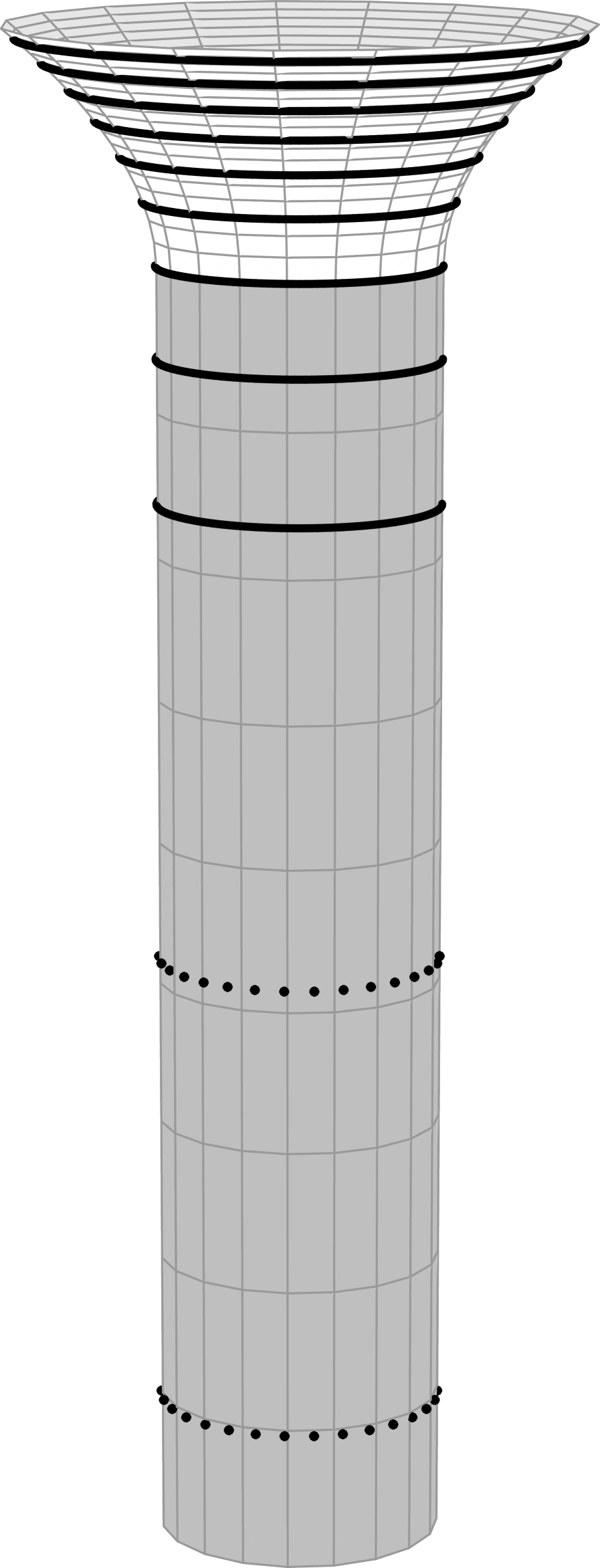
Figure 1: The equatorial submanifold of the optical geometry of the skeleton solution for the stiff matter equation of state ($p=\rho-\rho_{\mathrm{s}}$). The figure represents the star from $r=0.005\,M$ to $r=9.5\,M$. The cylinder is in reality infinitely long in the limit $r\rightarrow 0$. The fat circles represent the surfaces $r=1,2,\ldots,9$ while the dotted curves represent the surfaces $r=0.1$ and $r=0.01$. The shaded region represents the stellar interior.

Figure 2: Plot of $\Sigma$ versus Schwarzschild radial coordinate for some selected values of the central density. The horizontal line at $\Sigma=\frac{1}{2}$ represents the skeleton solution. The remaining curves correspond to the central densities (using clockwise enumeration about the upper left corner of the plot), $\rho_{\mathrm{c}}/\rho_{\mathrm{s}}=1.329,2.09,6.2,30,274$ and $9700$. The most tenuous of the plotted models has $R/M=4$ while the next has $R/M=3$ and is the first ultracompact model in the sequence. The third model has the smallest tenuity in the sequence, $R/M=2.75$. It is a single neck model like the fourth and fifth models. The sixth model is a double neck model represented by the dotted curve. Its inner neck is indicated by the circular disk while the positions of its two bulges are given by the circles. Its outer neck is the Schwarzschild exterior neck at $r=3M$.

To understand the solution space it is necessary to analyze the full 3-dimensional system (5). However, for simplicity, in this communication we restrict attention to the behavior of $\Sigma$. The necks and bulges can then be read off as the zeros of the function $\Sigma-\frac{1}{2}$. Necks and bulges correspond to unstable and stable circular null orbits respectively. The detailed geodesic structure requires a more careful analysis which is beyond the scope of this communication.

The crucial observation comes from the realization that the orbits which correspond to sufficiently compact objects will spiral about the skeleton solution. This happens because the skeleton solution corresponds to a separatrix orbit going from a spiral critical point on the state space boundary at $\Sigma=\frac{1}{2}$, $K=y=\frac{1}{2}$. Since the skeleton solution sits on the surface $\Sigma=\frac{1}{2}$ the number of necks is determined by the number of revolutions in the $\Sigma$-$K$ plane. In the limit of infinite central pressure the number of revolutions grows without limit and hence the number of necks can be arbitrarily large. In figure 2, $\Sigma$ is plotted as a function of the Schwarzschild variable $r$ for some values of the central density including a value which leads to a double neck star.

The null geodesic structure is intimately connected with quasi-normal perturbation modes of the relativistic stellar models [9, 2]. These modes in turn are closely related to gravitational wave scattering. Threfore the appearance of multiple necks is likely to influence the picture of both gravitational pulsation modes and gravitational wave scattering. The examples of multiple neck models we have given in this communication all correspond to unstable stellar objects. Although this would seem to limit the physical applicability of the results, moderately unstable models may in fact have a role to play as intermediate stages in gravitational collapse situations [11]. It is an open problem whether there exist multiple neck models which are both stable and causal. We mention without proof that the stiff fluid equation of state admits a sequence of stable (and of course causal) single neck models but no stable double or higher neck models.

References

- [1] M. Karlovini, K. Rosquist, and L. Samuelsson, Annalen der Physik 9, 149 (2000).
- [2] M. A. Abramowicz et al., Class. Quantum Grav. 14, L189 (1997).
- [3] K. Rosquist, Phys. Rev. D 59, 044022 (1999), (gr-qc/9809033).
- [4] C. Claudel, K. S. Virbhadra, and G. F. R. Ellis, The geometry of photon surfaces, 2000, gr-qc/0005050.
- [5] M. Karlovini, K. Rosquist, and L. Samuelsson, Constructing stellar objects with multiple necks, 2000, (in preparation).
- [6] U. S. Nilsson and C. Uggla, General relativistic static stars: Linear Equations of State, 2000, gr-qc/0002021.
- [7] U. S. Nilsson and C. Uggla, General relativistic static stars: Polytropic Equations of State, 2000, gr-qc/0002022.
- [8] C. Uggla, R. T. Jantzen, and K. Rosquist, Phys. Rev. D 51, 5522 (1995).
- [9] S. Chandrasekhar and V. Ferrari, Proc. Roy. Soc. Lond. A 434, 449 (1991).
- [10] R. C. Tolman, Phys. Rev. 55, 364 (1939).
- [11] D. W. Neilsen and M. W. Choptuik, Class. Quantum Grav. 17, 761 (2000), gr-qc/9812053.