On a General Class of Wormhole Geometries

Abstract

A general class of solutions is obtained which describe a spherically symmetric wormhole system. The presence of arbitrary functions allows one to describe infinitely many wormhole systems of this type. The source of the stress-energy supporting the structure consists of an anisotropic brown dwarf “star” which smoothly joins the vacuum and may possess an arbitrary cosmological constant. It is demonstrated how this set of solutions allows for a non-zero energy density and therefore allows positive stellar mass as well as how violations of energy conditions may be minimized. Unlike examples considered thus far, emphasis here is placed on construction by manipulating the matter field as opposed to the metric. This scheme is generally more physical than the purely geometric method. Finally, explicit examples are constructed including an example which demonstrates how multiple closed universes may be connected by such wormholes. The number of connected universes may be finite or infinite.

PACS numbers: 04.20.Gz, 02.40.Vh, 95.30.Sf

1 Introduction

The study of spacetimes with nontrivial topology is one with an interesting history. One of the earliest, and most famous, wormhole type geometries considered is that of the Einstein-Rosen bridge [1]. This “bridge” connecting two sheets was to represent an elementary particle. That is, particles both charged and uncharged were to be modeled as wormholes. From the work of Einstein and Rosen one also can find a hint to what eventually was to become a central problem in wormhole physics. Energy conditions must generally be violated to support static wormhole geometries.

The wormhole resurfaced later in the study of quantum gravity in the context of the “spacetime foam” [2] [3] in which wormhole type structures permeate throughout spacetime at scales near the Planck length. More recently, there is the meticulous study performed by Morris and Thorne [4] considering a static, spherically symmetric configuration connecting two universes. Since the work by Morris and Thorne, there has been a considerable amount of work on the subject of wormhole physics. For an excellent review the reader is referred to the thorough book by Visser [5] as well as the exhaustive list of references therein. Most interesting is the case of the traversable wormhole which, at the very least, requires tidal forces to be small along time-like world lines as well as the absence of event horizons. These geometries are of interest not only for pedagogical reasons but they serve to shed light on some fundamental issues involving chronology protection [6] and the topology of the universe. Also, many wormhole solutions are in violation of the weak energy condition and there has been much activity in the literature to attempt to minimize such violations (see, for example, [7], [8], [9], [10] and references therein.) There is also the possibility that wormholes have much relevance to studies of black holes. For example, it may be possible that small wormholes may induce large shifts in a black hole’s event horizon or that semiclassical effects near a singularity may cause a wormhole to form avoiding a singularity altogether [11], [12], [13].

For the above reasons, and many others which are hinted at in the literature, it is instructive to study as general a class as possible of such solutions. The aim here is to construct a mathematical model which encompasses the bulk of static, spherically symmetric, wormhole solutions. This is done by studying the profile curve of a generic wormhole structure and postulating a mathematical expression describing this curve. From this ansatz all relevant properties may be calculated. Here we are concerned with making the system as physically relevant, yet as general, as possible. This involves, as much as possible, working with the stress energy tensor when studying the system, as opposed to fully prescribing the geometry as is usually done. We demand that the physical requirements be as reasonable as possible given the situation and study the system from this point of view. Also, the system is not supported by a matter field which permeates all space but possesses a definite matter boundary. At this boundary the solution is smoothly patched to the vacuum with arbitrary cosmological constant. The presence of a cosmological constant is permitted for several reasons. First, astronomical studies of distant supernovae favour the presence of a non-zero cosmological constant [14] [15]. Second, the cosmological constant necessarily violates the strong energy condition and therefore may serve to minimize energy condition violations of the matter field. We make comments where appropriate on how the introduction of the cosmological term affects the behaviour of the matter field. In this paper we find that solutions may be obtained in which the matter field does not violate energy conditions at the throat and with minimal energy condition violation elsewhere. It is possible that a patch to an intermediate layer of matter may eliminate violations altogether.

The paper is organized as follows: Section 2 introduces the Einstein field equations for a general static spherically symmetric system, as well as the differential identities which must be satisfied. This system is then specialized to describe a general wormhole system. Section 3 illustrates the methods used to solve the field equations. The matter field is also introduced and restrictions on its behaviour are analyzed. The singularity and event horizon conditions are studied here in terms of the matter field. The smooth patching of this solution to the exterior Schwarzschild-(anti) de Sitter solution [16] is also covered here along with junction conditions. Specific examples are constructed and energy conditions are studied in section 4. Finally, some concluding remarks are made in section 5.

2 Geometry and Topology

The geometry studied is displayed in figure 1. For the moment we restrict our analysis to the case where there exist two regions, an upper and lower sheet, which are connected by a throat of radius $r=r_{0}$. Neither region need be asymptotically flat and each region may represent a universe which is connected by the wormhole throat. It would not be difficult to modify the calculations here to represent a throat connecting two parts of the same universe. This, for example, may easily be accomplished via topological identification at spatial infinity in the case of an open universe. The closed universe case will be considered as a specific example later.

In the case studied here both the upper and lower universes possess a matter-vacuum boundary at $r=d_{\pm}>r_{0}$ where the $+$ applies to the “upper universe” and the $-$ denotes quantities in the “lower universe”. This boundary represents the junction between the brown dwarf and the vacuum. We use the term brown dwarf to describe the matter system for several reasons. First, the traversability condition precludes the use of a matter system undergoing intense nuclear processes in its interior. A very rough definition of a brown dwarf is a “star” which forms via gravitational collapse but does not ignite nuclear fusion in its core. Second, it is reasonable that if such a system were to form there would be some cut-off point in the stress-energy. Our system here possesses such a boundary (the stellar surface) and therefore the analogy with stellar structure again leads us to the term brown dwarf. It should be noted that $d_{+}$ does not necessarily have to be equal to $d_{-}$ and therefore the brown dwarf “star” may have a different size in each universe.

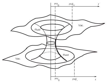
Figure 1: Embedding diagram for the wormhole geometry separating two universes. Circles of constant $r$ represent two-spheres. There is a throat at $r=r_{0}$ and the boundary of the brown dwarf is located at $r=d_{\pm}$ where it is patched smoothly to Schwarzschild-(anti) de Sitter geometry.

We take as our starting point the spherically symmetric line element of the form

$$ds^{2}=-e^{\gamma(r)_{\pm}}\,dt^{2}+e^{\alpha(r)_{\pm}}\,dr^{2}+r^{2}\,d\theta^{2}+r^{2}\sin^{2}(\theta)\,d\phi^{2}$$ (1)

with $\gamma(r)_{\pm}$ and $\alpha(r)_{\pm}$ being functions of the radial coordinate only. The coordinates cover the range

$$-\infty<t<\infty,\;\;0<r_{0}<r<\infty,\;\;0<\theta<\pi,\;\;0\leq\phi<2\pi.$$ (2)

This form will prove especially useful when patching solutions to the vacuum at $r=d_{\pm}$. The condition that there be no horizons implies that $\gamma(r)_{\pm}$ be bounded [17]. Also, we demand that the time-like coordinate, $t$, be smooth across the throat which yields the condition $\gamma(r_{0})_{-}=\gamma(r_{0})_{+}$.

The fundamental equations governing the geometry are the Einstein field equations with cosmological constant

$$R_{\mu\nu}-\frac{1}{2}R\,g_{\mu\nu}+\Lambda\,g_{\mu\nu}=8\pi T_{\mu\nu},$$ (3)

along with the conservation law

$$T^{\mu\nu}_{\;\;\;;\nu}=0.$$ (4)

The spherically symmetric Einstein field equations, in mixed form, yield only three independent equations:

$$G^{0}_{\pm\;0}= \frac{e^{-\alpha(r)_{\pm}}}{r^{2}}\left(1-r\alpha(r)_{\pm,1}\right)-\frac{1}{r^{2}}=8\pi T^{0}_{\pm\;0}-\Lambda$$ (5a)

$$G^{1}_{\pm\;1}= \frac{e^{-\alpha(r)_{\pm}}}{r^{2}}\left(1+r\gamma(r)_{\pm,1}\right)-\frac{1}{r^{2}}=8\pi T^{1}_{\pm\;1}-\Lambda$$ (5b)

$$G^{2}_{\pm\;2}=G^{3}_{\pm\;3}= \frac{e^{-\alpha(r)_{\pm}}}{2}\left(\gamma(r)_{\pm,1,1}+\frac{1}{2}\left(\gamma(r)_{\pm,1}\right)^{2}+\frac{1}{r}\left(\gamma(r)_{\pm}-\alpha(r)_{\pm}\right)_{,1}\right.$$

$$\left.-\frac{1}{2}\alpha(r)_{\pm,1}\gamma(r)_{\pm,1}\right)=8\pi T^{2}_{\pm\;2}-\Lambda=8\pi T^{3}_{\pm\;3}-\Lambda,$$ (5c)

whereas the conservation law yields one non-trivial equation:

$$\frac{r}{2}T^{1}_{\pm 1,1}+\left(1+\frac{r}{4}\gamma(r)_{,1}\right)T^{1}_{\pm 1}-\frac{r}{4}\gamma(r)_{,1}T^{0}_{\pm 0}=T^{2}_{\pm 2}=T^{3}_{\pm 3}.$$ (6)

Note that the cosmological constant, $\Lambda$, is assumed to have the same value in both the $+$ and $-$ region. This is because the cosmological constant is taken to represent the stress-energy of the vacuum and we assume here that both regions, being connected, possess similar vacua. It may be interesting to study situations where, for example, one universe is of de Sitter type and the other of anti-de Sitter type. In this case the de Sitter universe would be a “baby universe” to the anti-de Sitter one.

Equation (5a) may be utilized to give the following:

$$e^{-\alpha(r)_{\pm}} = \frac{8\pi}{r}\int(r^{\prime})^{2}\left(T^{0}_{\pm 0}-\frac{\Lambda}{8\pi}\right)dr^{\prime}+1$$ (7)

$$= \frac{8\pi}{r}\int_{r_{0}}^{r}(r^{\prime})^{2}\left(T^{0}_{\pm 0}-\frac{\Lambda}{8\pi}\right)dr^{\prime}+\frac{c}{r}+1=:1-\frac{b(r)_{\pm}}{r},$$

with $b(r)_{\pm}$ defined as the shape function. If one is considering standard stellar models with plain topology, one must set the constant $c=0$ to avoid a singularity at the origin. Here, however, the origin ($r=0$) is not a part of the manifold (see figure 1) and this constant must be set by the requirement that the throat region be sufficiently smooth, as described next.

Figure 2 shows a cross-section or profile curve of a two dimensional section, $t=\hbox{constant}$, $\theta=\pi/2$, of the wormhole near the throat. The wormhole itself is constructed via the creation of a surface of revolution when one rotates this figure about the $x^{3}$-axis. The surface of revolution may be parameterized as follows

$$x(r,\phi):=\left(x^{1}(r,\phi),\,x^{2}(r,\phi),\,x^{3}(r,\phi)\right)=\left(r\cos(\phi),\,r\sin(\phi),\,P(r)\right),$$ (8)

where $r=\sqrt{\left(x^{1}\right)^{2}+\left(x^{2}\right)^{2}}$ and $\phi$ is shown in figure 2. Therefore, the induced metric on the surface is given by

$$d\sigma^{2}=\left[1+P_{,1}(r)^{2}\right]\,dr^{2}+r^{2}\,d\phi^{2},$$ (9)

where commas denote ordinary derivatives. Note that the corresponding four-dimensional spacetime metric, (1), may now be written as:

$$ds^{2}=-e^{\gamma(r)}\,dt^{2}+\left[1+P_{,1}(r)^{2}\right]\,dr^{2}+r^{2}\,d\theta^{2}+r^{2}\sin^{2}(\theta)\,d\phi^{2}.$$ (10)

The shape function, $b(r)$, may now be specified in terms of the embedding function, $P(r)$, which will be discussed shortly.

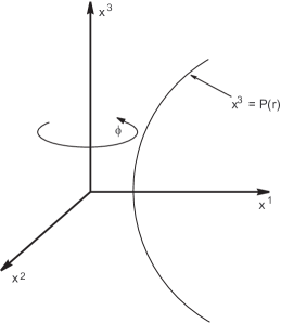
Figure 2: A cross section of the wormhole profile curve near the throat region. The wormhole is generated by rotating the curve about the $x^{3}$-axis.

To set the constant, $c$, in (7) note that from the profile curve in figure 2 the derivative $P_{,1}(r)$ tends to infinity as one approaches $r_{0}$. This condition translates, via (10), to $1-b(r)_{\pm}/r$ vanishing at $r=r_{0}$. Therefore the constant $c$ must be equal to $-r_{0}$. This condition is equivalent to that in [4] and reflects the fact that at the throat a finite change in coordinate distance, $\Delta r$, corresponds to an infinite change in proper radial distance, $\Delta l$. That is,

$$\lim_{r\rightarrow r_{0}}(\Delta l)=\lim_{r\rightarrow r_{0}}\frac{\Delta r}{\sqrt{1-\frac{b(r)_{\pm}}{r}}}\rightarrow\infty.$$ (11)

A final condition for smooth patching is the continuity of the second fundamental form [18]. For the moment we assume that the joining of the upper and lower universes may be performed. It will be shown, in section 3, that the second fundamental form is indeed continuous however; a few more properties of the system need to be studied in order to demonstrate this.

We are now in a position to analyze the geometry. For now we limit the analysis to the top half of the profile curve (the “+” region) since the bottom half is easily obtained once we have the top half. From the profile curve in figure 2 it may be seen that a function is needed with the following properties:

• The derivative, $P_{,1}(r)$, must be infinite at the throat and finite elsewhere.

• The derivative, $P_{,1}(r)$, must be positive at least near the throat.

• The function $P(r)$ must possess a negative second derivative at least near the throat region.

• Since there will be a cut-off at $r=d$, where the solution is joined to vacuum (Schwarzschild-(anti) de Sitter), no specification needs to be made as $r$ tends to infinity.

These restrictions are purely geometric in nature. We show below that reasonable physics will demand further restrictions. From these properties a general function is assumed of the form:

$$P(r) =A\left(r-r_{0}\right)^{\epsilon}\exp\left[-h(r)\right],$$ (12a)

$$P_{,1}(r) =P(r)\left[\epsilon\left(r-r_{0}\right)^{-1}-h_{,1}(r)\right],$$ (12b)

$$P(r)_{,1,1} =P(r)\left\{\left[\epsilon\left(r-r_{0}\right)^{-1}-h_{,1}(r)\right]^{2}-h(r)_{,1,1}-\epsilon\left(r-r_{0}\right)^{-2}\right\}.$$ (12c)

Here $h(r)$ is any non-negative (at least twice differentiable) function with non-negative first derivative. Moreover, $\epsilon$ is a constant bounded as follows: $0<\epsilon<\frac{1}{2}$. The reason for this restriction will be made clear later. $A$ is a positive constant which is required so that quantities possess correct units (the unit of $A$ is $\hbox{length}^{1-\epsilon}$.) One may enforce conditions on $h(r)$ by writing it in terms of a slack function as

$$h_{,1}(r) = \hbox{e}^{q(r)},$$

$$h(r) = \int_{r_{0}}^{r}\hbox{e}^{q(r^{\prime})}\,dr^{\prime}+z_{0},$$

with $z_{0}$ a constant and $q(r)$ an arbitrary differentiable function.

The shape function, $b(r)$, is given by (7) and (10)

$$b(r)= r\frac{P_{,1}(r)^{2}}{1+P_{,1}(r)^{2}},$$ (13a)

$$b(r)_{,1}= \frac{P_{,1}(r)}{1+P_{,1}(r)^{2}}\left[P_{,1}(r)+\frac{2rP(r)_{,1,1}}{1+P_{,1}(r)^{2}}\right].$$ (13b)

The bottom universe may be obtained via the profile curve by demanding that $A$ be some negative constant. The first derivative will then be negative near the throat and the second derivative positive. The function $h(r)$ may be different in the lower universe than in the upper and this will not spoil smoothness at the throat as long as $h_{+}(r_{0})=h_{-}(r_{0})$ and $h_{+,1}(r_{0})=h_{-,1}(r_{0})$.

To show that the system is indeed a wormhole with a smooth patching at $r_{0}$, it is useful to show that the system may be described by a single coordinate chart across the throat. Consider the profile curve in the $x^{1}x^{3}$-plane of figure 2. The upper half of this curve may be described by

$$x^{1}= X_{+}^{1}(r_{+}):=r_{+},$$ (14a)

$$x^{3}= X_{+}^{3}(r_{+}):=P_{+}(r_{+}),$$ (14b)

with the $+$ subscripts indicating the upper universe with $r_{+}>r_{0}$. We denote the inverse of $P_{+}(r_{+})$ from (14b) as $r_{+}=P_{+}^{\sharp}(x^{3})$ ($\sharp$ superscripts will be used to indicate inverse mappings). Also, the lower half of the curve is given by

$$x^{1}= X_{-}^{1}(r_{-}):=r_{-},$$ (15a)

$$x^{3}= X_{-}^{3}(r_{-}):=P_{-}(r_{-}),$$ (15b)

and again $r_{-}>r_{0}$ with $r_{-}=P_{-}^{\sharp}(x^{3})$. At the moment we have two charts in two universes and we may construct two metrics from these (the “+” and “-” metrics from above). The unifying chart, which includes both universes near the throat as well as the boundary, $r_{0}$, is given by studying the profile curve as a function of $x^{3}$. In other words, we rotate the $x^{1}x^{3}$-plane about the $x^{2}$-axis of figure 2 by $\pi/2$ and study the profile curve parameterized by the coordinate $x^{3}$. By equation (12a), $x^{3}$ belongs to an interval containing $x^{3}=0$ which corresponds to the throat of the wormhole ($r_{0}$ corresponds to $P^{\sharp}(0)$). With this parameterization, $P^{\sharp}(0)=r_{0}$ exists as well as $\lim_{x^{3}\rightarrow 0_{+}}P^{\sharp}(x^{3})=\lim_{x^{3}\rightarrow 0_{-}}P^{\sharp}(x^{3})$ and therefore $P^{\sharp}$ is continuous. The functions $P^{\sharp}_{+}(x^{3})$ and $P^{\sharp}_{-}(x^{3})$ are simply obtained by the restrictions of $P^{\sharp}(x^{3})$ in $x^{3}>0$ and $x^{3}<0$ respectively. The resulting curve is parameterized as:

$$x^{1}= X^{\sharp\;1}(x^{3})=P^{\sharp}(x^{3}),$$ (16a)

$$x^{3}= X^{\sharp\;3}(x^{3}):=x^{3}.$$ (16b)

With this “universal” chart the spacetime metric near the throat may be written as

$$ds^{2}=-e^{\gamma^{\prime}(x^{3})}\,dt^{2}+\left[1+P^{\sharp}_{,x^{3}}(x^{3})^{2}\right]\,(dx^{3})^{2}+P^{\sharp}(x^{3})^{2}\,d\theta^{2}+P^{\sharp}(x^{3})^{2}\sin^{2}\theta\,d\phi^{2}.$$ (17)

This single metric is therefore sufficient to describe both parts of the wormhole system across the throat.

In the coordinate chart used thorughout most of this paper, (10), the manifold must be at least piece-wise $C^{3}$ smooth to have a well behaved Einstein tensor with contracted Bianchi identity. At the throat junction we will later show that a minimum of $C^{1}$ is admitted although there is no reason why a higher, perhaps more physical, class may not be admitted. It may be argued that the chart given by (17) is better suited for studies across the throat. In that case the embedding function, $P^{\sharp}(x^{3})$, may be chosen of arbitrary differentiability class (ideally minimum $C^{4}$ to give a $C^{3}$ manifold) and no piece-wise considerations need be addressed at the throat. The coordinate transformations from one chart to the other, however, may turn out to be formidable. The above discussion refers to the differentiability of the metric. Since the metric depends on the derivative of the profile curve, a $C^{n}$ manifold should possess a $C^{n+1}$ profile curve.

3 Wormhole Structure

In this section the field equations are utilized to construct the wormhole structure. There are a number of ways to proceed and each method has its particular advantages and disadvantages. One method is a purely geometric method or g-method [19]. In this method one is free to specify the metric components, $\gamma(r)$ and $b(r)$, to acquire the desired geometry. One then completely determines the supporting stress-energy tensor from the geometry via the field equations. This is the method of [4]. One may, for example, wish that $\gamma(r)$ be bounded to eliminate horizons. As a simple example, such a function may be expressed in terms of a sum of an even and an odd bounded function as:

$$\gamma(r)=c_{1}\tanh(\varphi(r))+c_{2}\,\,\hbox{sech}(\psi(r)),$$ (18)

which is bounded as

$$|\gamma(r)|\leq|c_{1}|+|c_{2}|.$$ (19)

Here $\varphi(r)$ and $\psi(r)$ are arbitrary. This method possesses the advantage that any reasonable geometry allowed by general relativity may be constructed. The disadvantage, however, is that one may be left with a stress-energy tensor which is physically unreasonable.

A second method is the T-method [19]. Here one prescribes properties of a desired matter field and from this constructs a stress-energy tensor. The field equations are then solved for the metric which governs the geometry. This is generally a preferred method as one may prescribe physically reasonable matter and study the resulting gravitational field. The disadvantage, of course, is that there is very little control over the geometry. If we have a particular geometry in mind, there is no guarantee that an a priori prescribed stress-energy tensor will generate the desired gravitational field. Therefore, for the purposes of wormhole analysis, this method is not useful.

A third method, and one which most of the analysis here is based on, is a mixed method [20]. This method may be implemented in two ways:

• Prescribe some desirable physical properties to $T^{\>0}_{\pm 0}$ and $T^{\>1}_{\pm 1}$. For instance, for physically reasonable matter one may wish the first to be negative and the latter non-negative. Otherwise, $T^{\>1}_{\pm 1}$ may be freely set. $T^{\>0}_{\pm 0}$ may be obtained via the shape function, $b(r)_{\pm}$, using (5a). The physical properties demanded above must be utilized to constrain the shape function. The transverse pressures $T^{\>2}_{\pm 2}=T^{\>3}_{\pm 3}$ are defined via (6).

• Again obtain $T^{\>0}_{\pm 0}$ from the shape function as above and prescribe an equation of state relating $T^{\>1}_{\pm 1}$ to $T^{\>0}_{\pm 0}$. Again the transverse pressures are obtained from (6).

All equations will then be satisfied. The advantage of this method is that one may employ some reasonable physical assumptions on the matter fields, yet not give up all control over the geometry. The major disadvantage is that, since $g_{00}$ is not set, certain desirable properties of the manifold, such as the absence of horizons and curvature singularities, are not guaranteed. These problems will be addressed below.

The matter field may, for example, be that of an anisotropic fluid whose stress-energy tensor is given by

$$T_{\mu\nu}=\left(\rho+p_{\perp}\right)u_{\mu}u_{\nu}+p_{\perp}\,g_{\mu\nu}+\left(p_{\shortparallel}-p_{\perp}\right)s_{\mu}s_{\nu}$$ (20)

with

$$u^{\mu}u_{\mu}= -1,$$ (21a)

$$s^{\mu}s_{\mu}= 1,$$ (21b)

$$u^{\mu}s_{\mu}= 0.$$ (21c)

Here, in the static case, the eigenvalues of $T^{\mu}_{\nu}$ are $T^{0}_{\;0}=-\rho$, $T^{1}_{\;1}=p_{\shortparallel}$ and $T^{2}_{\;2}=T^{3}_{\;3}=p_{\perp}$ which are a measure of the (negative) energy density, radial pressure and transverse pressure, respectively. This matter model fits our prescription for several reasons. First, the construction of static, spherically symmetric wormholes requires a stress-energy tensor which admits four real eigenvalues. Two of these eigenvalues coincide by demanding spherical symmetry ($T^{2}_{\>2}$ and $T^{3}_{\>3}$). Second, utilizing both the g and mixed methods will most likely result in a system possessing three distinct eigenvalues. Furthermore, it is known that these eigenvalues must, at least in some vicinity, violate energy conditions [4]. It has been shown [21] that the anisotropic fluid, when undergoing gravitational collapse, may form many states of “exotic” (energy condition violating) matter. Finally, a wormhole system as described in this paper would most likely form via gravitational collapse, as with normal stars. The anisotropic fluid therefore represents a matter field which is a reasonable extension of certain standard stellar models involving a perfect fluid [22].

The metric function , $\gamma_{\pm}(r)$, is given by (5b) and its integral:

$$\gamma(r)_{\pm,1}= \left(8\pi T^{\>1}_{\pm 1}(r)-\Lambda+\frac{1}{r^{2}}\right)\frac{r}{1-\frac{b_{\pm}(r)}{r}}-\frac{1}{r},$$ (22a)

$$\gamma(r)_{\pm}= \int_{r_{0}}^{r}\left(8\pi T^{\>1}_{\pm 1}(r^{\prime})-\Lambda+\frac{1}{(r^{\prime})^{2}}\right)\frac{r^{\prime}\,dr^{\prime}}{1-\frac{b_{\pm}(r^{\prime})}{r^{\prime}}}-\ln(r)+K_{\pm},$$ (22b)

with $K_{\pm}$ a constant. Continuity of $\gamma(r)_{\pm}$ at the throat requires that $K_{+}=K_{-}$; $\alpha(r)_{\pm}$ is given by equation (7):

$$\alpha(r)_{\pm}= -\ln\left[1-\frac{r_{0}}{r}+\frac{8\pi}{r}\int_{r_{0}}^{r}(r^{\prime})^{2}\left(T^{0}_{\pm 0}-\frac{\Lambda}{8\pi}\right)\,dr^{\prime}\right]$$

$$= -\ln\left(1-\frac{b_{\pm}(r)}{r}\right),$$ (23a)

$$\alpha(r)_{\pm,1}= \frac{1}{r\left(1-\frac{b_{\pm}(r)}{r}\right)}\left(b(r)_{\pm,1}-\frac{b(r)_{\pm}}{r}\right).$$ (23b)

Another useful equation, which will be utilized later, is obtained by subtracting (5a) from (5b)

$$8\pi e^{\alpha(r)_{\pm}}r\left(T^{1}_{\pm 1}-T^{0}_{\pm 0}\right)=\left(\gamma(r)_{\pm}+\alpha(r)_{\pm}\right)_{,1}\;\;.$$ (24)

Having expressions for the metric functions and their derivatives, we now turn to the matter field. This analysis will allow us to determine all properties which the general embedding function need to satisfy and will therefore provide a general class of metrics describing such wormholes.

The Einstein equation (5a) may be written in terms of the shape function yielding:

$$-\frac{1}{r^{2}}b(r)_{,1}=8\pi T^{\>0}_{\pm 0}-\Lambda.$$ (25)

We assume here that, at least in the vicinity of the throat where the cosmological constant is negligible compared to the matter energy density, the net energy density is positive. From (25) it is seen that this requires that $b(r)_{,1}>0$ near the throat. Recall from the properties of the profile curve (figure 2), $P(r)$ must possess positive first derivative and negative second derivative near the throat. From (13b) it may be seen that if the second term in the expression dominates, $b(r)_{,1}$ will be negative which is not desirable. Therefore (13b) must be analyzed with some care in the vicinity of the throat.

To study the properties of (25) near the throat, we define a parameter $\delta:=(r-r_{0})$. Analysis of $b(r)_{,1}$ then shows that

$$b(r)_{,1}\approx 1-\mathcal{O}(\delta^{1-2\epsilon})+\ldots$$ (26)

from which it may be seen that $\epsilon$ must be restricted to the interval $0<\epsilon<\frac{1}{2}$, as mentioned earlier. Note that $\epsilon=\frac{1}{2}$ is allowed, although a negative energy density as observed by static observers is the price one pays for this case. Even for the values of $\epsilon$ stated above $b(r)_{,1}$ eventually becomes negative at some radius, $r=r_{\pm}^{*}$ say, as is evident from (13b). One could, if one insists on a positive value of $b(r)_{,1}$ everywhere, place the stellar boundary at $d_{\pm}<r_{\pm}^{*}$. Note that since the model admits an arbitrary cosmological constant, we could allow $b(d_{\pm})_{,1}<0$ and still claim a positive $\rho$ for the matter field if $\Lambda<0$.

The equation (26) with the above restriction on $\epsilon$ yields the best possible scenario as far as the energy density is concerned. That is, a value of $b(r)_{\pm,1}$ greater that unity cannot be achieved at the throat. This situation is quite favourable with respect to the energy conditions (to be discussed section 4) as the null, weak and dominant energy conditions each require positivity of energy density.

3.1 Horizons and Singularities

As mentioned earlier, the method utilized here, although giving some control over the matter fields, does not guarantee the absence of event horizons nor singularities. In this section we address both of these issues. The notation $\tau(r):=8\pi T^{1}_{\;1}-\Lambda$ is used throughout this section.

In the coordinate system of (1) an event horizon will exist wherever $g_{00}$ vanishes. In other words, the function $\gamma_{\pm}(r)$ must be everywhere finite. Using (22a) and (22b) it may be seen that, to ensure that $\gamma(r)_{\pm}$ remain finite near the throat, $(\tau(r)+1/r^{2})$ must vanish at least as fast as $(r-b(r)_{\pm})$ in the limit $r\rightarrow r_{0}$.

From (13a) it may be shown that near the throat

$$\left(b(r)-r\right)\propto\left(r-r_{0}\right)^{2(1-\epsilon)};$$ (27)

therefore the numerator of the first term in (22a) must possess behaviour near the throat of the form $(r-r_{0})^{\eta}$ with $\eta\geq 2(1-\epsilon)$ and

$$\tau(r_{0})=-1/r_{0}^{2},$$ (28)

Although we may possess everywhere non-negative energy density, (28) shows that a negative pressure or tension is required at the throat to support the wormhole. The fluid pressure may still be positive if the cosmological constant is positive and dominates the fluid pressure at the throat.

The equation (22b) may most easily be made well behaved for any $\epsilon$ allowed by the model by demanding that the first-order term in the expansion of $\tau(r)+1/r^{2}$ about $r_{0}$ vanish. Also, the appropriate limit $\tau(r_{0})=-1/r_{0}^{2}$ must be enforced so that the zeroth-order term vanish as well. With little loss of generality we may write $\tau(r)$ as

$$\tau(r) = -\frac{1}{r^{2}}\cos\left[\frac{(r-r_{0})}{(d+\alpha-r_{0})}\frac{m\pi}{2}\right]\cosh\left[(r-r_{0})^{s}\xi(r)\right]$$ (29)

$$+ \kappa(r-r_{0})^{q}(r-d)^{w}\exp\left(\zeta(r)\right)$$

with $m$ an odd integer, $q\geq 2,w>0$ positive integers and $\xi(r)$ and $\zeta(r)$ arbitrary functions save for the restriction that they possesses well behaved derivatives in the regime $r_{0}\leq r\leq d$; $\alpha$ is a small constant set by the requirement that at $r=d_{\pm}$ the above expression is equal to $-\Lambda$. The second term, proportional to the constant $\kappa$, is not strictly required, though it is useful in making $\tau(r)$ positive throughout most of the stellar region (see section 4). An analysis of the matter field in the context of the energy conditions may also be found in section 4.

Having eliminated the possibility of event horizons, it is now necessary to analyze the manifold for singularities. Singular manifold structure is most easily studied by constructing the Riemann tensor in an orthonormal frame. We use notation such that indices surrounded by parentheses denote quantities in the orthonormal frame. In this frame the Riemann tensor possesses the following components as well as those related by symmetry [4]:

$$R_{(trtr)\pm}= \frac{1}{2}\left(1-\frac{b_{\pm}(r)}{r}\right)\left[\gamma(r)_{\pm,1,1}+\frac{1}{2}(\gamma(r)_{\pm,1})^{2}\right.$$

$$-\left.\frac{1}{2}\gamma(r)_{\pm,1}\frac{b(r)_{\pm,1}-\frac{b_{\pm}(r)}{r}}{r-b_{\pm}(r)}\right]\;\;,$$ (30a)

$$R_{(t\theta t\theta)\pm}= \frac{1}{2r}\gamma(r)_{\pm,1}\left(1-\frac{b_{\pm}(r)}{r}\right)=R_{(t\phi t\phi)\pm}\;\;,$$ (30b)

$$R_{(r\theta r\theta)\pm}= \frac{1}{2r^{2}}\left[b(r)_{\pm,1}-\frac{b_{\pm}(r)}{r}\right]=R_{(r\phi r\phi)\pm}\;\;,$$ (30c)

$$R_{(\theta\phi\theta\phi)\pm}= \frac{b_{\pm}(r)}{r^{3}}\;\;.$$ (30d)

Recall that, utilizing our ansatz (12a) with (13a) and (13b), $b(r_{0})=r_{0}$ and $b(r_{0})_{,1}=1$. Therefore all components of the Riemann tensor, with the possible exception of (30a), are finite at the throat. The only other problematic spot is $r=0$, which is not a part of the manifold and therefore causes no concern for our analysis. The previous restrictions on $\tau(r)_{\pm}$ ensure that $\gamma(r)_{\pm}$ and its derivatives are finite away from the throat. No quantity grows without bound as we move away from the throat.

To study (30a) more carefully, it is useful to write it in terms of $T^{\>1}_{\pm 1}$ using (22a) as (dropping the $\pm$ subscript for now)

$$R_{(trtr)} = \frac{1}{4r^{3}\left(r-b(r)\right)}\left[\tau(r)^{2}r^{6}+2r^{4}\tau(r)_{,1}\left(r-b(r)\right)\right.$$ (31)

$$+ r^{3}\tau(r)\left(2r-b(r)+rb(r)_{,1}\right)-4rb(r)+2r^{2}b(r)_{,1}$$

$$+ \left.4b(r)^{2}-b(r)b(r)_{,1}r\right].$$

Notice that for non-singular behaviour, the term in square brackets must vanish at least as fast as the denominator as $r\rightarrow r_{0}$. Recall that the denominator’s behaviour is as in (27) and therefore the numerator must possess similar or stronger vanishing properties here. An exhaustive calculation using (29) reveals that the numerator does indeed vanish at least as fast as the denominator near the throat and therefore all curvature tensor components are finite, eliminating any singularities. It is interesting to note that, by demanding that $\gamma(r)_{\pm,1}$ be finite everywhere (the horizon condition), we also impose the final condition which ensures finiteness on all orthonormal Riemann tensor components. In other words, naked singularities are not supported.

We now return to the consideration regarding the continuity of the second fundamental form at the throat. The second form is most easily calculated in the coordinate frame as the covariant derivative

$$K_{\mu\nu}=\frac{1}{2}\left(\hat{n}_{\mu;\nu}+\hat{n}_{\nu;\mu}\right),$$ (32)

where $\hat{n}_{\mu}$ represents an outward pointing radial unit vector which, using (10), is given by:

$$\hat{n}_{\mu}=\sqrt{1+P_{,1}(r)^{2}}\;\;\delta^{(r)}_{\;\mu}$$ (33)

(the $\pm$ subscripts have been dropped here). From (32) the following components are calculated for the second fundamental form:

$$K_{tt}= -\frac{1}{2\sqrt{1+P_{,1}(r)^{2}}}\hbox{e}^{\gamma(r)}\gamma_{,1}(r)\;,$$ (34a)

$$K_{\theta\theta}= \frac{r}{\sqrt{1+P_{,1}(r)^{2}}}\;,$$ (34b)

$$K_{\phi\phi}= \frac{r\sin^{2}\theta}{\sqrt{1+P_{,1}(r)^{2}}}\;.$$ (34c)

(34b) and (34c) are certainly continuous at the throat since, from (12b) they both vanish as one approaches $r=r_{0}$ from either the “+” region or the “-” region. $K_{tt}$ will be studied with some care. Recall that the condition ensuring the absence of horizons is given by demanding that (22a) be everywhere finite. This condition therefore requires that $\tau(r_{0}):=8\pi T^{1}_{\;1}(r)-\Lambda=-1/r_{0}$ and this result is, of course, independent of the region in which one is approaching $r_{0}$. This condition, along with the fact that $b_{+}(r_{0})=b_{-}(r_{0})=r_{0}$ dictates, via (22a), that $\gamma_{,1}(r)$ be continuous at the throat. Also, continuity of the metric requires that $\hbox{e}^{\gamma(r_{0})_{+}}=\hbox{e}^{\gamma(r_{0})_{-}}$ and therefore $K_{tt}$ must also be continuous at the throat. All required junction conditions at the throat have therefore been met (namely: continuity of the metric, $T^{1}_{\;1}(r)$, and the second fundamental form as well as condition (11) along with visual proof from figure 4b to be discussed in section 4).

If one is considering a traversable type wormhole then a further restriction on Riemann components is generally desired. Namely, the magnitude of these components must be small in the sense that tidal acceleration, given by:

$$\Delta a^{\mu}=R^{\mu}_{\;\alpha\beta\gamma}V^{\alpha}V^{\beta}\Delta\xi^{\gamma}$$ (35)

be sufficiently small to allow travel through the throat. Here $\Delta\xi^{\gamma}$ is a separation vector joining two parts of the traveling body. The condition that (35) be small places constraints on the magnitude of the orthonormal Riemann tensor components as well as on the velocity at which the wormhole may safely be traversed [3], [5]. At the throat, it is possible to make all components of (30a)-(30d) small or vanish due to the fact that $b(r_{0})=r_{0}$ and $b(r_{0})_{,1}=1$, with possible exception of (30d) which is equal to $1/r_{0}^{3}$. For purely radial motion (35) dictates that this component plays no part in the tidal acceleration and therefore presents no constraint on the wormhole size [3], [5]. Away from the throat there is the potential to make the relevant components at least reasonably small by the choice of matter field via (22a) and (31). Note that the “smallness” of the Riemann components is not a requirement of the wormhole system. It is simply a measure of the ease at which one may be traversed.

3.2 The Stellar Boundary

Having identified conditions in the interior we now turn attention to the boundary of the star at $r=d_{\pm}$. Here the solution must smoothly tend to the vacuum Schwarzschild-(anti) de Sitter metric:

$$ds^{2}= - \left(1-\frac{2M_{0\pm}}{r}-\frac{1}{3}\Lambda\,r^{2}\right)d\tilde{t}^{2}+\frac{dr^{2}}{\left(1-\frac{2M_{0\pm}}{r}-\frac{1}{3}\Lambda\,r^{2}\right)}$$ (36)

$$+ r^{2}\,d\theta^{2}+r^{2}\sin^{2}(\theta)\,d\phi^{2}$$

where the tilde on the time coordinate will be later made clear. Note that the “mass” of the star in one universe need not necessarily be the same as in the other. The junction condition employed at this surface will be that of Synge [19]

$$\left.T^{\mu}_{\pm\nu}n^{\nu}\right|_{r=d_{\pm}}=0$$ (37)

with $n^{\nu}$ an outward pointing radial normal vector. This condition essentially states that there may be no flux of stress-energy off the surface of the star which, of course, is a reasonable requirement when patching to a vacuum solution as will be done next. For the class of metrics considered here, continuity of the metric at the boundary also ensures continuity of the extrinsic curvature.

It is now necessary to check conditions at the boundary $r=d_{\pm}$ where the interior solution must match the vacuum solution given by (36). Here, from (7) we get

$$e^{\alpha(d_{\pm})}=\left[1-\frac{2M_{\pm}}{d_{\pm}}+\frac{\Lambda}{3}\frac{r_{0}^{3}}{d_{\pm}}-\frac{r_{0}}{d_{\pm}}-\frac{\Lambda}{3}d_{\pm}^{2}\right]^{-1},$$ (38)

where $M_{\pm}$ corresponds to the fluid mass,

$$M_{\pm}=-4\pi\int_{r_{0}}^{d_{\pm}}(r^{\prime})^{2}T^{0}_{\pm\;0}\,dr^{\prime}.$$ (39)

The function (38) matches smoothly to the Schwarzschild-(anti) de Sitter metric (36) with an “effective mass”

$$M_{0\pm}=M_{\pm}-\frac{\Lambda}{6}r_{0}^{3}+\frac{r_{0}}{2}.$$ (40)

The equation for $\gamma_{\pm}$ is more complicated:

$$e^{\gamma(d_{\pm})} = \left(1-\frac{2M_{0\pm}}{d_{\pm}}-\frac{\Lambda}{3}d^{2}_{\pm}\right)$$ (41)

$$\times \exp\left\{8\pi\int_{r_{0}}^{d_{\pm}}\frac{(r^{\prime})^{2}(p_{\pm\shortparallel}+\rho_{\pm})\;dr^{\prime}}{\left[r^{\prime}-8\pi\int_{r_{0}}^{r^{\prime}}(r^{*})^{2}(\rho_{\pm}+\frac{\Lambda}{8\pi})\,dr^{*}-r_{0}\right]+K}\right\}$$

$$=: \left(1-\frac{2M_{0\pm}}{d_{\pm}}-\frac{\Lambda}{3}d^{2}_{\pm}\right)e^{2\chi_{\pm}}.$$

Here (24) has been used. We now perform the following coordinate change

$$\tilde{t}=e^{\chi}t$$ (42)

so that

$$\left(d\tilde{t}\right)^{2}=e^{2\chi}dt^{2}$$ (43)

and thus the interior solution has been matched to (36).

4 Examples

Having developed the formalism for constructing such wormholes it is instructive to demonstrate how the scheme works via specific examples. Again the $\pm$ subscript is neglected unless needed for clarity.

A simple, yet instructive example is one with the following parameters:

$$h(r)\propto \;\;r^{2}\>,$$

$$\xi(r)\propto \;\;r^{3}\>,$$

$$m= \;\;3,$$

$$s= \;\;1,$$

$$\Lambda\sim \;\;\hbox{small and positive},$$

$$\kappa\sim \;\;\hbox{large and positive},$$

$$\zeta(r) \;\;\hbox{a constant}.$$

The rotated profile curve for this system is shown in figure 3a. Figure 3b displays the shape function and 3c its derivative. Note that the total mass (as measured by $b(r)$) and the energy density ($b(r)_{,1}$) are positive in the vicinity of the throat. Since the Einstein equations permit discontinuities in the energy density, there is no reason to place the stellar boundary near the point where $b(r)_{,1}$ vanishes although for this example we do so. The radial pressure, $p_{\shortparallel}=\left(\tau(r)+\Lambda\right)/8\pi$, is plotted in figure 3d. Note that with the addition of the large $\kappa$ term this term is positive throughout most of the region. Finally, figure 3e shows a plot of the transverse pressure. As with the radial pressure, this quantity is positive throughout most of the stellar bulk.

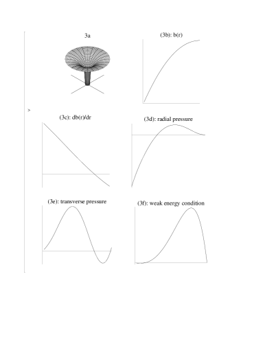
Figure 3: A sample wormhole system. a) shows a rotated profile curve of the “+” universe. b) is a plot of the effective mass of the star, c) a plot of the effective energy density, $b(r)_{,1}$, d) the parallel pressure e) the transverse pressure and f) the weak energy condition. Note that $\rho$ is non-negative. Moreover, throughout most of the stellar bulk $p_{\shortparallel}$ and $p_{\perp}$ are positive.

4.1 Energy Conditions

Here we discuss energy conditions both in general and with respect to the above example. From an expansion of (25) near the throat we find that

$$8\pi\rho \approx \frac{1}{r_{0}^{2}}-\Lambda+\frac{2}{A^{2}\epsilon r_{0}}\hbox{e}^{2h(r_{0})}\left(1-\frac{1}{\epsilon}\right)\left(r-r_{0}\right)^{1-2\epsilon}-\frac{2}{r_{0}^{3}}\left(r-r_{0}\right)$$ (45)

$$- \frac{1}{A^{2}\epsilon^{2}r_{0}^{2}}\hbox{e}^{2h(r_{0})}\left(r-r_{0}\right)^{2(1-\epsilon)}.$$

A similar analysis on the radial pressure yields via (29):

$$8\pi p_{\shortparallel}\approx-\frac{1}{r_{0}^{2}}+\Lambda+\frac{2}{r_{0}^{3}}(r-r_{0})+\mathcal{O}(r-r_{0})^{2}.$$ (46)

Finally, the transverse pressure (6)

$$8\pi p_{\perp}(r_{0})=8\pi\frac{r_{0}}{2}p_{\shortparallel,1}|_{r=r_{0}}-\frac{1}{r_{0}^{2}}+\Lambda=\Lambda.$$ (47)

Exactly at the throat, energy conditions are respected as $\rho$ is positive unless the cosmological constant is large (a possibility ruled out by experiment) and $\rho(r_{0})+p_{\shortparallel}(r_{0})=0$ as well as $\rho(r_{0})+p_{\perp}(r_{0})>0$. As we move away from the throat notice that, in the expression $\rho+p_{\shortparallel}$, the third and fifth terms of (45) survive. Both of these terms yield a negative contribution and therefore energy conditions are violated slightly away from the throat. It is possible to cut-off the solution at some radius near $r_{0}$ and patch to an intermediate layer of material which respects energy conditions. This intermediatelayer may then be patched to the Schwarzschild-(anti) de Sitter vacuum and thus there will be little or no energy condition violation. Notice from figure 3 that averaged energy conditions (energy conditions integrated over the stellar bulk) are certainly satisfied as most of the stellar bulk is “well behaved” in the context of energy conditions. Also interesting is that, at the throat, the matter is still exotic in the sense that the magnitude of the pressure is of the same order of magnitude as the energy density. A positive cosmological constant, if present, would minimize the amount of material needed at the throat although the cosmological constant would most likely be quite small when compared to $1/r_{0}^{2}$ and therefore would not necessarily eliminate this exotic behaviour.

The weak energy condition may also most easily be studied by forming the quantity [4], [8]

$$\varepsilon:=\frac{(p_{\shortparallel}+\rho)}{|\rho|}.$$ (48)

This quantity should be positive for any matter respecting the weak energy condition. We plot this quantity for the example above in figure 3f. This figure shows that throughout the stellar bulk, with the exception of a small region near (but not at) the throat, the weak energy condition is satisfied. The violation, however, is very small. This agrees with the perturbative analysis above, as well as with [23], where it si shown that the energy violations can be confined to an arbitrarily small region around the throat provided that $b_{1}(r)$ is close to unity. As pointed out in much of the literature on energy conditions, this violation does not conflict with experimental results as the weak energy violating Casimir effect has been verified experimentally [24].

Another interesting example, which we will briefly consider, is that where the wormhole connects not just two universes but any number of universes. An in-depth analysis of this situation will not be made and this example simply serves to illustrate that a minor extension to the above techniques is all that is required for such a system.

The profile curve of the “top half” of a single closed universe is shown in figure 4a. The bottom half of the universe may be generated by reflection via $P(r)\rightarrow-P(r)$. We use as an example of such a profile curve the following function:

$$P(r)=\frac{1}{k}\cos^{-1}\left[\frac{(r-B)}{R}\right],$$ (49)

where $k$, $R$ and $B$ are constants (with $B>R$) related to the size of the universe and to the size of the throat via $d=B+R$ and $r_{0}=B-R<<B+R$. This profile, along with its reflection about the $r$-axis serves to generate the closed universe. Note that this universe may be joined at its throats to other (potentially infinite number of) closed universes or to an open universe at each end of the closed universe chain. In this latter case the closed system represents a set of “baby universes” to the open ones. It should also be possible to terminate the chain not with open universes but instead a closed universe with only one throat. Note that continuity of the metric must be respected at each coordinate chart junction in order to have a smooth patching. A representative system of three closed universes with similar radii is shown in figure 4b.

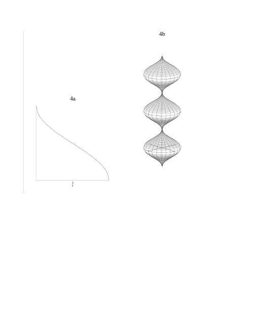
Figure 4: a) The profile curve for the upper section of a single universe. b) A chain of three closed universes connected by wormholes.

Again we utilize the mixed method of solving the Einstein field equations in order to minimize energy condition violation. Singularities and event horizons are still forbidden and, since here we do not patch to a well behaved vacuum solution, a slight modification of the above techniques will be required to ensure these conditions both at the throat and at $r=d:=(B+R)$.

The Einstein equations give, for the energy density of the fluid,

$$8\pi\rho+\Lambda = \frac{1}{r^{2}}b(r)_{,1}$$ (50)

$$= \frac{k^{2}\left(R^{2}+r^{2}-B^{2}\right)+1}{r^{2}\left[k^{2}\left((B-r)^{2}-R^{2}\right)-1\right]^{2}}$$

where the $\pm$ subscript has been dropped as it is implied that quantities in the top half of the universe should be equal to those in the bottom half. Although this condition is not a strict requirement of the model, it is used here to simplify the system. It should be noted that, as mentioned above, the metric must be continuous at both at the throat and at $r=d$ in order to have a smooth patch. Also, the junction conditions require $T^{1}_{\;1}(d)$ in the lower half to equal $T^{1}_{\;1}(d)$ in the upper half.

Equation (50) may be positive or negative. If one wishes to demand a positive total energy density everywhere, then the condition $r_{0}\leq\frac{1}{2k^{2}R}$ must hold. However, the presence of a negative cosmological constant allows (50) to be negative and still have everywhere non-negative energy density for the fluid.

We now analyze the manifold for event horizons and singularities. In this example, the Einstein equations give:

$$\gamma(r)_{,1}=\left(\tau(r)+\frac{1}{r^{2}}\right)r\left[1+\frac{1}{k^{2}\left[R^{2}-(r-B)^{2}\right]}\right]-\frac{1}{r},$$ (51)

where the previous notation is still used $\left(\tau(r):=8\pi T^{1}_{\;1}-\Lambda\right)$. Note that now there are two potentially troublesome spots, namely $r=r_{0}$ and $r=d$. As before, to guarantee that the integral on (51) is well behaved, it is required that $\tau+1/r^{2}$ vanish at least as fast as the denominator of the second term in square brackets at these spots. Again, as is common with static wormhole solutions, a net tension is required at the throat to maintain the wormhole. A tension is also required at $r=d$. Although many functions will possess this behaviour, for the specific example considered here we assume

$$\tau(r)=-\frac{1}{r_{0}^{2}}\cos\left(\frac{r-r_{0}}{d-r_{0}}\frac{m\pi}{2}\right)-\frac{1}{d^{2}}\cos\left(\frac{d-r}{d-r_{0}}\frac{m\pi}{2}\right),$$ (52)

where $m$ is an odd integer.

The Riemann curvature tensor in the orthonormal frame at $r=r_{0}$ gives, from (30a):

$$R_{(trtr)}(r_{0}) = \frac{1}{4r_{0}^{3}\left(r_{0}-b(r_{0})\right)}\left\{\tau^{2}(r_{0})r_{0}^{6}+\tau(r_{0})r_{0}^{4}\left(1+b(r_{0})_{,1}\right)\right.$$ (53)

$$+ \left.r_{0}^{2}b(r_{0})_{,1}\right\}.$$

By noting that $b(r_{0})=B-R$ and $b(r_{0})_{,1}=2k^{2}R(R-B)+1$ it is easy to check that (52) sets the quadratic in the numerator of the above expression to zero. Similarly, at $r=d$

$$R_{(trtr)}(d) = \frac{1}{4d^{3}\left(d-b(d)\right)}\left\{\tau^{2}(d)r_{0}^{6}+\tau(d)d^{4}\left(1+b(d)_{,1}\right)\right.$$ (54)

$$+ \left.d^{2}b(d)_{,1}\right\}.$$

Here $b(d)=B+R$ and $b(d)_{,1}=2k^{2}R(R+B)+1$ and again (52) gives a finite result. Finally, it should be noted that, since $\rho$, $\tau(r)$ and $\gamma(r)_{,1}$ are everywhere finite, the transverse pressures (defined via equation (4)) are also well behaved.

5 Conclusion

In this paper a general model of a static wormhole system was developed. The construction was designed to encompass a large class of static wormhole solutions and limitations were imposed on it so that physical quantities are as reasonable as possible. The system was shown to obey both energy conditions at the throat as well as averaged energy conditions throughout the matter bulk. Also, the matter system smoothly joins a vacuum possessing an arbitrary cosmological constant. Many specific examples may be constructed from the work here and a couple were considered, including a system of multiple connected universes. It would be interesting to derive a general class of time-dependent wormhole geometries, although the equations governing such a system are formidable. In this case one would also need to specify, at the very least, some qualitative features of the future evolution of the system. Examples are cases where the wormhole effectively “closes up” or simply translates through spacetime. As well there is the issue of causality ([25], [26], [27], [28] and others). There is also much interesting work to be done regarding wormholes of other symmetries (for example see [29], [30]). It should be straight-forward to apply the analysis here to generate a general class of cylindrical wormholes, for example.

It is hoped that this work may provide a general wormhole model from which one may base future work in this fascinating field. The aim is also to shed light on methods for satisfying all field equations and identities in a way relevant to studies of stellar systems.

References

- [1] Einstein A and Rosen N 1935 Ann. Phys. 2 242
- [2] Wheeler J A 1957 Phys. Rev. 48 73
- [3] Misner C W, Thorne K S and Wheeler J A 1973 Gravitation (San Francisco: Freeman and Co.)
- [4] Morris M A and Thorne K S 1988 Am. J. Phys. 56 395
- [5] Visser M 1996 Lorentzian Wormholes- From Einstein to Hawking (New York: American Institute of Physics)
- [6] Hawking S W 1992 Phys. Rev. D 46 603
- [7] Visser M 1989 Nuc. Phys. B 328 203
- [8] Delgaty M S R and Mann R B 1995 Int. J. Mod. Phys. D4 231
- [9] Hochberg D and Visser M 1997 Phys. Rev. D 56 4745
- [10] Anchordoqui L A, Torres F T and Trobo M L 1998 Phys. Rev. D 57 829
- [11] Frolov V and Novikov I D 1993 Phys. Rev. D 48 1607
- [12] Visser M 1990 Quantum Wormholes in Lorentzian Signature in Bonner B Proceedings of the Rice meeting: 1990 meeting of the Division of Particles and Fields of the American Physical Society 2 858 (World Scientific: Singapore)
- [13] Visser M 1997 The Internal Structure of Black Holes and Spacetime Singularities in Proceedings of the Hafia Workshop Hafia Israel
- [14] Rice A G et al 1998 Astron. J. 116 1009
- [15] Perlmutter S et al 1999 Astroph. J. 517 565
- [16] Kottler F 1918 Ann. Phys. 56 410
- [17] Vishveshwara C V 1968 J. Math. Phys 9 1319
- [18] Israel W 1966 Nuovo Cimento 44B 1
- [19] Synge J L 1964 Relativity: The General Theory (Amsterdam: North-Holland)
- [20] Beich T and Das A 1984 Gen. Rel. Grav. 18 93
- [21] Das A, Tariq N, Aruliah D and Beich T 1997 J. Math. Phys. 38 4202
- [22] Weinberg S 1972 Gravitation and Cosmology: Principles and Applications of the General Theory of Relativity (New York: Wiley and Sons)
- [23] Kuhfittig P K F 1999 Am. J. Phys. 67 (2) 125
- [24] Lamoreaux S 1997 Phys. Rev. Lett. 78 6
- [25] Morris M S, Thorne K S and Yurtsever U 1988 Phys. Rev. Lett. 61 1446
- [26] Guts A K 1996 gr-qc/9612064
- [27] Krasnikov S V 1998 Class. Quant. Grav. 15 997
- [28] Konstantinov M Y 1997 gr-qc/9712088
- [29] González-Díaz P F 1996 Phys. Rev. D 54 6122
- [30] Aros R O and Zamorano N 1997 Phys. Rev. D 56 6607