Scalar-tensor gravity in an accelerating universe

Abstract

We consider scalar-tensor theories of gravity in an accelerating universe. The equations for the background evolution and the perturbations are given in full generality for any parametrization of the Lagrangian, and we stress that apparent singularities are sometimes artifacts of a pathological choice of variables. Adopting a phenomenological viewpoint, i.e., from the observations back to the theory, we show that the knowledge of the luminosity distance as a function of redshift up to $z\sim(1-2)$, which is expected in the near future, severely constrains the viable subclasses of scalar-tensor theories. This is due to the requirement of positive energy for both the graviton and the scalar partner. Assuming a particular form for the Hubble diagram, consistent with present experimental data, we reconstruct the microscopic Lagrangian for various scalar-tensor models, and find that the most natural ones are obtained if the universe is (marginally) closed.

I Introduction

Recently, there has been a lot of interest in cosmological solutions in the presence of a cosmological constant, when the latter is significant compared to the present total energy density of the universe. Indeed, the Hubble diagram based on observations of type Ia supernovae up to a redshift $z\sim 1$ seems to imply that our universe is presently accelerating [1, 2]. These data, when combined with the observed location of the first acoustic peak of the CMB temperature fluctuations, favor a spatially flat universe whose energy density is dominated by a “cosmological constant”-like term. The flatness of the Universe is corroborated by the latest Boomerang and Maxima data [3, 4], in accordance with the inflationary paradigm, though a marginally closed Universe is still allowed by the position of the first acoustic (Doppler) peak at $l\sim 200$. A significant cosmological constant may help in resolving the dark matter problem – for dustlike matter alone observations seem to imply $\Omega_{m}\sim~{}0.3$ – and in reconciling flat Cold Dark Matter (CDM) models with observations in the framework of $\Lambda$CDM models. Finally, a cosmological constant is an elegant way to allow a high Hubble constant $H_{0}$ with $h\equiv H_{0}/(100\ {\rm km}\ {\rm s}^{-1}\ {\rm Mpc}^{-1})\approx 0.65$ and a sufficiently old universe $t_{0}>11$Gyr [5] (see also, e.g., [6] for a recent comprehensive review and references therein).

Therefore, this interpretation, if confirmed by future observations, constitutes a fundamental progress towards the solution of the dark matter problem and the formation of large-scale structure in the Universe out of primordial fluctuations generated by some inflationary model. That is certainly what makes it so appealing and gives it, maybe somehow prematurely, the status of new paradigm. A striking consequence for our Universe is then its present acceleration, for a large range of equations of state [7].

Of course, from the point of view of particle physics, a pure cosmological constant of the order of magnitude $\Lambda\approx 3\times 10^{-122}\,c^{3}/(\hbar G)$, interpreted as the vacuum energy, is extremely problematic. This is why attempts were made to find some alternative explanation to the origin of the acceleration under the form of some scalar field $\Phi$ (sometimes called quintessence [8], “$\Lambda$”-field, etc.) whose slowly varying energy density would mimic an effective cosmological constant. This is very reminiscent of the mechanism producing the inflationary phase itself with the fundamental difference that this scalar field, which does not have to be a priori the inflaton, is accelerating the expansion today, therefore at a much lower energy scale. This of course has problems of its own as this effective cosmological constant term started dominating the universe expansion only in the very recent past (the so-called “cosmic coincidence” problem). Indeed, the energy density of the field $\Phi$ must remain subdominant at very early stages and come to dominate in the recent past only. Hence, specific evolution properties are required to meet these constraints and were indeed shown to hold for particular potentials, partly alleviating the problem of the initial conditions. For inverse power-law potentials the energy density of the scalar field was shown to decrease less rapidly than the background energy density so that it can be negligible in the early universe and still come to dominate in the recent past [9]. For exponential potentials, [10, 9] the scalar field energy density has the very interesting behavior that it tends to a fixed fraction of the total energy density, these are the so-called “tracker solutions”. Hence a pure exponential potential is excluded if data confirm that the energy density of the scalar field is dominating today, as this fraction had to be small at the time of nucleosynthesis. A slightly different potential is proposed in [11] and a classification of the scaling behavior of the scalar field for various potentials has been given in [12]. Hence, though a minimally coupled scalar field is an attractive possibility, some degree of fine tuning still remains in the parameters of the potential [12, 13].

If one admits that it is some minimally coupled scalar field which plays the role of an effective cosmological constant while gravity is described by general relativity, the question immediately arises: What is the “right” potential $U(\Phi)$ of this scalar field? In a recent work by Starobinsky [14], the following “phenomenological” point of view was adopted: Instead of looking for more or less well motivated models, like the interesting possibilities discussed above, it is perhaps more desirable to extract as much information as possible from the observations (a similar approach can also be adopted to reconstruct the inflaton potential) in order to reconstruct the scalar field potential, if the latter exists at all. Cosmological observations could then be used to constrain the particle physics model in which this scalar field is supposed to originate. In the context of general relativity plus a minimally coupled scalar field, it was shown that the reconstruction of $U(\Phi)$ can be implemented once the quantity $D_{L}(z)$, the luminosity distance as a function of redshift, is extracted from the observations [14, 15], something that is expected in the near future. The SNAP (Supernovae Acceleration Probe) satellite will notably make measurements with an accuracy at the percent level up to $z\approx 1.7$. Of course, in this way only the recent past of our Universe, up to redshifts $z\sim(1-2)$ (for reference, we will push some of our simulations up to $z\sim 5$), is probed and so the reconstruction is made only for the corresponding part of the potential. Crucial information is therefore gained on the microscopic Lagrangian of the theory through relatively “low” redshift cosmological observations.

A further step is to generalize the same mechanism in the framework of scalar-tensor theories of gravity, sometimes called “generalized quintessence”. The usual minimally coupled models are certainly ruled out if, for example, it turns out that this component of the energy density obeys an equation of state $p=w\rho$ with $w<-1$ ($\rho\geq 0$). Strangely enough, such an unexpected equation of state which in itself implies new physics, is in fair agreement with the observations [17]. Also the inequality $dH^{2}(z)/dz\geq 3\Omega_{m,0}H_{0}^{2}(1+z)^{2}$ must hold for a minimally coupled scalar field, hence its violation would force us to consider more complicated theories, possibly scalar-tensor theories. There are also strong theoretical motivations. These theories, in which the scalar field participates in the gravitational interaction, are the most natural alternatives to general relativity (GR). Indeed, scalar partners to the graviton generically arise in theoretical attempts at quantizing gravity or at unifying it with other interactions. For instance, in superstrings theory, a dilaton is already present in the supermultiplet of the 10-dimensional graviton, and several other scalar fields (called the moduli) also appear when performing a Kaluza-Klein dimensional reduction to our usual spacetime. Moreover, contrary to other alternative theories of gravity, scalar-tensor theories respect most of GR’s symmetries: conservation laws, constancy of (non-gravitational) constants, local Lorentz invariance (even if a subsystem is influenced by external masses), and they also have the capability of satisfying the weak equivalence principle (universality of free fall of laboratory-size objects) even for a strictly massless scalar field. Nevertheless, they can describe many possible deviations from GR, and their predictions have been thoroughly studied in various situations: solar-system experiments [18, 19, 20], binary-pulsar tests [18, 19, 21], gravitational-wave detection [22, 23]. Finally these scalar-tensor theories could play a crucial role in the very early universe, for example in the Pre Big Bang inflationary model (see e.g. [24]).

Thus, in this work we are investigating the possibility to have an accelerating universe in the context of scalar-tensor theories of gravity instead of pure GR. This has indeed attracted a lot of interest recently and such cosmological models have been studied and possibly confronted with observations like CMB anisotropies, or the growth of energy density perturbations (see for instance [25, 26, 27, 28, 29, 30, 31, 32, 33, 34, 35]). However, we emphasize once more that the central point of view adopted here, in analogy with Starobinsky [14], is to constrain the model with the experimental knowledge of the Hubble diagram up to $z\sim(1-2)$. This is precisely why use of the redshift $z$ as basic variable is crucial for our purpose: Quantities like $H(z)$ are directly observable, in contrast to, say, $H(t)$ or $H(\Phi)$. For instance, we have access to $H(z)$ through the direct measurement of the luminosity distance in function of redshift $D_{L}(z)$. In a recent letter [36], it was shown that the knowledge of both $H(z)$ and $\delta_{m}(z)$ is sufficient to reconstruct the full theory (again, in the range probed by the data). This means that we do not choose any specific theory a priori, but instead we reconstruct whatever theory possibly realized in Nature.

As we will see, the knowledge of $H(z)$ on its own, though insufficient in order to fully reconstruct a scalar-tensor theory unless one makes additional assumptions, turns out to be already very constraining when subclasses of models are considered. This is particularly interesting because it means that cosmological observations at low redshifts implying an accelerated expansion might well give new constraints on scalar-tensor theories. We will show that this is indeed the case.

Throughout the paper, we use natural units for which $\hbar=c=1$, and the signature $\scriptstyle(-+++)$, together with the sign conventions of [37]. In Section II, we introduce the general formalism of scalar-tensor theories of gravity and their different parametrizations. In Section III, we briefly review the severe experimental restrictions imposed on these theories today. In Section IV, we consider FRW universes in the framework of scalar-tensor gravity and we give the equations for the different parameterizations. In Section V, we review the full reconstruction problem. In Section VI, we give a detailed study of subclasses of models, which are investigated using the background equations. Finally, in Section VII, our results are summarized and discussed.

II Scalar-tensor theories of gravity

We are interested in a universe where gravity is described by a scalar-tensor theory, and we consider the action [38]

$$S={1\over 16\pi G_{*}}\int d^{4}x\sqrt{-g}\Bigl{(}F(\Phi)~{}R-Z(\Phi)~{}g^{\mu\nu}\partial_{\mu}\Phi\partial_{\nu}\Phi-2U(\Phi)\Bigr{)}+S_{m}[\psi_{m};g_{\mu\nu}]\ .$$ (1)

Here, $G_{*}$ denotes the bare gravitational coupling constant (which differs from the measured one, see Eq. (25) below), $R$ is the scalar curvature of $g_{\mu\nu}$, and $g$ its determinant. In Ref. [36], we used different conventions (corresponding to the choice $8\pi G_{*}=1$ in the above action); here, the quantity $F(\Phi)$ is dimensionless. This factor $F(\Phi)$ needs to be positive for the gravitons to carry positive energy. The action of matter $S_{m}$ is a functional of some matter fields $\psi_{m}$ and of the metric $g_{\mu\nu}$, but it does not involve the scalar field $\Phi$. This ensures that the weak equivalence principle is exactly satisfied.

The dynamics of the real scalar field $\Phi$ depends a priori on three functions: $F(\Phi)$, $Z(\Phi)$, and the potential $U(\Phi)$. However, one can always simplify $Z(\Phi)$ by a redefinition of the scalar field, so that $F(\Phi)$ and $Z(\Phi)$ can be reduced to only one unknown function. Two natural parametrizations are used in the literature: (i) the Brans-Dicke one, corresponding to $F(\Phi)=\Phi$ and $Z(\Phi)=\omega(\Phi)/\Phi$; and (ii) the simple choice $Z(\Phi)=1$ and $F(\Phi)$ arbitrary. This second parametrization is however sometimes pathological. [The derivatives of $\Phi$ can become imaginary in perfectly regular situations; see the discussion about Eq. (66) below.] In the following, we will write the field equations in terms of the two functions $F(\Phi)$ and $Z(\Phi)$, so that any particular choice can be recovered easily.

The variation of action (1) gives straightforwardly

$$F(\Phi)\left(R_{\mu\nu}-{1\over 2}g_{\mu\nu}R\right) = 8\pi G_{*}T_{\mu\nu}+Z(\Phi)\left(\partial_{\mu}\Phi\partial_{\nu}\Phi-{1\over 2}g_{\mu\nu}(\partial_{\alpha}\Phi)^{2}\right)$$ (4)

$$+\nabla_{\mu}\partial_{\nu}F(\Phi)-g_{\mu\nu}\Box F(\Phi)-g_{\mu\nu}U(\Phi)\ ,$$

$$2Z(\Phi)~{}\Box\Phi = -{dF\over d\Phi}\,R-{dZ\over d\Phi}\,(\partial_{\alpha}\Phi)^{2}+2{dU\over d\Phi}\ ,$$ (5)

$$\nabla_{\mu}T^{\mu}_{\nu} = 0\ ,$$ (6)

where $T\equiv T^{\mu}_{\mu}$ is the trace of the matter energy-momentum tensor $T^{\mu\nu}\equiv(2/\sqrt{-g})\times\delta S_{m}/\delta g_{\mu\nu}$. The scalar-field equation (5) can of course be rewritten differently if one uses the trace of Eq. (4) to replace the curvature scalar $R$ by its source, and one gets the Brans-Dicke-like equation

$$2\varpi~{}\Box\Phi=8\pi G_{*}{dF\over d\Phi}\,T-{d\varpi\over d\Phi}\,(\partial_{\alpha}\Phi)^{2}-4U\,{dF\over d\Phi}+2{dU\over d\Phi}\,F\ ,$$ (7)

where $2\varpi\equiv 2ZF+3(dF/d\Phi)^{2}$. [In the Brans-Dicke representation where $F=\Phi$ and $Z=\omega(\Phi)/\Phi$, this factor $2\varpi$ reduces to the well-known expression $2\omega(\Phi)+3$.] In the following, we will however use the form (5), which will simplify considerably our calculations.

The above equations are written in the so-called Jordan frame (JF). Since in action (1), matter is universally coupled to $g_{\mu\nu}$, this “Jordan metric” defines the lengths and times actually measured by laboratory rods and clocks (which are made of matter). All experimental data will thus have their usual interpretation in this frame. In particular, the observed Hubble parameter $H$ and the measured redshifts $z$ of distant objects are Jordan-frame quantities.

However, it is usually much clearer to analyze the equations and the mathematical consistency of the solutions in the so-called Einstein frame (EF), defined by diagonalizing the kinetic terms of the graviton and the scalar field. This is achieved thanks to a conformal transformation of the metric and a redefinition of the scalar field. Let us call $g^{*}_{\mu\nu}$ and $\varphi$ the new variables, and define

$$g^{*}_{\mu\nu} \equiv F(\Phi)~{}g_{\mu\nu}\ ,$$ (9)

$$\left({d\varphi\over d\Phi}\right)^{2} \equiv {3\over 4}\left({d\ln F(\Phi)\over d\Phi}\right)^{2}+{Z(\Phi)\over 2F(\Phi)}\,$$ (10)

$$A(\varphi) \equiv F^{-1/2}(\Phi)\ ,$$ (11)

$$2V(\varphi) \equiv U(\Phi)~{}F^{-2}(\Phi)\ .$$ (12)

Action (1) then takes the form

$$S={1\over 4\pi G_{*}}\int d^{4}x\sqrt{-g_{*}}\left({R^{*}\over 4}-{1\over 2}g_{*}^{\mu\nu}\partial_{\mu}\varphi\partial_{\nu}\varphi-V(\varphi)\right)+S_{m}[\psi_{m};A^{2}(\varphi)~{}g^{*}_{\mu\nu}]\ ,$$ (13)

where $g_{*}$ is the determinant of $g^{*}_{\mu\nu}$, $g_{*}^{\mu\nu}$ its inverse, and $R^{*}$ its scalar curvature. Note that the first term looks like the action of general relativity, but that matter is now explicitly coupled to the scalar field $\varphi$ through the conformal factor $A^{2}(\varphi)$. Quantities referring to the Einstein frame will always have an asterisk (either in superscript or in subscript), e.g. $\nabla^{*}_{\mu}$ and $\Box^{*}$ for the covariant derivative and the d’Alembertian with respect to the Einstein metric. The indices of Einstein-frame tensors will also be lowered and raised with the Einstein metric $g^{*}_{\mu\nu}$ and its inverse $g_{*}^{\mu\nu}$. The field equations deriving from action (13) take the simple form

$$R^{*}_{\mu\nu}-{1\over 2}R^{*}g^{*}_{\mu\nu} = 8\pi G_{*}T^{*}_{\mu\nu}+2\partial_{\mu}\varphi\partial_{\nu}\varphi-g^{*}_{\mu\nu}(g_{*}^{\alpha\beta}\partial_{\alpha}\varphi\partial_{\beta}\varphi)-2V(\varphi)g^{*}_{\mu\nu}\ ,$$ (15)

$$\Box^{*}\varphi = -4\pi G_{*}\alpha(\varphi)~{}T_{*}+dV(\varphi)/d\varphi\ ,$$ (16)

$$\nabla^{*}_{\mu}T^{\mu}_{*\nu} = \alpha(\varphi)~{}T_{*}\partial_{\nu}\varphi\ ,$$ (17)

where

$$\alpha(\varphi)\equiv{d\ln A\over d\varphi}$$ (18)

is the coupling strength of the scalar field to matter sources [19], and $T_{*}\equiv g^{*}_{\mu\nu}T_{*}^{\mu\nu}$ is the trace of the matter energy-momentum tensor $T_{*}^{\mu\nu}\equiv(2/\sqrt{-g_{*}})~{}\delta S_{m}/\delta g^{*}_{\mu\nu}$ in Einstein-frame units. From its definition, one can deduce the relation $T^{*}_{\mu\nu}=A^{2}(\varphi)~{}T_{\mu\nu}$ with its Jordan-frame counterpart.

Let us underline that the Cauchy problem is well posed in the Einstein frame [19], because all the second-order derivatives of the fields are separated in the left-hand sides of Eqs. (II), whereas they are mixed in the JF equations (II). Action (13) also shows that the helicity-2 degree of freedom is described by the fluctuations of the Einstein metric $g^{*}_{\mu\nu}$ (whose kinetic term is the standard Einstein-Hilbert one), and that the EF scalar $\varphi$ is the true helicity-0 degree of freedom of the theory (since its kinetic term has the standard form). On the other hand, the fluctuations of the Jordan metric $g_{\mu\nu}$ actually describe a mixing of helicity-2 and helicity-0 excitations, and the JF scalar $\Phi$ is related to the helicity-0 degree of freedom via the complicated relation (10), because its kinetic term in action (1) comes not only from the naive contribution $Z(\Phi)\,(\partial_{\mu}\Phi)^{2}$ but also from the cross term $F(\Phi)\,R$. In conclusion, the theory can be mathematically well defined only if it is possible to write the EF action (13), notably with its negative sign for the scalar-field kinetic term (so that $\varphi$ carries positive energy). If it happens that the transformation (II) is singular for particular values of $\Phi$, the consistency of the theory should be analyzed in the EF. Some singularities may be artifacts of the parametrization which is chosen to write action (1), and may not have any physical significance. On the other hand, Jordan-frame quantities may look sometimes regular while there is an actual singularity in the Einstein frame (a typical example is provided when $F(\Phi)$ vanishes). In this case, the solution should be considered as mathematically inconsistent. In the following, we will see that the JF is better suited than the EF for our cosmological study, but we will always check the consistency of our results by finally translating them in terms of Einstein-frame quantities.

III Known experimental constraints

The predictions of general relativity in weak-field conditions, and at present, are confirmed by solar-system experiments at the $0.04\%$ level [39, 40]. One should therefore verify that the scalar-tensor models we are considering are presently close enough to Einstein’s theory.

If the scalar field is very massive (say, if $d^{2}V/d\varphi^{2}$ is large with respect to the inverse of the astronomical unit), its influence is exponentially small in solar-system experiments, even if it is strongly coupled to matter. This situation corresponds to the particular scalar-tensor model considered in Ref. [41] (namely $F(\Phi)=\Phi$ and $Z(\Phi)=0$ in action (1), but assuming a large enough value for $d^{2}U/d\Phi^{2}$). Although this situation is phenomenologically acceptable, it remains somewhat problematic from a field theoretical viewpoint, since the massive scalar would a priori desintegrate into lighter (matter) particles.

On the contrary, if the scalar mass is small with respect to the inverse solar-system distances, it must be presently very weakly coupled to matter for the theory to be consistent with experimental data. At the first post-Newtonian order ($1/c^{2}$ with respect to the Newtonian interaction), the deviations from general relativity can be parametrized by two real numbers, that Eddington [42] denoted as $(\beta-1)$ and $(\gamma-1)$. In the present framework, they take the form [18, 19, 20]

$$\gamma-1 = -2{\alpha^{2}\over 1+\alpha^{2}}=-{(dF/d\Phi)^{2}\over ZF+2(dF/d\Phi)^{2}}~{},$$ (20)

$$\beta-1 = {1\over 2}\,{\alpha^{2}\over(1+\alpha^{2})^{2}}\,{d\alpha\over d\varphi}={1\over 4}\,{F~{}(dF/d\Phi)\over 2ZF+3(dF/d\Phi)^{2}}\,{d\gamma\over d\Phi}\ ,$$ (21)

where the first expressions are given in terms of the Einstein-frame notation (13)-(18), whereas the last ones correspond to the Jordan-frame general representation (1). To simplify, the second expression of Eq. (21) has been written in terms of the derivative of (20) with respect to $\Phi$.

Using the upper bounds on $(\gamma-1)$ from solar-system measurements [39], we thus get the constraint

$$2\alpha_{0}^{2}\approx(ZF)_{0}^{-1}~{}(dF/d\Phi)_{0}^{2}<4\times 10^{-4}~{},$$ (22)

where an index $0$ means the present value of the corresponding quantity. On the other hand, the experimental bounds on $(\beta-1)$ cannot be used to constrain the derivative $(d\alpha/d\varphi)_{0}$ appearing in Eq. (21), since it is multiplied by a factor $\alpha_{0}^{2}$ consistent with 0. Because of nonperturbative strong-field effects, binary-pulsar tests are however directly sensitive to this derivative, i.e., to the ratio $-4(\beta-1)/(\gamma-1)$. In a generic class of scalar-tensor models, Refs. [21, 23] have obtained the bound

$$(d\alpha/d\varphi)_{0}>-4.5~{}.$$ (23)

From action Eq. (1), one can naively define Newton’s gravitational constant as the inverse factor of the curvature scalar $R$:

$$G_{N}\equiv G_{*}A^{2}=G_{*}/F\ .$$ (24)

However, $G_{N}$ does not have the same physical meaning as Newton’s gravitational constant in GR. Indeed, the actual Newtonian force measured (in Cavendish-type experiments) between two close test masses $m_{1}$ and $m_{2}$ is of the form $G_{\rm eff}m_{1}m_{2}/r^{2}$, where the effective gravitational constant reads [18, 19, 20]

$$G_{\rm eff}\equiv G_{*}A^{2}(1+\alpha^{2})={G_{*}\over F}\left({2ZF+4(dF/d\Phi)^{2}\over 2ZF+3(dF/d\Phi)^{2}}\right)\ .$$ (25)

The contribution $G_{*}A^{2}$ is due to the exchange of a graviton between the two bodies, whereas $G_{*}A^{2}\alpha^{2}=G_{*}(dA/d\varphi)^{2}$ comes from the exchange of a scalar particle between them. Of course, when the distance between the bodies becomes larger than the inverse mass of the scalar field, its influence becomes negligible and one gets $G_{\rm eff}\approx G_{N}$. Note that as usual, the last expression in Eq. (25), in terms of Jordan-frame notation, is much more complicated than its Einstein-frame counterpart. In the particular Brans-Dicke representation, $F=\Phi$ and $Z=\omega(\Phi)/\Phi$, it however reduces to the simpler (and well-known) form $G_{\rm eff}=G_{*}\Phi^{-1}(2\omega+4)/(2\omega+3)$.

The experimental bound (22) shows that the present values of $G_{\rm eff}$ and $G_{N}$ differ by less than $0.02\%$. However, they can a priori differ significantly in the past. It should be noted that the experimental limit on the time variation of the gravitational constant, $|\dot{G}_{\rm eff}/G_{\rm eff}|<6\times 10^{-12}~{}{\rm yr}^{-1}$ [40], does not imply any constraint on $2\dot{A}/A=-\dot{F}/F$. Indeed, $G_{\rm eff}$ can be almost constant even if $A$ (or $F$) varies significantly. A simple example is provided by Barker’s theory [43], in which $A(\varphi)=\cos\varphi$ : One gets $G_{\rm eff}=G_{*}(\cos^{2}\varphi+\sin^{2}\varphi)=G_{*}$, which is strictly constant independently of the time variations of $A(\varphi(t))$. Nevertheless, as pointed out in [36], under reasonable cosmological assumptions, one can derive $G_{\rm eff}\approx G_{N}$ with $\sim 10\%$ accuracy up to redshifts $z\sim 1$.

IV Scalar-tensor cosmology

The equations derived in this section generalize those of our previous paper [36] in several ways. First, we use the most general representation (1) of the theory, instead of the simpler choice $Z=1$ that was made in [36]. Second, we take into account a possible spatial curvature of the universe, which will be an interesting possibility in our studies of Sec. VI below. Third, we write the equations for an arbitrary pressure of the perfect fluid describing matter in the universe. This will not be useful for our reconstruction program of the following sections, as matter can be assumed to be simply dustlike for the redshifts $z\lesssim 5$ that we will consider, but these general equations may be interesting for further cosmological studies of earlier epochs of the universe. Finally, we comment on the Einstein-frame version of these equations, which are mathematically simpler, but actually more difficult to use for our purpose.

A Background

We consider a Friedmann-Robertson-Walker (FRW) universe whose background metric in the Jordan frame is given by

$$ds^{2} = -dt^{2}+a^{2}(t)~{}d\ell^{2}\ ,$$ (27)

$$d\ell^{2} = {dr^{2}\over 1-\kappa r^{2}}+r^{2}\left(d\theta^{2}+\sin^{2}\theta~{}d\phi^{2}\right)\ ,$$ (28)

where $\kappa=-1$, $0$, or $1$ for spatially open, flat, or closed universes respectively. The scalar field $\Phi$ (or $\varphi$, in the EF) is also assumed to depend only on time. Since the relation between the EF and JF is given by $ds^{2}=A^{2}(\varphi)~{}ds_{*}^{2}$, see Eqs. (II), our universe is still of the FRW type in the EF, with $ds_{*}^{2}=-dt_{*}^{2}+a_{*}^{2}(t_{*})~{}d\ell^{2}$ and

$$dt=A(\varphi)~{}dt_{*}\ ,\quad a=A(\varphi)~{}a_{*}\ .$$ (29)

In the following, matter will be described by a perfect fluid, and we will write its energy-momentum tensor as

$$T_{\mu\nu}=(\rho+p)u_{\mu}u_{\nu}+pg_{\mu\nu}=A^{-2}~{}T^{*}_{\mu\nu}~{}=A^{-2}\left((\rho_{*}+p_{*})u^{*}_{\mu}u^{*}_{\nu}+p_{*}g^{*}_{\mu\nu}\right)\ ,$$ (30)

where $u^{\mu}=dx^{\mu}/|ds|$ and $u_{*}^{\mu}=dx^{\mu}/|ds_{*}|$ are the spacetime components of the four-dimensional unit velocity of matter, in JF and EF units respectively. As we are interested in a FRW background, the spatial components $u_{i}$ and $u^{*}_{i}$ ($i=1,2,3$) all vanish. From (30), we deduce the relation between the matter density and pressure in both frames:

$$\rho_{*}=A^{4}~{}\rho\ ,\quad p_{*}=A^{4}~{}p\ .$$ (31)

The background equations in the JF follow from (4)–(6), and read

$$3F\cdot\left(H^{2}+{\kappa\over a^{2}}\right) = 8\pi G_{*}\rho+{1\over 2}Z\dot{\Phi}^{2}-3H\dot{F}+U\ ,$$ (33)

$$-2F\cdot\left(\dot{H}-{\kappa\over a^{2}}\right) = 8\pi G_{*}(\rho+p)+Z\dot{\Phi}^{2}+\ddot{F}-H\dot{F}\ ,$$ (34)

$$Z\cdot(\ddot{\Phi}+3H\dot{\Phi}) = 3{dF\over d\Phi}\left(\dot{H}+2H^{2}+{\kappa\over a^{2}}\right)-{dZ\over d\Phi}\,{\dot{\Phi}^{2}\over 2}-{dU\over d\Phi}\ ,$$ (35)

$$\dot{\rho}+3H~{}(\rho+p) = 0\ ,$$ (36)

where $H\equiv d(\ln a)/dt$, and a dot denotes differentiation with respect to the Jordan-frame time $t$. As usual, if $p/\rho\equiv w={\rm const.}$, Eq. (36) is trivially integrated as $\rho\propto a^{-3(1+w)}$ (and in particular $\rho\propto a^{-3}$ for dustlike matter). Equation (35) is actually a consequence of the other three, and we will not need it in the following.

Since these equations correspond to the most general parametrization (1) of scalar-tensor theories, many particular cases are easily recovered. For instance, the case of a minimally coupled scalar field [14] is obtained for constant values of $F$ and $Z$ (say, $F=1$ and $Z=8\pi G_{*}$), and the particular model considered in [41] is recovered immediately for $F=\Phi$ and $Z=0$.

The corresponding background equations in the EF are very similar to those in general relativity. They follow from Eq. (15), and read

$$3\left(H_{*}^{2}+{\kappa\over a_{*}^{2}}\right) = 8\pi G_{*}\rho_{*}+\left({d\varphi\over dt_{*}}\right)^{2}+2V(\varphi)\ ,$$ (38)

$$-{3\over a_{*}}\,{d^{2}a_{*}\over dt_{*}^{2}} = 4\pi G_{*}(\rho_{*}+3p_{*})+2\left({d\varphi\over dt_{*}}\right)^{2}-2V(\varphi)\ ,$$ (39)

where $H_{*}\equiv d(\ln a_{*})/dt_{*}$ is the Einstein-frame Hubble parameter. It is obvious from (39) that a vanishing potential $V(\varphi)$ implies $d^{2}a_{*}/dt_{*}^{2}<0$, so that the universe is decelerating in the Einstein frame. However, because of the relation $a=A(\varphi)~{}a_{*}$, see Eq. (29), the observed (Jordan-frame) expansion rate $\ddot{a}$ may be positive even in this case, and we will see concrete examples in Sec. VI.A below. This is an important point to remember: Although we are looking for cosmological FRW backgrounds whose expansion is accelerating, the sign of $d^{2}a_{*}/dt_{*}^{2}$ is a priori not fixed.

The scalar-field equation of motion in the EF follows from Eq. (16), and reads

$$\frac{d^{2}\varphi}{dt_{*}^{2}}+3H_{*}\frac{d\varphi}{dt_{*}}+\frac{dV(\varphi)}{d\varphi}=-4\pi G_{*}\alpha(\varphi)~{}(\rho_{*}-3p_{*})~{}.$$ (40)

It is also similar to the usual Klein-Gordon equation, with the notable difference of a source term on the right-hand side, with the coupling strength $\alpha(\varphi)$ defined in Eq. (18) above.

It is tempting to tackle our problem in the EF as the equations are simpler and we can rely on experience gained in general relativity. However, a crucial difficulty that we encounter is that all physical quantities which appear in the EF background equations are not those that come from observations. Moreover, the behavior of matter in the EF is complicated by the relations (31): Instead of the simple power law $\rho\propto a^{-3}$ for dustlike matter in the JF, one gets $\rho_{*}=A^{4}\rho\propto Aa_{*}^{-3}$ in the EF, where $A(\varphi(a_{*}))$ can have a priori any shape. To avoid these problems, we will thus work in the JF, and show that the “reconstruction” program can equally well be implemented, like in general relativity, although it is mathematically very different. We will nevertheless check at the end the consistency of the solutions obtained by translating them in terms of EF quantities.

B Perturbations

We now consider the perturbations in the longitudinal gauge. For this problem, we will restrict our discussion to the case of a spatially flat FRW universe ($\kappa=0$), and write the JF and EF metrics as

$$ds^{2}=-(1+2\phi)dt^{2}+a^{2}(1-2\psi)d{\bf x}^{2}~{},$$ (42)

$$ds_{*}^{2}=-(1+2\phi_{*})dt^{2}+a_{*}^{2}(1-2\psi_{*})d{\bf x}^{2}~{}.$$ (43)

In the EF, the perturbation equations deriving from Eq. (15) are strictly the same as in general relativity plus a minimally coupled scalar field. One thus finds notably $\phi_{*}=\psi_{*}$. On the other hand, the equations for scalar-field and matter perturbations are modified by the matter-scalar coupling, proportional to $\alpha(\varphi)$ in Eqs. (16) and (17).

For our purpose, it will be more useful to write the perturbation equations in the (physical) JF. Let us define the gauge invariant quantity

$$\delta_{m}\equiv{\delta\rho\over\rho+p}+3Hv\ ,$$ (44)

where $v$ is the matter peculiar velocity potential (such that $\delta u_{\mu}=-\partial_{\mu}v$ is the perturbation of the four-dimensional unit velocity $u_{\mu}$). We now work in Fourier space, and assume a spatial dependence $\exp(i{\bf k}\cdot{\bf x})$, with $k\equiv|{\bf k}|$. The conservation equations of matter (6) give

$$\dot{\delta}_{m} = -\frac{k^{2}}{a^{2}}\,v+3\,{d(\psi+Hv)\over dt}~{},$$ (46)

$$\phi = \dot{v}+{p\over\rho}\,(2Hv-\delta_{m})~{}.$$ (47)

On the other hand, the Einstein equations (4) give

$$\psi = \phi+\delta F/F\ ,$$ (49)

$$2F(\dot{\psi}+H\phi)+\dot{F}\phi = 8\pi G_{*}(\rho+p)v+Z\dot{\Phi}\,\delta\Phi+\dot{\delta F}-H\,\delta F\ ,$$ (50)

$$-3\dot{F}\dot{\phi}-\left(2{k^{2}\over a^{2}}F-Z\dot{\Phi}^{2}+3H\dot{F}\right)\phi = 8\pi G_{*}(\rho+p)\delta_{m}+\left({k^{2}\over a^{2}}-6H^{2}-3{\dot{F}^{2}\over F^{2}}\right)\delta F+\delta U$$ (52)

$$+Z\dot{\Phi}\dot{\delta\Phi}+3HZ\dot{\Phi}\,\delta\Phi+{1\over 2}\delta Z\,\dot{\Phi}^{2}+3{\dot{F}\over F}\,\dot{\delta F}\ .$$

Note that $\phi\neq\psi$ in the JF, in contrast to the corresponding problem in general relativity or in the EF. Equation (49) is actually an obvious consequence of the relation between $g^{*}_{\mu\nu}$ and $g_{\mu\nu}$, Eq. (9), and of the fact that $\phi_{*}=\psi_{*}$. Finally, Eq. (5) yields the equation for the dilaton fluctuations $\delta\Phi$:

$$\ddot{\delta\Phi}+\left(3H+{d\ln Z\over d\Phi}\,\dot{\Phi}\right)\dot{\delta\Phi}$$ (53)

$$+\left[{k^{2}\over a^{2}}-3(\dot{H}+2H^{2}){d\over d\Phi}\left({1\over Z}\,{dF\over d\Phi}\right)+{d\over d\Phi}\left({1\over Z}\,{dU\over d\Phi}\right)+{d^{2}\ln Z\over d\Phi^{2}}\,{\dot{\Phi}^{2}\over 2}\right]\delta\Phi=$$ (54)

$$=\left[{k^{2}\over a^{2}}(\phi-2\psi)-3(\ddot{\psi}+4H\dot{\psi}+H\dot{\phi})\right]{1\over Z}\,{dF\over d\Phi}+(3\dot{\psi}+\dot{\phi})\dot{\Phi}-2\,{\phi\over Z}\,{dU\over d\Phi}\ .$$ (55)

In the particular representation $Z=1$ used in Ref. [36], this equation reduces to the simpler form

$$\ddot{\delta\Phi}+3H\,\dot{\delta\Phi} + \left[{k^{2}\over a^{2}}-3(\dot{H}+2H^{2}){d^{2}F\over d\Phi^{2}}+{d^{2}U\over d\Phi^{2}}\right]\delta\Phi=$$ (56)

$$= \left[{k^{2}\over a^{2}}(\phi-2\psi)-3(\ddot{\psi}+4H\dot{\psi}+H\dot{\phi})\right]{dF\over d\Phi}+(3\dot{\psi}+\dot{\phi})\dot{\Phi}-2\phi\,{dU\over d\Phi}\ .$$ (57)

V The reconstruction problem

The reconstruction of the potential $U(\Phi)$ was shown in [14] to be possible in the framework of general relativity plus a minimally coupled scalar field, the $\Lambda$-field or quintessence, provided the Hubble diagram (and thus also $H(z)$) can be extracted from the observations. An essential difference arises when one deals with scalar-tensor theories: We have to reconstruct two unknown functions instead of one, hence we need to extract two quantities (as functions of the redshift $z\equiv a_{0}/a-1$) from the observations. Actually, in the minimally coupled case, the knowledge of the luminosity distance $D_{L}$ and of the clustering of matter $\delta_{m}$, both in function of $z$, provides two independent ways to reconstruct the scalar field potential [14]. In our case, both quantities are necessary and the reconstruction itself is significantly more complicated.

The present section generalizes our previous results of Ref. [36] not only by considering the most general parametrization (1) of scalar-tensor theories and by taking into account the possible spatial curvature of the universe, but also by discussing particular cases that were excluded in this reference. From now on, we will restrict our discussion to the case of a pressureless perfect fluid ($p=0=p_{*}$), because all matter in the universe will be assumed to be simply dustlike, of course besides that part needed to account for the present accelerated expansion (i.e., the scalar field in the present framework).

A Background

The first step of the reconstruction program is the same as in general relativity, since it is purely kinematical and does not depend on the field content of the theory: If the luminosity distance $D_{L}$ is experimentally determined as a function of the redshift $z$, one can deduce the quantity $H(z)$ from the relation

$${1\over H(z)}=\left({D_{L}(z)\over 1+z}\right)^{\prime}\times\left[1+\Omega_{\kappa,0}\left({H_{0}D_{L}(z)\over 1+z}\right)^{2}\right]^{-1/2},$$ (58)

where the prime denotes the derivative with respect to $z$. The large square brackets contain a corrective factor involving the present energy contribution $\Omega_{\kappa,0}\equiv-\kappa/(a_{0}^{2}H_{0}^{2})$ of the spatial curvature of the universe. It was not written explicitly in Refs. [6, 14], which focused their discussions on the flat-space case ($\Omega_{\kappa,0}=0$), but it is a straightforward consequence of Eqs. (23)–(25) of Ref. [6]. Since present experimental data suggest that $|\Omega_{\kappa,0}|$ is small, the flat-space expression for $1/H(z)=[D_{L}(z)/(1+z)]^{\prime}$ is a priori a good approximation anyway. Note that even if one uses the exact equation (58), it reduces to the flat-space expression for $z=0$ (because $D_{L}(0)=0$), and therefore $H_{0}$ is always known without any ambiguity. To determine $H(z)$ precisely at higher $z$, one then needs to know both $D_{L}(z)$ and $\Omega_{\kappa,0}$.

By eliminating $Z\dot{\Phi}^{2}$ from the background equations (33) and (34), we then obtain the equation

$$\ddot{F}+5H\dot{F}+2\left(\dot{H}+3H^{2}+{2\kappa\over a^{2}}\right)F=8\pi G_{*}\rho+2U\ ,$$ (59)

which, when rewritten in terms of the redshift $z$, gives the fundamental equation

$$F^{\prime\prime}+\left[(\ln H)^{\prime}-\frac{4}{1+z}\right]~{}F^{\prime}+\left[\frac{6}{(1+z)^{2}}-\frac{2}{1+z}(\ln H)^{\prime}-4\left({H_{0}\over H}\right)^{2}\Omega_{\kappa,0}\right]~{}F=$$ (60)

$$=\frac{2U}{(1+z)^{2}H^{2}}+3(1+z)\left({H_{0}\over H}\right)^{2}F_{0}\Omega_{m,0}\ .$$ (61)

As before, an index $0$ means the present value of the corresponding quantity, and we use again the notation $f^{\prime}\equiv df/dz$. In this equation, $\Omega_{m,0}\equiv 8\pi G_{*}\rho_{0}/(3F_{0}H_{0}^{2})$ stands for the present energy density of dustlike matter relative to the critical density $\varepsilon_{\rm crit}\equiv 3H_{0}^{2}/8\pi G_{N,0}$. To simplify, this critical density is defined in terms of the present value of Newton’s gravitational constant (24), $G_{N,0}=G_{*}/F_{0}$, instead of the effective gravitational constant (25) actually measured in Cavendish-type experiments. Indeed, solar-system experiments tell us that their present values differ by less than $0.02\%$, as discussed in Sec. III. [Note in passing that by changing the value of $G_{*}$, one can always set $F_{0}=1$ without loss of generality.]

In conclusion, we are left with a non-homogeneous second order differential equation for the function $F(z)$, a situation very different from that prevailing in general relativity. However, the right-hand side also depends on the unknown potential $U(z)$, so that this equation does not suffice to fully reconstruct the microscopic Lagrangian of the theory. As we will show in Sec. VI below, it can nevertheless be used for a systematic study of several scalar-tensor models, provided one of the two unknown functions is given (or a functional dependence between them is assumed). This can be useful as we do not expect a simultaneous release of data yielding $H(z)$ and $\delta_{m}(z)$. We will see that such a study already yields powerful constraints on the family of theories which are viable.

On the other hand, if $\delta_{m}(z)$ is also experimentally determined, and if we assume a spatially flat FRW universe ($\Omega_{\kappa}=0$), we will see in the next subsection (V.B) that the value of $\Omega_{m,0}$ as well as the function $F(z)$ can be obtained independently of $U(z)$. Equation (61) then gives $U(z)$ in an algebraic way from our knowledge of $H(z)$, $F(z)$ and $\Omega_{m,0}$.

Let us now assume that both $F(z)$ and $U(z)$ are known, either because one of them was given from theoretical naturalness assumptions, or because $\delta_{m}(z)$ has been experimentally determined with sufficient accuracy. We will also assume that both $\Omega_{m,0}$ and $\Omega_{\kappa,0}$ are known. It is then straightforward to reconstruct the various functions of $\Phi$ entering the microscopic Lagrangian (1). In the Brans-Dicke representation, one has $F=\Phi$, therefore the knowledge of $F(z)$ and $U(z)$ suffices to reconstruct the potential $U(\Phi)$ in a parametric way. However, to fully determine the theory, one also needs to know $\omega(\Phi)=\Phi Z(\Phi)$, or equivalently an equation giving the $z$-dependence of $Z$. On the other hand, in the simpler representation $Z=1$ and $F(\Phi)$ unknown, we need an equation giving the $z$-dependence of $\Phi$ to reconstruct $F(\Phi)$ and $U(\Phi)$ parametrically. These two cases, as well as any other possible parametrization of the theory, are solved thanks to Eq. (34) above, which reads in function of the redshift

$$Z~{}\Phi^{\prime 2} = -F^{\prime\prime}-\left[(\ln H)^{\prime}+\frac{2}{1+z}\right]~{}F^{\prime}+2\left[\frac{(\ln H)^{\prime}}{1+z}-\left({H_{0}\over H}\right)^{2}\Omega_{\kappa,0}\right]~{}F$$ (63)

$$-3(1+z)\left({H_{0}\over H}\right)^{2}F_{0}\Omega_{m,0}\ ,$$

or equivalently

$${1\over 2}Z~{}\Phi^{\prime 2}=-{3F^{\prime}\over 1+z}+{3F\over(1+z)^{2}}-3F\left({H_{0}\over H}\right)^{2}\Omega_{\kappa,0}-{U\over(1+z)^{2}H^{2}}-3(1+z)\left({H_{0}\over H}\right)^{2}F_{0}\Omega_{m,0}\ .$$ (64)

In the $Z=1$ representation, $\Phi(z)-\Phi_{0}$ is thus obtained by a simple integration. In the Brans-Dicke representation, on the other hand, $\omega(z)$ is given by an algebraic equation in terms of $H(z)$, $F(z)=\Phi(z)$, and their derivatives.

It is rather obvious but anyway important to note that if the microscopic Lagrangian (1) can be reconstructed in the JF, it can also be directly obtained in the EF, Eq. (13). This allows us to check the mathematical consistency of the theory, and notably if the helicity-0 degree of freedom $\varphi$ always carries positive energy. One can also verify that the function $A(\varphi)$ defining the coupling of matter to the scalar field is well defined, and notably single valued. Finally, the second derivative of the potential $V(\varphi)$ also gives us the sign of the square of the scalar mass, and negative values would strongly indicate an instability of the model. These important features cannot easily be checked in the JF, because the sign of $Z(\Phi)$ in Eq. (1) is not directly related to the positivity of the scalar-field energy (see below), and also because the second derivative of $U(\Phi)$ does not give the precise value of its squared mass. [As shown by Eq. (12), the helicity-0 degree of freedom $\varphi$ may have a mass, $d^{2}V(\varphi)/d\varphi^{2}\neq 0$, even if $U(\Phi)$ is strictly constant, provided $F(\Phi)$ varies.]

Let us thus assume that $H(z)$, $\Omega_{m,0}$ and $\Omega_{\kappa,0}$ are known, and that $F(z)$ and $U(z)$ were reconstructed as above. Equation (11) then gives $A(z)=F^{-1/2}(z)$, i.e., the Einstein-frame coupling factor $A$ as a function of the Jordan-frame redshift $z$ (which is the redshift we observe). Combining now Eq. (10) with (63), we get

$$\left({d\varphi\over dz}\right)^{2} = {3\over 4}\left({F^{\prime}\over F}\right)^{2}+{Z\Phi^{\prime 2}\over 2F}$$ (66)

$$= {3\over 4}\left({F^{\prime}\over F}\right)^{2}-{F^{\prime\prime}\over 2F}-\left[{1\over 2}(\ln H)^{\prime}+{1\over 1+z}\right]{F^{\prime}\over F}+{(\ln H)^{\prime}\over 1+z}$$ (68)

$$-\left({H_{0}\over H}\right)^{2}\Omega_{\kappa,0}-{3\over 2}(1+z)\left({H_{0}\over H}\right)^{2}{F_{0}\over F}\,\Omega_{m,0}\ ,$$

or also, not eliminating the potential $U$

$$\left({d\varphi\over dz}\right)^{2} = {3\over 4}\left({F^{\prime}\over F}\right)^{2}-{3F^{\prime}\over(1+z)F}+{3\over(1+z)^{2}}-3\left({H_{0}\over H}\right)^{2}\Omega_{\kappa,0}$$ (70)

$$-{U\over(1+z)^{2}FH^{2}}-3(1+z)\left({H_{0}\over H}\right)^{2}{F_{0}\over F}\,\Omega_{m,0}\ .$$

The EF scalar $\varphi$ is thus also known as a function of the Jordan-frame redshift $z$ (up to an additive constant $\varphi_{0}$ which can be chosen to vanish without loss of generality), and one can reconstruct $A(\varphi)$ in a parametric way. Similarly, the EF potential $V(\varphi)$, Eq. (12), can be reconstructed from our knowledge of $F(z)$, $U(z)$ and $\varphi(z)$.

Since $\varphi$ describes the actual helicity-0 degree of freedom of the theory, this field must carry only positive energy excitations, and $(d\varphi/dz)^{2}$ must be positive. On the other hand, the tensor and scalar degrees of freedom are mixed in the JF, and the positivity of energy does not imply that $Z\Phi^{\prime 2}$ should always be positive. Actually, Eq. (66) shows that it can become negative when ${3\over 4}(\ln F)^{\prime 2}$ happens to be larger than $\varphi^{\prime 2}$, which can occur in perfectly regular situations. [We will see an explicit example in Sec. VI.A below.] This underlines that the parametrization $Z=1$ can sometimes be singular: The derivatives of $\Phi$ may become purely imaginary although the scalar degree of freedom $\varphi$ is well defined. On the other hand, the Brans-Dicke representation is well behaved ($\Phi^{\prime 2}$ remains always positive), and the positivity of energy simply implies the well-known inequality $\omega(\Phi)\geq-{3\over 2}$. Actually, the particular value $\omega=-{3\over 2}$ is also singular, as it corresponds to an infinite coupling strength $\alpha=(2\omega+3)^{-1/2}$ between matter and the helicity-0 degree of freedom $\varphi$. The domain for which the $Z=1$ parametrization is pathological although the theory remains consistent simply corresponds to $-{3\over 2}<\omega(\Phi)<0$, or $|\alpha|>1/\sqrt{3}$.

B Perturbations

Although the perturbations will not be used in Sec. VI below, we emphasize that the phenomenological reconstruction of the full microscopic Lagrangian can be implemented without any ambiguity if fluctuations are taken into account. For completeness, we review now this part of our program. We assume that both $H(z)$ and the matter density perturbation $\delta_{m}(z)$ are experimentally determined with enough accuracy, and as in Sec. IV.B above, we focus our discussion on the case of a spatially flat FRW universe ($\Omega_{\kappa}=0$). We also assume that matter is dustlike ($p=0$), and the perturbation equations of Sec. IV.B are thus simplified. In particular, Eq. (47) reduces to the mere identity $\phi=\dot{v}$.

We consider comoving wavelengths $\lambda\equiv a/k$ much shorter (for recent times) than the Hubble radius $H^{-1}$, and also shorter than the inverse mass of the scalar field:

$$k^{2}/a^{2}\gg\max\left(H^{2},A^{-2}|d^{2}V/d\varphi^{2}|\right)\ .$$ (71)

Two different reasonings can now be used to reach the same conclusions. The first one, explained in Ref. [36], consists in taking the formal limit $k\rightarrow\infty$ in the various perturbation equations. Then, the leading terms are either those containing $\delta_{m}$ or those multiplied by the large factor $k^{2}/a^{2}$. One also needs to consider only the growing adiabatic mode of Eq. (55), for which $|\ddot{\delta\Phi}|\ll k^{2}a^{-2}|\delta\Phi|$.

The other reasoning needs a simpler (but a priori stronger) hypothesis. One assumes that the logarithmic time derivative of any quantity, say $f$, is at most of order $H$ : $|\dot{f}|\lesssim|Hf|$. Physically, this means that the expansion of the universe is driving the time evolution of every physical quantity. Then the hypothesis $k^{2}/a^{2}\gg H^{2}$ suffices to derive straightforwardly all the following approximations.

Note that both reasonings correspond in fact to the same physical situation of a weakly-coupled light scalar field. In the case of a strongly-coupled but very massive scalar (see the second paragraph of Sec. III), the equations cannot be approximated as shown below, and the time evolution of density fluctuations does not follow the same law. For instance, in the particular model considered in Ref. [41], one always finds a strong clustering of the scalar field at small scales. Indeed, this model corresponds to the choice $F=\Phi$ and $Z=0$ in action (1), and Eq. (55) can then be rewritten as $(d^{2}U/d\Phi^{2})\delta\Phi=(k^{2}/a^{2})(\phi-2\psi)-3(\ddot{\psi}+4H\dot{\psi}+H\dot{\phi})-2\phi(dU/d\Phi)$. Therefore, even if the scalar field is very massive ($d^{2}U/d\Phi^{2}$ large), one finds that it is anyway strongly clustered for comoving wavelengths $a/k$ shorter than the inverse mass, i.e., in the formal limit $k\rightarrow\infty$. Although this is a priori not forbidden by observations of gravitational clustering, since the inverse mass must be much smaller than the astronomical unit in this model, this is anyway an indication of its probable instability. We will not consider such heavy scalar fields any longer in this paper, and we now come back to the class of weakly-coupled light-scalar models, which are the most natural alternatives to general relativity.

Setting $B\equiv\psi+Hv$ and making use of (47), one can write (46) as

$$\ddot{\delta}_{m}+2H\dot{\delta}_{m}+{k^{2}\over a^{2}}\,\phi=3\ddot{B}+6H\dot{B}\approx 0~{},$$ (72)

where the right-hand side is negligible with respect to each separate term of the left-hand side because of the above hypotheses. Note that (72) just reproduces the standard evolution equation for matter perturbations. Using (57), we also arrive at

$$\delta\Phi\approx(\phi-2\psi)~{}{dF/d\Phi\over Z}\approx-\phi~{}{F~{}dF/d\Phi\over ZF+2(dF/d\Phi)^{2}}~{},$$ (73)

where the second equality is a consequence of Eq. (49). In the case of GR plus a minimally coupled scalar field, one finds that $\delta\Phi\propto k^{-2}\phi$ in the limit $k\rightarrow\infty$, so that the scalar field is not gravitationally clustered at small scales [14]. This is in agreement with the observational fact that the dark matter described by the $\Lambda$-term should remain unclustered up to comoving scales $R\sim 10\,h^{-1}(1+z)^{-1}$ Mpc (where we recall that $h^{-1}\equiv 100\,H_{0}^{-1}\ {\rm km}\ {\rm s}^{-1}\ {\rm Mpc}^{-1}$). On the other hand, in our scalar-tensor framework, Eq. (73) shows that the scalar field is clustered at arbitrarily small scales, but only weakly because the derivative $|dF/d\Phi|$ is experimentally known to be small [see the solar-system constraint (22), and the limit $\alpha^{2}\lesssim 0.1$ justified in [36] for redshifts $z\lesssim 1$]. The class of models we are considering, involving a light scalar field weakly coupled to matter, is thus also in agreement with observations of gravitational clustering.

Finally, still under the above hypotheses, Eq. (52) implies

$$-2{k^{2}\over a^{2}}F\phi\approx 8\pi G_{*}\rho~{}\delta_{m}+{k^{2}\over a^{2}}\frac{dF}{d\Phi}\delta\Phi~{}.$$ (74)

Remembering the definition (25) for $G_{\rm eff}$, and using (73) above, Eq. (74) can be recast in a form which exhibits its physical content:

$${k^{2}\over a^{2}}\phi\approx-4\pi G_{\rm eff}\rho\delta_{m}~{}.$$ (75)

Poisson’s equation is thus simply modified by the substitution of Newton’s constant $G$ by $G_{\rm eff}$, the effective gravitational constant between two close test masses! This conclusion was also reached in [35], but only for Brans-Dicke theory with a constant parameter $\omega$, while we have derived it for an arbitrary (light) scalar-tensor theory. As discussed in Sec. III above, expression (25) is valid only if the distance between the test masses is negligible with respect to the inverse scalar mass. The physical reason why this expression appears in Poisson’s equation (75) is just that we are working in the short wavelength limit (71): The frequency of the waves we are considering is so large that the scalar field behaves as if it were massless.

Combining (72) with (75), we now arrive at our final evolution equation for $\delta_{m}$ :

$${\ddot{\delta}_{m}}+2H{\dot{\delta}_{m}}-4\pi G_{\rm eff}\,\rho~{}\delta_{m}\approx 0~{}.$$ (76)

In terms of the redshift $z$, this reads

$$H^{2}~{}\delta_{m}^{\prime\prime}+\left(\frac{(H^{2})^{\prime}}{2}-{H^{2}\over 1+z}\right)\delta_{m}^{\prime}\approx{3\over 2}(1+z)H_{0}^{2}{G_{\rm eff}(z)\over G_{N,0}}~{}\Omega_{m,0}~{}\delta_{m}~{}.$$ (77)

Provided we can extract from observation both physical quantities $H(z)$ and $\delta_{m}(z)$ with sufficient accuracy, the explicit reconstruction of the microscopic Lagrangian is obtained in the following way. Starting from (77) and using the fact that today $G_{\rm eff,0}$ and $G_{N,0}$ differ by less than $0.02\%$, Eq. (77) evaluated at present gives us the cosmological parameter $\Omega_{m,0}$ with the same accuracy. Then, returning to Eq. (77) for arbitrary $z$, we get $G_{\rm eff}(z)=p(z)$, where $p(z)$ is a known function of the observables $H(z)$, $\delta_{m}(z)$, and their derivatives. Using now Eq. (63) and expression (25) for $G_{\rm eff}$, we get a nonlinear second order differential equation for $F(z)$, which can be solved for given $F_{0}$ and $F^{\prime}_{0}$ [one can always set $F_{0}=1$ without loss of generality, while $F^{\prime}_{0}$ is constrained by Eq. (22)]. After we have found $F(z)$, we can plug it into (61) to determine $U(z)$ in an algebraic way. The final step is explained in the previous subsection, above Eq. (63), for the various possible parametrizations of action (1): In the $Z=1$ parametrization, $\Phi(z)-\Phi_{0}$ is obtained by a simple integration of Eq. (63), while in the Brans-Dicke parametrization ($F(\Phi)=\Phi$), $\omega(z)$ is given algebraically by the same Eq. (63). This enables us to reconstruct $F(\Phi)$ (or $\omega(\Phi)$) and $U(\Phi)$ as functions of $\Phi-\Phi_{0}$ for that range corresponding to the data.

Actually, for sufficiently low redshifts $z\lesssim 1$, Eq. (77) can be simplified without losing too much accuracy. Indeed, as shown in Ref. [36], the square of the matter-scalar coupling strength $\alpha$, Eq. (18), is at most of order $10\%$ for such redshifts. Moreover, under natural assumptions, much smaller values of $\alpha^{2}$ are generically predicted in scalar-tensor theories [25, 26]. Therefore, $G_{\rm eff}$ and $G_{N}$ differ by less than $\sim 10\%$ for redshifts $z\lesssim 1$, and Eq. (77) can be used to obtain $G_{\rm eff}/G_{N,0}\approx G_{N}/G_{N,0}=F_{0}/F$ with the same accuracy. The interest of this simplification is that $F(z)$ is now given by an algebraic equation. In the Brans-Dicke representation, all the steps of the reconstruction program are thus algebraic, Eq. (61) giving $U(z)$, and Eq. (63) giving $\omega(z)$. The only non-algebraic step is the final parametric reconstruction of $U(\Phi)$ and $\omega(\Phi)$.

Let us end this section by a few comments on the observational accuracy which will be needed for this reconstruction program to be implemented. First, Eq. (77) allows to reconstruct $F(z)$ only if $\delta_{m}^{\prime}$ and $\delta_{m}^{\prime\prime}$ are both determined with enough accuracy. Moreover, the second derivative of this reconstructed $F(z)$ is needed in Eq. (61) to obtain $U(z)$. Therefore, the actual reconstruction of the potential depends a priori on the fourth derivative of $\delta_{m}(z)$, so that extremely clean data seem to be necessary. However, the situation is better than this naive derivative counting suggests. Indeed, the above estimates for $\alpha^{2}$ show that $F(z)$ does not vary much on the redshift interval $0\leq z\lesssim 1$. Therefore, the first two terms of Eq. (61), involving $F^{\prime}$ and $F^{\prime\prime}$, are expected to be negligible with respect to the third one involving $F$. A noisy experimental determination of $\delta_{m}^{\prime\prime\prime}(z)$ and $\delta_{m}^{\prime\prime\prime\prime}(z)$ is thus not a serious difficulty for our reconstruction program. On the other hand, clean enough data are still needed to determine $F(z)$ from Eq. (77), using $\delta_{m}(z)$ and its first two derivatives. Before such clean data are available, it will be sufficient to verify that Eq. (77) is consistent with a slowly varying $F(z)$. In the next section, we will show that interesting theoretical constraints can anyway be obtained without knowing at all the density fluctuation $\delta_{m}(z)$, but using only the luminosity distance $D_{L}(z)$ and consistency arguments within particular subclasses of scalar-tensor models.

VI Constraints from an accelerating universe

In Ref. [16], a fit of presently known supernovae events has been performed to obtain the luminosity distance $D_{L}(z)$ up to redshifts $z\sim 1$, of course still with large uncertainties. Although this is not yet sufficient to constrain seriously scalar-tensor models, we can expect clean data on $D_{L}(z)$ in the near future from additional supernovae events, and anyway earlier than for the density perturbations $\delta_{m}(z)$. The SNAP satellite will in particular observe thousands supernovae events up to $z\approx 1.7$. In this section, we will concentrate on the theoretical constraints that can be extracted from the knowledge of $D_{L}(z)$ alone, and therefore of $H(z)$ using Eq. (58). We will thus only use the results of subsection V.A above. Since the knowledge of this function does not suffice to fully reconstruct the microscopic Lagrangian (1), we will need additional assumptions on one of the functions it involves, either $F$ (or $Z$, depending on the parametrization) or the potential $U$. One may also assume a functional relation between $F$ and $U$ (for instance $U\propto F^{M}$ as in Ref. [45]).

To emphasize as clearly as possible what kind of constraints can be imposed on scalar-tensor theories, we shall consider the worst situation for them. Let us assume that the observed function $H(z)$ will be exactly given by Eq. (33) for $\kappa=0$, $F=\Phi=1$, and $U=\Lambda\equiv 3H_{0}^{2}\Omega_{\Lambda,0}$ :

$$(H/H_{0})^{2}=\Omega_{\Lambda,0}+\Omega_{m,0}(1+z)^{3}~{}.$$ (78)

Of course, such an observation would a priori call for the following standard interpretation: Gravity is correctly described by general relativity, and we live in a flat universe filled with dustlike matter and a cosmological constant, with corresponding present energy densities (relative to the critical density) $\Omega_{m,0}$ and $\Omega_{\Lambda,0}$. However, for our purpose, Eq. (78) should just be considered as kinematical. It tells us how the universe expands with redshift $z$, but we are free to assume that the dynamics of the expansion is governed by a scalar-tensor theory. Therefore, $\Omega_{m,0}$ and $\Omega_{\Lambda,0}$ are here mere parameters, whose names refer to their physical significance in the framework of GR. Of course, one should not forget that they do not have the same interpretation within scalar-tensor theories.

For our numerical applications, we will further take the present estimates based on combined CMB fluctuations and supernovae observations (they will be determined more accurately by future experiments):

$$\Omega_{\Lambda,0}\approx 0.7~{},\quad\Omega_{m,0}\approx 0.3~{}.$$ (79)

For these numerical values, (78) is consistent with the presently available luminosity distance $D_{L}(z)$ up to $z\sim 1$. Actually the best-fit universe, if we assume flatness, gives $\Omega_{\Lambda,0}=0.72$ and $\Omega_{m,0}=0.28$. We have chosen to work directly with the exact form (78), instead of the $D_{L}(z)$ extracted from observation, in order to clarify the physical content of our results. Indeed, the present observational estimates for $D_{L}(z)$ are still too imprecise to constrain strongly the class of scalar-tensor theories we are considering. Moreover, some of our results below depend crucially on the fact that $H(z)$ keeps the form (78) up to redshifts $z\sim 2$, which have not yet been reached experimentally. To relate our results to those obtained in [16, 46] using fitting functions or an expansion in powers of $z$, one just needs to use Eq. (58): Our exact expression (78) for $H(z)$ corresponds to some exact expression for $D_{L}(z)$.

To summarize, we are assuming in this section that future observations of the luminosity distance $D_{L}(z)$ will provide a $H(z)$ of the form (78) with the numerical values (79). This implies notably that our Universe is presently accelerating. On the other hand, we are not assuming that the correct theory of gravity is necessarily GR plus a cosmological constant. The main question that we will address is therefore the following: Would such an “observed” $H(z)$ necessarily rule out the existence of a scalar partner to the graviton? If not, would it be possible to reproduce (78) within a more natural scalar-tensor theory, in which $\Omega_{\Lambda,0}$ could be explained by a “generalized quintessence” mechanism?

We will first analyze in subsection A the simplest subclass of scalar-tensor theories that we can consider, namely when $U=0$ in action (1). Since this is a priori the subclass which differs the most from GR plus a cosmological constant, this study will be rather detailed, and it will allow us to underline the mathematical and physical meaning of the constraints that are obtained. Subsection B will be again devoted to the case of a massless scalar field, but combined with a cosmological constant. As its conclusions basically confirm those of subsection A, we will present them more concisely. Finally, we will briefly discuss in subsection C the cases where one imposes particular forms for the coupling function $F$ in action (1), and one reconstructs the potential $U$ from the background equations (61)–(63). The case of a given functional dependence between $F$ and $U$ will also be addressed.

A Case of a vanishing scalar-field potential

Since a cosmological constant can be interpreted as a particular case of scalar-field potential, it is instructive to analyze whether an observed expansion like (78) could be reproduced in a theory without any potential, and we now study Eqs. (61)–(V A) for $U(\Phi)=0=V(\varphi)$. This case can be analyzed using the second order differential equation (61) for $F$, which simplifies significantly if one introduces a function $f$ such that

$$F(z)/F_{0}\equiv(1+z)^{2}f(1+z)~{}.$$ (80)

[As mentioned in Sec. V.A above, one can also set $F_{0}=1$ without loss of generality.] Then, using the assumed “experimental” expression (78) for $H(z)$, and writing (61) in terms of $x\equiv 1+z$, we get

$$(\Omega_{\Lambda,0}+\Omega_{m,0}\,x^{3})xf^{\prime\prime}(x)+{3\over 2}\Omega_{m,0}\,x^{3}f^{\prime}(x)-4\Omega_{\kappa,0}\,xf(x)=3\Omega_{m,0}~{}.$$ (81)

To avoid any confusion, let us recall that $\Omega_{\Lambda,0}$ (and the two occurrences of $\Omega_{m,0}$ in the left-hand side) comes from the “observed” cosmological function (78), notwithstanding the fact that there is no cosmological constant in the model we are considering. The value $\Omega_{m,0}$ appearing in the right-hand side stands for the present relative energy density of dustlike matter. We assume that it takes the same numerical value (79) as in the “observed” $H(z)$ (78). Equation (81) tells us how we should choose $f(x)$ to mimic exactly this $H(z)$ in the present potential-free theory. In other words, $\Omega_{\Lambda,0}$ and $\Omega_{m,0}$ are two numbers assumed to be given by experiment, and we wish to fit $f(x)$ and $\Omega_{\kappa,0}$ to satisfy Eq. (81).

To integrate this second-order differential equation, we need two initial conditions for $f$ and its derivative. The first one is an obvious consequence of Eq. (80) taken at $z=0$, and we simply get $f(1)=1$. The second one should be such that the solar-system bound (22) is satisfied. For instance, if $\Phi^{\prime}_{0}$ does not vanish, it is sufficient to impose $F^{\prime}_{0}=0$, i.e., $f^{\prime}(1)=-2$ using Eq. (80). This corresponds to a scalar-tensor theory which has been attracted towards an extremum of $F$ during the cosmological expansion of the universe (cf. [25, 26]), so that it is presently strictly indistinguishable from general relativity in solar-system experiments. [The full allowed domain for $f^{\prime}(1)$ will be explored below in a numerical way.]

1 Spatially flat universe

We consider first our potential-free model in a spatially flat FRW universe ($\Omega_{\kappa,0}=0$). Then Eq. (81) becomes a first-order differential equation for $f^{\prime}$, and its integration yields

$$f^{\prime}(x)={1\over\sqrt{1+\zeta x^{3}}}\left[\zeta\ln\left({\sqrt{1+\zeta}+1\over\sqrt{1+\zeta x^{3}}+1}\cdot{\sqrt{1+\zeta x^{3}}-1\over\sqrt{1+\zeta}-1}\right)-2\sqrt{1+\zeta}\right]\,,$$ (82)

where we have set $\zeta\equiv\Omega_{m,0}/\Omega_{\Lambda,0}$, and where the final constant inside the square brackets has been chosen to impose $f^{\prime}(1)=-2$ (i.e., $F^{\prime}_{0}=0$). The function $f(x)=1+\int_{1}^{x}{f^{\prime}(y)dy}$ can be explicitly written in terms of generalized hypergeometric functions, but its complicated expression will not be useful for our purpose. Let us just quote the first order of its expansion in powers of $\Omega_{m,0}/\Omega_{\Lambda,0}$ :

$$f(x)=3-2x+{1\over 4}(15-16x+x^{4}+12x\ln x){\Omega_{m,0}\over\Omega_{\Lambda,0}}+O\left({\Omega_{m,0}^{2}\over\Omega_{\Lambda,0}^{2}}\right)\,.$$ (83)

In conclusion, Eq. (81) could be integrated analytically, in the particular case of a spatially flat universe. This means that at least in the vicinity of $z=0$, there a priori exists a potential-free scalar-tensor theory which exactly mimics general relativity plus a cosmological constant.

However, the theory is mathematically consistent only if $F(z)$ remains strictly positive. [If $F$ vanishes, then the coupling function $A(\varphi)$, Eq. (11), between matter and the helicity-0 degree of freedom $\varphi$ diverges, and if $F$ becomes negative, the graviton carries negative energy.] Let us thus compute the value $z_{\rm max}$ for which $F(z_{\rm max})$, or $f(1+z_{\rm max})$, vanishes for the first time. Because of the complexity of the solution $f$, we did not find a close analytical expression for $z_{\rm max}$, but its expansion in powers of $\Omega_{m,0}/\Omega_{\Lambda,0}$ can be obtained straightforwardly:

$$z_{\rm max}={1\over 2}+{9\over 4}\left(\ln{3\over 2}-{7\over 32}\right){\Omega_{m,0}\over\Omega_{\Lambda,0}}+{3\over 8}\left[-{5105\over 1792}+{21\over 8}\,\ln{3\over 2}+9\left(\ln{3\over 2}\right)^{2}\right]{\Omega_{m,0}^{2}\over\Omega_{\Lambda,0}^{2}}+O\left({\Omega_{m,0}^{3}\over\Omega_{\Lambda,0}^{3}}\right).$$ (84)

Numerically, for the values (79) of $\Omega_{\Lambda,0}$ and $\Omega_{m,0}$, we find $z_{\rm max}\approx 0.66$. In conclusion, this scalar-tensor model is able to mimic general relativity plus a cosmological constant, but only on the small interval $z\leq 0.66$. If future observations of type Ia supernovae give a behavior of $H(z)$ of the form (78) on a larger interval, say up to $z\sim 1$, then the present scalar-tensor theory will be ruled out. This example of a vanishing potential illustrates a conclusion that we will reobtain below for more general theories: The determination of the form of $H(z)$ over some (even rather small) redshift interval is in fact more constraining than the precise value of the parameters $\Omega_{m,0},~{}\Omega_{\Lambda,0}$ themselves. Indeed, Eq. (84) clearly shows that $z_{\rm max}$ cannot exceed 1 even in the presumably unrealistic case of $\Omega_{m,0}\approx\Omega_{\Lambda,0}$. [A calculation using the exact expression for $f(x)$ shows that $z_{\rm max}$ would exceed 1 only for $\Omega_{m,0}/\Omega_{\Lambda,0}\geq 1.59$.] Note that all the results obtained are independent of the parameter $H_{0}$.

2 Spatially curved universe

One could try to increase $z_{\rm max}$ by considering a spatially curved FRW universe. We did not solve Eq. (81) in the most general case, but since we wish to compute the corrections to Eq. (84) due to a small value of $|\Omega_{\kappa,0}/\Omega_{\Lambda,0}|$, it is sufficient to work at zeroth order in $\Omega_{m,0}/\Omega_{\Lambda,0}$. Let us thus set $\Omega_{m,0}=0$ in Eq. (81), which reduces to

$$\Omega_{\Lambda,0}f^{\prime\prime}(x)-4\Omega_{\kappa,0}f(x)=0~{}.$$ (85)

Its solution is obviously a sine if $\Omega_{\kappa,0}<0$ (i.e., $\kappa=+1$, closed universe), or a hyperbolic sine for $\Omega_{\kappa,0}>0$ (i.e., $\kappa=-1$, open universe). Taking into account the initial conditions $f(1)=1$ and $f^{\prime}(1)=-2$, we thus get

$$f(1+z)=\cos(2\xi z)-{1\over\xi}\sin(2\xi z)\qquad {\rm for} \quad\xi^{2}\equiv-{\Omega_{\kappa,0}\over\Omega_{\Lambda,0}}>0~{},$$ (87)

$$f(1+z)=\cosh(2\xi z)-{1\over\xi}\sinh(2\xi z)\qquad {\rm for} \quad\xi^{2}\equiv+{\Omega_{\kappa,0}\over\Omega_{\Lambda,0}}>0~{}.$$ (88)

The first zero of $f(1+z)$ is then reached either at $z_{\rm max}={1\over 2\xi}\arctan\xi$ or at ${1\over 2\xi}\,{\rm arctanh}\,\xi$. In both cases, the expansion in powers of $\xi$ gives $z_{\rm max}\approx{1\over 2}+{1\over 6}\,\Omega_{\kappa,0}/\Omega_{\Lambda,0}$. Working perturbatively, one can also compute the correction to this expression due to the nonzero value of $\Omega_{m,0}$, and one finds that $z_{\rm max}$ is given by Eq. (84) above plus the following correction:

$$\delta z_{\rm max}={1\over 6}\left[1+{{456\ln(3/2)-163}\over 16}\,{\Omega_{m,0}\over\Omega_{\Lambda,0}}+O\left({\Omega_{m,0}^{2}\over\Omega_{\Lambda,0}^{2}}\right)\right]{\Omega_{\kappa,0}\over\Omega_{\Lambda,0}}+O\left({\Omega_{\kappa,0}^{2}\over\Omega_{\Lambda,0}^{2}}\right)\,.$$ (89)

In conclusion, $z_{\rm max}$ can be slightly enlarged if we consider our potential-free scalar-tensor theory in an open FRW universe ($\Omega_{\kappa,0}>0$). Numerically, for the values (79) of $\Omega_{\Lambda,0}$ and $\Omega_{m,0}$, we find $\delta z_{\rm max}\approx 0.26\,\Omega_{\kappa,0}/\Omega_{\Lambda,0}$. Since the latest experimental data on CMB temperature fluctuations already constrain $|\Omega_{\kappa,0}|$ to be small (see the latest Boomerang and Maxima data), and actually an open universe is unlikely while a marginally closed universe is still acceptable, we thus recover the same qualitative conclusion as in the spatially flat case: It is possible to mimic general relativity plus a cosmological constant within a potential-free scalar-tensor theory only on a small redshift interval $z\lesssim 0.8$.

3 Numerical integrations

The above conclusions have been confirmed by numerical integrations of Eqs. (61)–(V A), still assuming a Hubble diagram consistent with (78). Instead of considering only theories which are presently indistinguishable from general relativity ($F^{\prime}_{0}=0$), we imposed arbitrary initial conditions for $F^{\prime}$, and computed the corresponding value of the present scalar-matter coupling strength $\alpha_{0}$, Eq. (18). In the case of a spatially flat FRW universe, we recovered that the solar-system bound (22) imposes the limit $z_{\rm max}\approx 0.68$, consistently with the above analytical estimate (84). In other words, the constraint (22) is so tight that even taking the largest allowed value for $|\alpha_{0}|$ does not change significantly $z_{\rm max}$. Figure 1 displays the reconstructed $F(z)$ for this maximal $|\alpha_{0}|$, and one can note that its slope at $z=0$ is visually indistinguishable from the horizontal. This figure also plots the Einstein-frame scalar $\varphi$, Eq. (10), which is the actual helicity-0 degree of freedom of the theory. Notice that it diverges at $z_{\rm max}$, so that the theory loses its consistency beyond this value of the redshift.

Curiously, we found that even if no experimental constraint like (22) is imposed on $|\alpha_{0}|$ (i.e., even if we forget that solar-system experiments confirm very well general relativity), then the mathematical consistency of the theory anyway imposes $z<3.5$. In fact, Eq. (61) alone can be solved for arbitrary large values of $z$, i.e., there exist initial values of $F^{\prime}_{0}$ such that $F(z)$ remains positive for any $z$. However, the values of $F^{\prime}_{0}$ needed to integrate Eq. (61) beyond $z=3.5$ correspond to negative values of $\alpha_{0}^{2}=(2\omega_{0}+3)^{-1}$ (where $\omega_{0}$ denotes the present value of the Brans-Dicke parameter). In other words, the expression of $(d\varphi/dz)^{2}$ given by Eq. (V A) would become negative around $z=0$, and the helicity-0 degree of freedom would thus need to carry negative energy at least on a finite interval of $z$, if one wished to integrate Eqs. (61)–(V A) beyond $z=3.5$.

Figure 2 displays the maximum redshift $z_{\rm max}$ consistent with the positivity of energy of both the graviton and the scalar field, but for any value of the present matter-scalar coupling strength $|\alpha_{0}|$. As underlined above, one finds that $z_{\rm max}$ can never be larger than $3.5$. This figure also indicates the present solar system bound on $|\alpha_{0}|$, corresponding to $z_{\rm max}\approx 0.68$ as in Fig. 1. The limiting case of a vanishing $|\alpha_{0}|$, i.e., of a scalar-tensor theory which is presently strictly indistinguishable from GR in the solar system, corresponds to $z_{\rm max}\approx 0.66$, as was derived analytically in Eq. (84). Figure 2 also indicates the range of values for $|\alpha_{0}|$ that are generically obtained in Refs. [25] while studying the cosmological evolution of scalar-tensor theories at earlier epochs in the matter-dominated era: The theory is attracted towards a maximum of $F$ (i.e., a minimum of $\ln A(\varphi)$) so that the present value of $|\alpha_{0}|$ is expected to be extremely small. Finally, this figure also displays the maximum value of $|\alpha_{0}|$ for which the parametrization $Z(\Phi)=1$ of action (1) has a meaning. Beyond $|\alpha_{0}|=1/\sqrt{3}$ (i.e., for a Brans-Dicke parameter $-{3\over 2}<\omega_{0}<0$), one would get $\Phi^{\prime 2}_{0}<0$ in this parametrization. In other words, Eqs. (61)–(63) cannot be integrated consistently beyond $z\approx 1.58$ if one sets $Z(\Phi)=1$, whereas the Brans-Dicke or the Einstein-frame representations show that the theory can be mathematically consistent up to $z\approx 3.5$ ($\varphi^{\prime 2}$ remains positive). This underlines that the $Z=1$ parametrization may be sometimes pathological.

Our numerical integration of Eq. (68) not only allowed us to check the positivity of the scalar field energy, but also to reconstruct parametrically the matter-scalar coupling function $A(\varphi)$. Since $A=F^{-1/2}$, Eq. (11), we know that $A(z)$ is finite and strictly positive over the interval $[0,z_{\rm max}[$, but we also checked that it is single valued over this interval. This means that if $\varphi(z)$ can take several times the same value for different $z$, they must correspond also to the same value of $A(z)$. Actually, since Eq. (68) does not fix the sign of $d\varphi/dz$, one should keep in mind that $\varphi$ can oscillate around a constant value $\varphi_{\rm min}$. If the numerical integration confuses the two points $\varphi_{\rm min}\pm\varepsilon$, but if $A(\varphi)$ happens not to be symmetrical around $\varphi_{\rm min}$, it may look like a bi-valued function. When such a situation occurred in our programs, we always verified that a single-valued $A(\varphi)$ could be defined consistently by unfolding it around the oscillation points of $\varphi$. Figure 3 illustrates such a situation, for an intentionally unrealistic value of $|\alpha_{0}|$ in order to clarify the plots. [The value $|\alpha_{0}|=1$ is inconsistent with the solar-system bound (22), but it corresponds anyway to a mathematically consistent theory, although the $Z=1$ parametrization cannot be used in this case.]

All the functions $\ln A(\varphi)$ that we reconstructed have similar convex parabolic shapes. This is consistent with the results of Refs. [25, 26], showing that the scalar field is generically attracted towards a minimum of $\ln A(\varphi)$ during the expansion of the universe. If we had found models such that the present epoch ($z=0$) is close to a maximum of $\ln A$, this would have meant that the theory is unstable, and that we have extremely fine tuned it to be consistent with solar-system constraints. On the contrary, the convex functions $\ln A(\varphi)$ that we obtained show that these scalar-tensor models are cosmologically stable, i.e., that the tight bounds (22) are in fact natural consequences of the attractor mechanism described in [25, 26].

We have checked that reducing the parameter $\Omega_{\Lambda,0}$ allows us to extend the integration region in the past, consistently with the above analytical results. For instance, when we vary $\Omega_{\Lambda,0}$, still satisfying $\Omega_{m,0}=1-\Omega_{\Lambda,0}$ and setting $\Omega_{\kappa,0}=0$, we find that $\Omega_{\Lambda,0}<0.02$ is required in order to integrate the equations up to a redshift $z=5$. This would correspond to $\Omega_{m,0}/\Omega_{\Lambda,0}>50$, i.e., 100 times larger than present estimates.

We also added random noise to our assumed $H(z)$, Eq. (78), and verified that the conclusions are not changed qualitatively provided $H(z)$ is known over a wide enough redshift interval. This means that the experimental determination of the luminosity distance $D_{L}(z)$ needs not be very precise to be quite constraining, provided redshifts of order $z\sim 2$ are probed. As an illustration, let us take the exact expression $H(z)$ of Eqs. (78)–(79) for discrete values of the redshift, say $z=0,0.1,0.2,0.3,\dots$, and let us add or subtract randomly between $0$ and $30\%$ to the corresponding $H(z)$. Then, we may fit a polynomial through these “noisy” values of $H(z)$, and use our numerical programs to integrate the background equations (61)–(V A) and reconstruct $F$. We found that there always exists a maximum redshift beyond which $F$ is negative (and the theory thus inconsistent). Figure 4 displays the two extreme values of $z_{\rm max}$ that we obtained with hundreds of such “deformed” $H(z)$: It is sometimes even smaller than for the “exact” $H(z)$ of Eq. (78), and sometimes larger but never greater that $\sim 2$. It should be noted that for the $30\%$ noise we chose, the $H(z)$ of pure GR with a vanishing cosmological constant could have been obtained. In that case, a potential-free scalar-tensor model with $\Phi={\rm const.}$ would of course have fitted perfectly this $H(z)$ up to $z\rightarrow\infty$. The reason why we never managed to go beyond $z_{\rm max}\sim 2$ is that we considered random noise, instead of such a precise bias of our assumed function $H(z)$, Eq. (78). We are aware that our deformed functions of Fig. 4 do not reproduce a realistic experimental noise. However, they illustrate in a well defined way that an inaccurate determination of $H(z)$ over a wide redshift interval is actually more constraining than a precise measurement over a small redshift interval only.

The conclusion of the present subsection is therefore that a scalar-tensor theory without potential can accommodate a Hubble diagram consistent with (78), but only on a small redshift interval if $\Omega_{\Lambda,0}$ is significant. The experimental determination of the luminosity distance $D_{L}(z)$, either accurately for $z\lesssim 1$ or even with large (tens of percents) uncertainties up to redshifts $z\sim 2$, severely constrains this subclass of theories. Future observations should thus be able to distinguish them from general relativity, and to confirm or rule them out without any ambiguity.

It is worth noting that such future determinations of $D_{L}(z)$ would a priori be much more constraining than solar-system experiments and binary pulsars tests. Indeed, although the precision of the latter is quite impressive (see e.g. [18, 19, 20, 21]), they anyway probe only the first two derivatives of $\ln A(\varphi)$, Eqs. (22)-(23), whereas cosmological observations should give access to the full shape of this function.

Let us also recall that the constraints we found crucially depend on the fact that the theory should contain only positive-energy excitations to be consistent, and notably that the function $F$ should remain always strictly positive. We did not use any other cosmological observation, but obviously, once the microscopic Lagrangian of a scalar-tensor theory has been reconstructed using $D_{L}(z)$, all its other cosmological predictions should also be checked. For instance, a bound $F_{\rm nuc}>0.86\,F_{0}$ is given in Ref. [34] for the value of the function $F$ at nucleosynthesis time. If one assumes that $F(z)$ is monotonic, the reconstructed function of Fig. 1 would not be consistent with this nucleosynthesis bound beyond $z\approx 0.3$. This would be even more constraining than the bound $z<0.68$ we obtained just from mathematical consistency requirements. Alternatively, a reconstructed function $F(z)$ like the one of Fig. 1 would be consistent with the above nucleosynthesis bound only if it were non-monotonic beyond $z\gtrsim 0.6$. Although this would not be forbidden from a purely phenomenological point of view, this would be anyway unnatural, and more difficult to justify theoretically.

B Massless scalar field and an (arbitrary) nonzero cosmological constant

To confirm the results of the previous subsection, let us now consider the case of a massless scalar field together with a cosmological constant whose value differs from the one entering our assumed $H(z)$, Eq. (78)-(79). The question that we wish to address is the following: Can part of the observed $\Omega_{\Lambda,0}$ be due to the presence of a massless scalar field?

To impose a cosmological constant in a scalar-tensor theory, one would naively choose a constant potential $U(\Phi)$ in action (1). However, as shown by Eq. (12), the corresponding potential $V(\varphi)$ of the helicity-0 degree of freedom $\varphi$ would not be constant in this case (because $F(\Phi)$ is a priori varying), and its second derivative would give generically a nonvanishing scalar mass. To avoid any scalar self-interaction, and in particular to set its mass to $0$, one needs in fact to impose $V(\varphi)={\rm const.}$ in the Einstein-frame action (13). This defines a consistent cosmological “constant” in a massless scalar-tensor theory. Note that the corresponding Jordan-frame potential $U(\Phi)$ is then proportional to $F^{2}(\Phi)$, and therefore that it does not correspond to the usual notion of cosmological constant in action (1).

Since our assumed “observed” $H(z)$ involves a parameter denoted $\Omega_{\Lambda,0}$, Eqs. (78)-(79), let us introduce a different notation for the contribution due to the constant potential $V$ :

$$\Omega_{V,0}\equiv{2F_{0}V\over 3H_{0}^{2}}~{}.$$ (90)

It is easily checked that for $\Omega_{V,0}=\Omega_{\Lambda,0}$, the solution $A(\varphi)=1$ (or $F(\Phi)=1$) is recovered, i.e., a scalar field minimally coupled to gravity with a constant potential acting like a cosmological constant. Indeed, in terms of the function $f(x)$ defined in (80), Eq. (61) reads

$$(\Omega_{\Lambda,0}+\Omega_{m,0}\,x^{3})xf^{\prime\prime}(x)+{3\over 2}\Omega_{m,0}\,x^{3}f^{\prime}(x)-4\Omega_{\kappa,0}\,xf(x)-6\Omega_{V,0}\,xf^{2}(x)=3\Omega_{m,0}~{}.$$ (91)

Note that this is now a non-linear equation in $F$, contrary to Eq. (81) above for the case of a vanishing potential. If $\Omega_{V,0}=\Omega_{\Lambda,0}$, one finds that $f(x)=x^{-2}$ is an obvious solution, i.e., $F(z)=F_{0}={\rm const.}$ A constant scalar field $\Phi$ (or $\varphi$) then satisfies Eqs. (63)–(70).

If we now consider a scalar-tensor theory for which $\Omega_{V,0}$ differs from the “observed” $\Omega_{\Lambda,0}\approx 0.7$, we find that like in the previous subsection, there exists a maximum redshift $z_{\rm max}$ beyond which $F(z)$ becomes negative, and therefore beyond which the theory loses its mathematical consistency. Figure 5 displays this maximum redshift as a function of $\Omega_{V,0}$. We plot this figure for the initial condition $F^{\prime}_{0}=0$ (i.e., for a theory which is presently indistinguishable from GR in the solar system), but as before, we verified that the curve is almost identical if one takes the maximum value of $|F^{\prime}_{0}|$ consistent with the solar-system bound (22). We also assume $\Omega_{\kappa,0}=0$ (spatially flat universe) for this figure, as we know from the previous discussion that a value even as large as $|\Omega_{\kappa,0}|\sim 0.2$ does not change qualitatively the results.

For $\Omega_{V,0}=0$, we recover the result $z_{\rm max}\approx 0.66$ derived above for a vanishing potential. When $\Omega_{V,0}<0$, $z_{\rm max}$ becomes even smaller. As expected, this is worse than in the potential-free case. On the contrary, when $\Omega_{V,0}$ is positive (i.e., when it contributes positively to part of the “observed” $\Omega_{\Lambda,0}$), the maximum redshift $z_{\rm max}$ increases. This is just due to the fact that our massless scalar field needs to mimic a smaller fraction of the “observed” $\Omega_{\Lambda,0}$, so that the theory can remain consistent over a wider redshift interval. However, we find that $z_{\rm max}$ is still smaller than $1.5$ for $\Omega_{V,0}\leq 0.6$, and a $H(z)$ of the form (78)-(79) observed up to $z\sim 2$ would thus suffice to rule out the model. If such a $H(z)$ could be confirmed up to $z\sim 5$, one would need $\Omega_{V,0}\geq 0.694$ for our massless scalar-tensor theory to fit it! Even so, the theory would anyway become pathological at slightly higher redshifts. In conclusion, a massless scalar cannot account for a significant part of the observed cosmological constant if $H(z)$ is experimentally found to be of the form (78) over a wide redshift interval.

Let us note finally that for $\Omega_{V,0}>\Omega_{\Lambda,0}$, Eq. (91) does admit strictly positive solutions for $f$ (or $F$) up to arbitrarily large redshifts. This ensures that the graviton energy is always positive. However, it is now the scalar field which needs to carry negative energy. Indeed, Eq. (70) gives a negative value for $\varphi^{\prime 2}$, basically because of the presence of the large negative number $-U$ in this equation. [In the $Z(\Phi)=1$ parametrization, $\Phi^{\prime 2}$ is obviously also negative, because of Eq. (66), or directly from Eq. (64) which also involves a $-U$ term.]

Therefore, there is only one possibility for a consistent massless scalar-tensor theory to reproduce (78) over a wide redshift interval: It must involve a cosmological constant, whose contribution $\Omega_{V,0}$ is equal to (or very slightly smaller than) the parameter $\Omega_{\Lambda,0}$ entering (78). In other words, the theory should be extremely close to GR plus a cosmological constant, and the massless scalar field must have a negligible contribution. This illustrates again the main conclusion of our paper: The experimental determination of the luminosity distance $D_{L}(z)$ over a wide redshift interval, up to $z\sim 2$, will suffice to rule out (or confirm) the existence of a massless scalar partner to the graviton.

C Reconstruction of the potential $U$ from a given $F$

In the previous two subsections, the matter-scalar coupling function $F(\Phi)$ (or $A(\varphi)$) was reconstructed from the assumed knowledge of $H(z)$, for theories whose potential $U(\Phi)$ (or $V(\varphi)$) had a given form. We now consider the inverse problem. We still assume that future observations will provide a Hubble diagram consistent with (78)-(79), but we wish now to reconstruct the scalar-field potential $U$ for given forms of the coupling function $F$.

1 Generic scalar-tensor theories

We first consider a generic two-parameter family of scalar-tensor theories, which has already been studied in great detail for solar-system, binary-pulsar and gravity-wave experiments [21, 23], as well as for cosmology starting with the matter-dominated era [25] and even back to nucleosynthesis [27]. Its definition is simplified if we work in the Einstein frame (II)-(13). The matter-scalar coupling function is simply given by

$$\ln A(\varphi)=\alpha_{0}(\varphi-\varphi_{0})+{1\over 2}\beta_{0}(\varphi-\varphi_{0})^{2}~{},$$ (92)

in which the present value of the scalar field, $\varphi_{0}$, may be chosen to vanish without loss of generality. Any analytical function $\ln A(\varphi)$ may be expanded in such a way, but we here assume that no higher power of $\varphi$ appears, i.e., that $\ln A(\varphi)$ is strictly parabolic: It depends only on the two parameters $\alpha_{0}$ and $\beta_{0}$. The latter is a simplified notation for $(d\alpha/d\varphi)_{0}$, and should not be confused with the post-Newtonian parameter $\beta$ defined in (21). [Actually, this equation shows that $\beta\approx 1+{1\over 2}\alpha_{0}^{2}\beta_{0}$.] Solar-system experiments impose $|\alpha_{0}|<1.4\times 10^{-2}$, Eq. (22), while binary pulsars give $\beta_{0}>-4.5$, Eq. (23), for this class of theories. We first study these models for the case of a spatially flat universe ($\Omega_{\kappa,0}=0$).

As shown by Eq. (40), a constant scalar field $\varphi=\varphi_{0}$ may be a solution if $\alpha_{0}=0$ (so that $\alpha(\varphi)\propto(\varphi-\varphi_{0})$ vanishes too) and if the potential $V(\varphi)$ is also constant. Our assumed $H(z)$, Eqs. (78)-(79), can thus always be reproduced if the parameter $\alpha_{0}$ vanishes identically, and the reconstructed potential merely reduces to the constant $V={3\over 2}H_{0}^{2}\Omega_{\Lambda,0}$. This corresponds simply to GR plus a cosmological constant, and the massless scalar degree of freedom $\varphi$ remains unexcited, frozen at an extremum of the parabola (92). Actually, Eq. (40) shows that this extremum corresponds to a stable situation only if it is a minimum, i.e., if $\beta_{0}\geq 0$ in (92). This is consistent with the results of Refs. [25, 26]: If the theory involves a cosmological constant whose value equals the “observed” one in Eqs. (78)-(79), a massless scalar field is cosmologically attracted towards a minimum of the coupling function $\ln A(\varphi)$, and the present value of its slope, $\alpha_{0}$, is expected to be generically very small.

On the other hand, if $\alpha_{0}$ is not assumed to vanish, say if its value is comparable to the solar-system bound (22), then our reconstruction of the potential $V(\varphi)$ from Eqs. (61)–(V A) leads to serious difficulties. Their nature depends on the magnitude of the curvature parameter $\beta_{0}$ of parabola (92).

String-inspired models [47] suggest that $\beta_{0}$ may be as large as 10, or even 40. With such large values (and assuming non-vanishing $\alpha_{0}$), our numerical integrations of Eqs. (61)–(V A) give concave potentials $V(\varphi)$, unbounded from below. This corresponds to unstable theories, and thereby to extremely fine-tuned initial conditions: Changing slightly the derivative of the scalar field, $d\varphi/dz$, at high redshifts would a priori yield a totally different universe at present. This result tells us that this kind of models cannot be consistent over a wide redshift interval with the exact form of $H(z)$ we chose in (78), unless the parameter $\alpha_{0}$ is extremely small. Actually, this is just another way to present the results of Refs. [25, 26]: Since they predict that $\alpha_{0}$ should be almost vanishing at present, assuming a significant non-zero value implies that the theory is unnatural.

To obtain convex-shaped potentials $V(\varphi)$ (i.e., stable theories) while still assuming a non-vanishing $\alpha_{0}$, we typically need values of $|\beta_{0}|\lesssim 4$. However, the reconstructed potentials always exhibit sudden changes of their slope. Basically, they reproduce a cosmological constant over a finite interval around $\varphi_{0}$ (i.e., around $z=0$), and become rapidly divergent beyond a critical value of the scalar field (depending on $\beta_{0}$). Therefore, as in subsection VI.B above, we find that such scalar-tensor models can reproduce (78) only if they involve a cosmological constant, whose energy contribution is close to the parameter $\Omega_{\Lambda,0}$ entering $H(z)$, and if the scalar field has a negligible enough influence. In other words, such models would not explain the small but nonzero value of the observed cosmological constant by a “quintessence” mechanism, and would not be more natural than merely assuming the existence of $\Lambda$.

The above results are significantly changed if we take into account the possible spatial curvature of the universe. Indeed, smoother potentials $V(\varphi)$ are obtained for closed universes ($\Omega_{\kappa,0}<0$), and the present value of the cosmological constant thus becomes more “natural”.

To illustrate this feature, let us consider the case of a minimally coupled scalar field (as in [14]), corresponding to $\alpha_{0}=\beta_{0}=0$ in Eq. (92). For an open universe ($\Omega_{\kappa,0}>0$), we find from Eq. (V A) that the scalar field would need to carry negative energy to reproduce (78). On the other hand, for a closed universe ($\Omega_{\kappa,0}<0$), one can derive analytically the parametric form of the potential $V(\varphi)$. It can be expressed in terms of the hypergeometric function ${}_{2}{\cal F}_{1}(a,b;c;x)$ (solution of the differential equation $x(1-x){\cal F}^{\prime\prime}+[c-(a+b+1)x]{\cal F}^{\prime}-ab{\cal F}=0$):

$$V = \left({3\over 2}\,\Omega_{\Lambda,0}+\Omega_{\kappa,0}\,x^{2}\right)H_{0}^{2}~{},$$ (94)

$$\varphi = \pm\,x\,\sqrt{-{\Omega_{\kappa,0}\over\Omega_{\Lambda,0}}}~{}{}_{2}{\cal F}_{1}\left({1\over 3},{1\over 2};{4\over 3};-{\Omega_{m,0}\over\Omega_{\Lambda,0}}\,x^{3}\right)~{},$$ (95)

where as before $x\equiv 1+z$. If $|\Omega_{\kappa,0}|$ is very small, we recover that $V(\varphi)$ exhibits a sudden change of slope, as was obtained above in the flat case. This is illustrated by the left panel of Fig. 6. On the contrary, if $|\Omega_{\kappa,0}|$ is large enough, the same analytical expression (VI C 1) gives nice regular potentials, like the one displayed in the right panel of Fig. 6. This reconstructed $V(\varphi)$, as well as those obtained numerically for weakly varying $\ln A(\varphi)$, Eq. (92), are natural in the sense that they can be approximated by the exponential of simple polynomials in $\varphi$. In that case, the observed value of the cosmological constant does not appear as a mere parameter introduced by hand in the Lagrangian, but corresponds basically to the present value of $2V(\varphi_{0})$. It should be noted that a value as large as $\Omega_{\kappa,0}=-0.1$ is not excluded by the latest Boomerang data, though it would be problematic in the framework of the inflationary paradigm.

In conclusion, the existence of non-singular solutions over a long period of time is again the constraining input. A non-minimally coupled scalar field is essentially incompatible with (78) over a wide redshift interval, unless the scalar field is frozen at a minimum of $\ln A(\varphi)$ (consistently with [25, 26]). If future experiments provide a Hubble diagram in accordance with (78) and also give a very small value for $\Omega_{\kappa,0}$, it will be possible to conclude that scalar-tensor theories (either non-minimally or minimally coupled) cannot explain in a natural way the existence of a cosmological constant. On the other hand, if the universe is closed and $|\Omega_{\kappa,0}|$ large enough, a “quintessence” mechanism in a scalar-tensor theory seems more natural than a mere cosmological constant.

2 Scaling solutions

The above conclusions can be confirmed by starting from a given $F(z)$ (or $A(z)$), rather than $F(\Phi)$ (or $A(\varphi)$). We consider here “scaling solutions”, i.e., we assume that these functions behave as some power of the scale factor $a$. One may for instance write $F(z)=(a/a_{0})^{p}=(1+z)^{-p}$, with $~{}p\geq 0$. As before, our aim is to reconstruct a regular potential $V(\varphi)$ from the knowledge of $H(z)$, assumed to be of the form (78)-(79).

The strongest constraint on this class of theories is imposed by the solar-system bound (22). Indeed, using the definition (18) for $\alpha(\varphi)$, one can also write it as $\alpha(\varphi)=-F^{\prime}/(2\varphi^{\prime}F)$, and Eq. (V A) evaluated at $z=0$ then yields the following second-order equation for $p$ :

$$(1-\alpha_{0}^{2})p^{2}-(2+3\Omega_{m,0})\alpha_{0}^{2}p+4\Omega_{\kappa,0}\alpha_{0}^{2}=0~{}.$$ (96)

Note that this equation does not depend on the full form of Eq. (78), but only on its first derivative at $z=0$, i.e., on the deceleration parameter $q_{0}=(H^{\prime}/H)_{0}-1$. The constraints on $p$ derived below are thus valid as soon as $q_{0}$ is of order $\sim-{1\over 2}$, consistently with the estimated value (6.2) for $\Omega_{m,0}$.

In the case of a spatially flat universe ($\Omega_{\kappa,0}=0$), Eq. (96) gives immediately $p=(2+3\Omega_{m,0})\alpha_{0}^{2}/(1-\alpha_{0}^{2})\approx 3\alpha_{0}^{2}$, so that the solar-system bound (22) imposes $p<6\times 10^{-4}$. Therefore, the scalar field needs to be almost minimally coupled. If $p$ vanishes identically, we recover as before the trivial solution of GR plus a cosmological constant, together with an unexcited minimally-coupled scalar field. On the other hand, if $p$ does not vanish, one finds that the scalar field needs to carry negative energy beyond $z\approx 1.4$. Even without trying to reconstruct the potential $V(\varphi)$, one can thus conclude that such scaling solutions would be ruled out by the observation of a $H(z)$ of the form (78) up to $z\sim 2$. Paradoxically, this result is valid even for an infinitesimal (but nonzero) value of $p$. Indeed, there exists a discontinuity between the case of a strictly constant $F$ and that of a scaling solution $F(z)=(1+z)^{-p}$. At first order in $p$, and still assuming $\Omega_{\kappa,0}=0$, one can write Eq. (V A) as

$$2(1+z)^{2}\varphi^{\prime 2}=p-3p\left(\ln(1+z)-{1\over 2}\right){\Omega_{m,0}(1+z)^{3}\over\Omega_{\Lambda,0}+\Omega_{m,0}(1+z)^{3}}+O(p^{2})~{}.$$ (97)

This equation confirms that $\varphi^{\prime 2}\rightarrow 0$ when $p\rightarrow 0$, and therefore that the scalar field tends towards a constant in this limit. However, it carries positive energy ($\varphi^{\prime 2}\geq 0$) only if

$$(1+z)^{3}\left(\ln(1+z)-{5\over 6}\right)\leq{\Omega_{\Lambda,0}\over 3\Omega_{m,0}}~{}.$$ (98)

Since the right-hand side is estimated to be $\lesssim 1$, the maximum value of $z$ is obtained for $\ln(1+z)\approx 5/6$, so that the large numerical factor coming from $(1+z)^{3}$ in the left-hand side is compensated by the small term inside the second parentheses. Working iteratively, this maximum redshift can be better approximated by $z_{\rm max}\approx e^{5/6}-1+(\Omega_{\Lambda,0}/3\Omega_{m,0})e^{-5/3}\approx 1.45$, and the actual numerical resolution of equality (98) for the values (79) gives $z_{\rm max}=1.429$. Therefore, even if $p$ is vanishingly small, a scaling solution $F(z)=(1+z)^{-p}$ cannot be consistent with (78) beyond this maximum redshift. This illustrates once more that the experimental determination of $H(z)$ up to $z\sim 2$ would be more constraining that solar-system experiments for this class of theories, provided one takes into account the requirement of positive energy. Let us underline that the above value for $z_{\rm max}$ is valid for a monomial $F=(a/a_{0})^{p}$ but not for more complicated polynomial expressions. Indeed, as shown for instance in Sec. VI.B above, there do exist scalar-tensor theories consistent with (78) up to arbitrarily large redshifts, and they do not need to be strictly equivalent to GR plus a cosmological constant (although they must be close enough to it). Moreover, the above maximum redshift is a consequence of the exact form for $H(z)$ we chose in Eq. (78). A slightly different function may of course allow a positive-energy scalar field up to much higher redshifts. It suffices that the right-hand side of Eq. (68) be strictly positive for $F\approx{\rm const.}$, and the case of a closed universe discussed below provides an example, since the contribution $-\Omega_{\kappa,0}$ is then positive in Eq. (68).

The case of a spatially open universe ($\Omega_{\kappa,0}>0$) is forbidden by Eq. (96), unless $\Omega_{\kappa,0}$ is smaller than $\sim{1\over 2}\alpha_{0}^{2}<10^{-4}$. Such a situation would be indistinguishable from the spatially flat case.

In a spatially closed universe ($\Omega_{\kappa,0}<0$), $p$ is given by the positive root of the second-order equation Eq. (96). Remembering the solar-system bound (22), one may consider the case $\alpha_{0}^{2}\ll|\Omega_{\kappa,0}|$, and one gets $p\approx 2|\alpha_{0}|\sqrt{-\Omega_{\kappa,0}}$. Even if one considered values of $\Omega_{\kappa,0}$ as large as $-0.1$, this would limit $p$ to $\sim 10^{-2}$. Therefore, in this case again, solar-system constraints impose that the scalar field should be almost minimally coupled, if one looks for such scaling solutions. The difference with the spatially flat case is that Eqs. (61)–(70) can now be integrated for any redshift $z$ (from future infinity, $z=-1$, to arbitrarily large $z$). Since $F(z)$ needs to be almost constant, we recover solution (VI C 1) for the potential $V(\varphi)$. As in Sec. VI.C.1 above, we can thus conclude that such models would be consistent with (78) over a wide redshift interval only if they are (almost) minimally coupled, and they would provide a natural “quintessence” mechanism to explain the presently observed cosmological constant only if the universe is (marginally) closed.

Let us end this paragraph by a remark concerning scaling solutions, for which the scalar-field energy density scales like a power of $a$. As mentioned in the Introduction, they have attracted a lot of attention recently. For a minimally coupled field, the possible scaling behaviors and the corresponding potentials can be classified [12]. As for a non-minimally coupled field, a subclass of theories was considered in [45], for which

$$U(\Phi)=CF(\Phi)^{M},$$ (99)

where $C$ and $M$ are constants. Since, besides these two constants, there is only one unknown function of $\Phi$, the knowledge of $H(z)$ suffices to reconstruct the full microscopic Lagrangian from Eqs. (61)–(V A) above. However, the main conclusion of Ref. [45] can be recovered from a simple argument, without any numerical integration. Indeed, it was shown in this reference that there exists a universal behavior of these theories, depending on $M$ but not on the precise shape of $F(\Phi)$. As emphasized in [45], this result was obtained in the strong coupling limit, corresponding formally to $Z(\Phi)\rightarrow 0$ in action (1). Taking into account the assumed relation (99), the class of theories under consideration is thus defined by

$$S={1\over 16\pi G_{*}}\int d^{4}x\sqrt{-g}\Bigl{(}F(\Phi)~{}R-2CF(\Phi)^{M}\Bigr{)}+S_{m}[\psi_{m};g_{\mu\nu}]\ .$$ (100)

If we now introduce a new scalar variable $\Psi=F(\Phi)$, we notice that $\Phi$ disappears totally from the action. No physical result can thus depend on the precise form of $F(\Phi)$, and we recover the conclusion of [45]. The constant $C$ may also be set to 1 by a change of length units, and this class of theories is thus parametrized by the single real number $M$. Any physical prediction must therefore depend only on $M$.

VII Conclusion

In this work we have investigated the constraints that arise from the experimental knowledge of the luminosity distance in function of the redshift up to $z\sim 2$, corresponding to $H(z)$ given by (78)-(79). In particular, our universe is then presently accelerating and we have studied the viability of subclasses of scalar-tensor theories of gravity. We have shown that the subclass of models in which the scalar partner $\Phi$ of the graviton has no potential at all, and which satisfy the present-day existing constraints, are inevitably ruled out if an expansion of the form of Eq. (78) holds even for a redshift interval as tiny as $z<2$ (see the precise numbers in section VI). We see that these theories become pathological in the form of a vanishing $F$, already at such low redshifts for which $H(z)$ will be experimentally accessible in the near future [16]. Hence we show that a cosmological observation of the background evolution according to Eq. (78) in the “recent” epoch will be enough to rule out such models. [On the other hand, future observations might provide a $H(z)$ which confirms the existence of a scalar partner to the graviton and rule out pure GR!] The main reason why we obtained so constraining results is that we took into account the mathematical consistency of the theory, i.e., the fact that it should contain only positive-energy excitations to be well behaved. This requirement severely restricts the class of viable models.

A non-flat universe can alleviate in some cases the tight constraints we found. However, the latest CMB data released by Boomerang and Maxima [3, 4] favor a flat universe (in accordance with the inflationary paradigm), and only a marginally closed universe is still allowed by the location of the first acoustic (Doppler) peak at $\ell\sim 200$, while an open universe is more unlikely.

The most impressive conclusion is that future cosmological observations may prove to be more constraining for massless scalar-tensor theories than solar-system and binary-pulsar tests. Indeed, even if the determination of the luminosity distance $D_{L}(z)$ will not reach very quickly the impressive accuracy obtained in the solar system or with binary pulsars, it will nevertheless give access to the full coupling function $F(\Phi)$ in action (1), or $A(\varphi)$ in the Einstein-frame rewriting (13), whereas only its first two derivatives are presently probed.

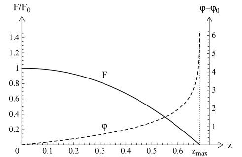
FIG. 1.: Reconstructed $F(z)$ [i.e., Brans-Dicke scalar $\Phi_{\rm BD}(z)$] and Einstein-frame scalar $\varphi$ as functions of the Jordan-frame (i.e., observed) redshift $z$, for the maximum value of $|\alpha_{0}|$ allowed by solar-system experiments, and for a vanishing potential. The helicity-0 degree of freedom $\varphi$ diverges at $z_{\rm max}\approx 0.68$.

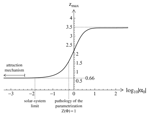
FIG. 2.: Maximum redshift $z$ consistent with the positivity of energy of both the graviton and the scalar field, as a function of the parameter $|\alpha_{0}|$. This figure corresponds to the case of a vanishing scalar-field potential, and we fit the exact $H(z)$ predicted by general relativity plus a cosmological constant (GR $+\Lambda$).

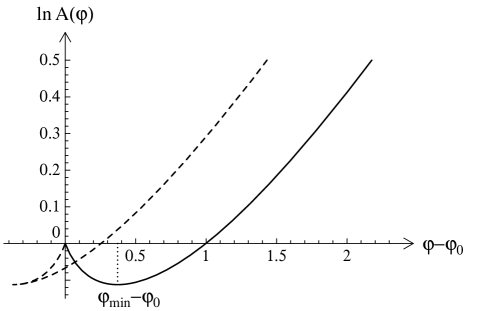
FIG. 3.: Two versions of the reconstructed coupling function $\ln A(\varphi)$ for $|\alpha_{0}|=1$, the dashed one looking bi-valued, but the (single-valued) solid one giving the same predicted $H(z)$. This figure still corresponds to the case of a vanishing scalar-field potential, and we fit the exact $H(z)$ predicted by GR $+\Lambda$.

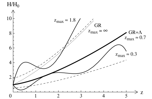
FIG. 4.: Random deformations of the $H(z)$ predicted by GR $+\Lambda$ (with $\Omega_{\Lambda,0}=0.7$), and corresponding maximum value of the redshift $z$ consistent with the positivity of energy. The dashed lines indicate the region in which random points have been chosen at regular intervals of $z$. The thin solid lines correspond to two polynomial fits of such random points. Note that they can differ from the GR $+\Lambda$ curve even more than the dashed lines. The dotted line labeled simply “GR” corresponds to a vanishing cosmological constant $\Lambda$. Such a bias of the GR $+\Lambda$ curve changes $z_{\rm max}$ much more that the random noise we considered.

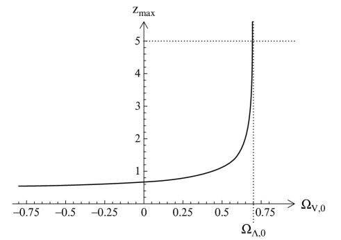
FIG. 5.: Maximum redshift $z$ consistent with the positivity of energy, as a function of the value of a constant potential $V$ (case of a massless helicity-0 degree of freedom $\varphi$).

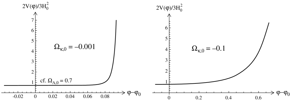
FIG. 6.: Minimally coupled model $F=1$ in a spatially closed FRW universe, respectively for $\Omega_{\kappa,0}=-10^{-3}$ (left panel) and $\Omega_{\kappa,0}=-0.1$ (right panel). In both cases, the potential $V(\varphi)$ is analytically given by Eq. (VI C 1). Note that the reconstructed potential does not have a “natural” shape if $|\Omega_{\kappa,0}|$ is too small: The present value of $\Omega_{\Lambda,0}$ is not explained by a quintessence mechanism, and the corresponding scalar-tensor theory is basically equivalent to GR $+\Lambda$. On the contrary, if $|\Omega_{\Lambda,0}|$ is large enough, the potential has a nice smooth shape, and its present value (at $\varphi-\varphi_{0}=0$ on the figure) basically corresponds to the observed $\Omega_{\Lambda,0}$.

- [1] S. Perlmutter, G. Aldering, M. Della Valle et al., Nature 391, 51 (1998); S. Perlmutter, G. Aldering, G. Goldhaber et al., Astroph. J., 517, 565 (1999).
- [2] P.M. Garnavich, R.P. Kirshner, P. Challis et al., Astrophys. J. Lett. 493, L53 (1998); A.G. Riess, A.V. Philipenko, P. Challis et al., Astron. J. 116, 1009 (1998).
- [3] P. de Bernardis et al., Nature 404, 955 (2000).
- [4] S. Hanany et al., astro-ph/0005123; A. Balbi et al., astro-ph/0005124.
- [5] N.A. Bahcall, J.P. Ostriker, S. Perlmutter, and P.J. Steinhardt, Science, 284, 1481 (1999).
- [6] V. Sahni and A.A. Starobinsky, IJMPD, to appear (2000); astro-ph/9904398.
- [7] M. Chevallier and D. Polarski, submitted, gr-qc/0009008
- [8] R.R. Caldwell, R. Dave, and P.J. Steinhardt, Phys. Rev. Lett. 80, 1582 (1998).
- [9] B. Ratra and P.J.E. Peebles, Phys. Rev. D 37, 3406 (1988).
- [10] P.G. Ferreira and M. Joyce, Phys. Rev. D 58, 023503 (1998); Phys. Rev. Lett. 79, 4740 (1998).
- [11] I. Zlatev, L. Wang and P.J. Steinhardt, Phys. Rev. Lett. 82, 896 (1999).
- [12] A.D. Liddle and R.J. Scherrer, Phys. Rev. D 59, 0223509, (1998).
- [13] C. Kolda and D.H. Lyth, Phys. Lett. B 458, 197 (1999).
- [14] A.A. Starobinsky, JETP Lett. 68, 757 (1998); Gravit. & Cosmol. 4 (Suppl.), 88 (1998).
- [15] D. Huterer and M.S. Turner, Phys. Rev. D 60, 081301 (1999); T. Nakamura and T. Chiba, Mon. Not. Roy. Ast. Soc. 306, 696 (1999).
- [16] T.D. Saini, S. Raychaudhury, V. Sahni, and A.A. Starobinsky, astro-ph/9910231.
- [17] R.R. Caldwell, astro-ph/9908168.
- [18] C.M. Will, Theory and Experiment in Gravitational Physics, (Cambridge University Press, Cambridge, England, 1993).
- [19] T. Damour and G. Esposito-Farèse, Class. Quant. Grav. 9, 2093 (1992).
- [20] T. Damour and G. Esposito-Farèse, Phys. Rev. D 53, 5541 (1996).
- [21] T. Damour and G. Esposito-Farèse, Phys. Rev. D 54, 1474 (1996).
- [22] C.M. Will, Phys. Rev. D 50, 6058 (1994).
- [23] T. Damour and G. Esposito-Farèse, Phys. Rev. D 58, 042001 (1998).
- [24] M. Gasperini and G. Veneziano, Astropart. Phys. 1 (1993) 317; Mod. Phys. Lett. A8 (1993) 3701.
- [25] T. Damour and K. Nordtvedt, Phys. Rev. Lett. 70, 2217 (1993); Phys. Rev. D 48, 3436 (1993).
- [26] D.I. Santiago, D. Kalligas, and R.V. Wagoner, Phys. Rev. D 58, 124005 (1998).
- [27] T. Damour and B. Pichon, Phys. Rev. D 59, 123502 (1999).
- [28] A. Navarro, A. Serna, and J.M. Alimi, Phys. Rev. D 59, 124015 (1999).
- [29] J.P. Uzan, Phys. Rev. D 59, 123510 (1999).
- [30] T. Chiba, Phys. Rev. D 60, 083508 (1999).
- [31] X. Chen and M. Kamionkowski, Phys. Rev. D 60, 104036 (1999).
- [32] F. Perrotta, C. Baccigalupi, and S. Matarrese, astro-ph/9906066.
- [33] D.J. Holden and D. Wands, gr-qc/9908026.
- [34] N. Bartolo and M. Pietroni, hep-ph/9908521.
- [35] E. Gaztanaga and J.A. Lobo, astro-ph/0003129.
- [36] B. Boisseau, G. Esposito-Farèse, D. Polarski, and A.A. Starobinsky, Phys. Rev. Lett. 85 (2000) 2236.
- [37] C.W. Misner, K.S. Thorne, J.A. Wheeler, Gravitation (San Francisco, Freeman, 1973).
- [38] P.G. Bergmann, Int. J. Theor. Phys. 1, 25 (1968); K. Nordtvedt, Astrophys. J. 161, 1059 (1970); R. Wagoner, Phys. Rev. D 1, 3209 (1970).
- [39] T.M. Eubanks et al., Bull. Am. Phys. Soc., Abstract #K 11.05 (1997).
- [40] J.O. Dickey et al., Science 265, 482 (1994); J.G. Williams, X.X. Newhall, and J.O. Dickey, Phys. Rev. D 53, 6730 (1996).
- [41] P. Fiziev, gr-qc/9911037.
- [42] A.S. Eddington, The Mathematical Theory of Relativity, (Cambridge University Press, Cambridge, 1923).
- [43] B.M. Barker, Astrophys. J. 219, 5 (1978).
- [44] J.M. Bardeen, Phys. Rev. D 22, 1882 (1980).
- [45] L. Amendola, Phys. Rev. D 60, 043501 (1999).
- [46] J. Weller and A. Albrecht, astro-ph/0008314; I. Maor, R. Brustein and P.J. Steinhardt, astro-ph/0007297; T. Chiba and T. Nakamura, astro-ph/0008175.
- [47] T. Damour and A. Polyakov, Nucl. Phys. B423, 532 (1994); Gen. Rel. Grav. 26, 1171 (1994).