Holonomy in the Schwarzschild-Droste Geometry

Abstract

Parallel transport of vectors in curved spacetimes generally results in a deficit angle between the directions of the initial and final vectors. We examine such holonomy in the Schwarzschild-Droste geometry and find a number of interesting features that are not widely known. For example, parallel transport around circular orbits results in a quantized band structure of holonomy invariance. We also examine radial holonomy and extend the analysis to spinors and to the Reissner-Nordström metric, where we find qualitatively different behavior for the extremal ($Q=M$) case. Our calculations provide a toolbox that will hopefully be useful in the investigation of quantum parallel transport in Hilbert-fibered spacetimes.

PACS: 04.20-q, 04.70Bw, 04.20-Cv
Keywords: Holonomy, Black holes, Schwarzschild.

1 Introduction

Holonomy transformations measure the change in direction acquired by a vector under parallel transport around a closed loop, or between two distinct points via different paths. To be more precise, if $T_{p}$ is the tangent space to a manifold at the point $p$, then a holonomy transformation is a set of linear maps from $T_{p}$ into itself, induced by parallel transfer around closed paths based on $p$. Each such path defines an element of the holonomy group, determining the deficit angle between the initial and final positions of a vector after such parallel transport. It is a global property of the manifold and as such can also serve as a tool for the global classification of spacetimes in a manner similar to but distinct from the local Petrov and Segre type classifications. In this regard, the holonomy group structure of various (simply connected) spacetimes has received exhaustive study [1]. From the point of view of its intrinsic mathematical interest as well, holonomy in various spacetimes has been extensively examined, although in more “exotic” settings, such as cylindrically symmetric spacetimes or cosmic string backgrounds (see [2, 3] and references therein). Holonomy properties of one of the most fundamental and important spacetimes, the Schwarzschild-Droste geometry, have received virtually no attention in the literature. To the best of our knowledge, only one paper [4] reports any results in the Schwarzschild-Droste background, and this as a special case of the rotating (Kerr) solution.

Apparently, the neglect of the Schwarzschild-Droste spacetime is for a simple reason: When asked whether a vector parallely transported in an ‘equatorial’ orbit around a Schwarzschild-Droste (SD) black hole will manifest a deficit angle after completing a full circle, most relativists answer, “No.” The intuitive response evidently relies on one’s sense of spherical symmetry—nothing changes during completion of the orbit—and on the fact that around the equator of an ordinary two-sphere the phase change is indeed zero. Here, however, is a striking case where intuition fails. It is easy to show, as we do below, that parallel transport in a circular orbit around a SD black hole definitely results in a nonzero deficit angle—the vector has changed direction. The first and most important point to be made regarding holonomy in the SD geometry, therefore, is that nonzero holonomy exists and consequently provides a gravitational analog to the Aharonov-Bohm effect [5, 6]. (Strictly speaking, the Aharonov- Bohm effect takes place in a region where there is no electromagnetic field, whereas the SD spacetime certainly contains a gravitational field. A closer analogy would be an asymptotically flat, cylindrically symmetric space time, such as that produced by cosmic strings [3], which contains a conical singularity.)

Beginning with the simple calculation for circular orbits, we explore holonomy along a variety of paths in the SD geometry, for both geodesic and non geodesic motion. We find several surprising results. Although a few of these are presented in [4], the majority are not and, in any case, none of them appear to be widely known. We then carry out the calculations in loop variables, extend the results to spinors and extremal Reissner-Nordström geometry, and finally discuss some features that may bear on future calculations involving “quantum holonomy.”

2 Two-sphere and Schwarzschild-Droste metric

It is an elementary exercise to show (see [7]) that parallel transporting a vector ${\bf A}=A^{\phi}{\bf{\hat{e}_{\phi}}}+A^{\theta}{\bf{\hat{e}_{\theta}}}$ along a constant $\theta$ curve on the surface of an ordinary two-sphere, leads to

$$A^{\phi} = \frac{\alpha\cos(\phi\ \cos\theta)-\beta\sin(\phi\ \cos\theta)}{\sin\theta}$$

$$A^{\theta} = \alpha\sin(\phi\ \cos\theta)+\beta\cos(\phi\ \cos\theta),$$ (2.1)

where $\alpha$ and $\beta$ are integration constants. Note that when $\phi=0$ we have $A^{\phi}=\alpha/sin\theta$ and $A^{\theta}=\beta$, and that after completion of a full circle

$$A^{\phi} = \frac{\alpha\cos(2\pi\ \cos\theta)-\beta\sin(2\pi\ \cos\theta)}{\sin\theta}$$

$$A^{\theta} = \alpha\sin(2\pi\ \cos\theta)+\beta\cos(2\pi\ \cos\theta).$$ (2.2)

We see that on the equator ($\theta=\pi/2$) or at the north pole ($\theta=0$), parallel transport has no effect on the components of ${\bf A}$, but that for arbitrary $\theta$, $A^{\phi}(2\pi)$ and $A^{\phi}(0)$ differ, similarly for $A^{\theta}(2\pi)$ and $A^{\theta}(0)$. As mentioned, it is perhaps the zero result on the equator that helps to lead one’s intuition astray and to predict that the same will hold for the SD geometry. However, this is not the case. We begin by setting the scene in which we will work. Let $({\cal M},{\bf g})$ be a four-dimensional Lorentzian manifold with Reissner-Nordström metric. The line element is, as usual,

$$ds^{2}=-(1-\frac{2M}{r}+\frac{Q^{2}}{r^{2}})dt^{2}+(1-\frac{2M}{r}+\frac{Q^{2}}{r^{2}})^{-1}dr^{2}+r^{2}(d\theta^{2}+\sin^{2}\theta d\phi^{2}),$$ (2.3)

where $Q$ is the charge and $M$ the mass. Most of the paper will be concerned solely with the SD case, which is obtained by setting $Q=0$. In section 7, however, we will want to compare a few features of the Schwarzschild-Droste geometry with the Reissner-Nordström case so it will prove useful to have the relevant quantities available. For convenience we will carry out calculations in an orthonormal tetrad. The obvious choice is defined by the dual 1-form basis $\omega^{a}=\omega_{\;i}^{a}(x^{j})dx^{i}$, where

$$\omega^{0} = \omega^{t}=(1-\frac{2M}{r}+\frac{Q^{2}}{r^{2}})^{1/2}dt,$$

$$\omega^{1} = \omega^{r}=(1-\frac{2M}{r}+\frac{Q^{2}}{r^{2}})^{-1/2}dr,$$

$$\omega^{2} = \omega^{\theta}=r\,d\theta,$$

$$\omega^{3} = \omega^{\phi}=r\sin\theta\,d\phi.$$ (2.4)

The connection forms are defined by $d\omega_{\;}^{a}=-\omega_{\;b}^{a}(x^{j})\wedge\omega_{\;}^{b}.$ For the above 1-forms, we can choose the connection forms [8] as

$$\omega_{\;r}^{t} = (\frac{M}{r^{2}}-\frac{Q^{2}}{r^{3}})(1-\frac{2M}{r}+\frac{Q^{2}}{r^{2}})^{-1/2}\omega^{t}=\omega_{\;t}^{r},$$

$$\omega_{\;r}^{\theta} = \frac{1}{r}(1-\frac{2M}{r}+\frac{Q^{2}}{r^{2}})^{1/2}\omega^{\theta}=-\omega_{\;\theta}^{r}\;,$$

$$\omega_{\;r}^{\phi} = \frac{1}{r}(1-\frac{2M}{r}+\frac{Q^{2}}{r^{2}})^{1/2}\omega^{\phi}=-\omega_{\;\phi}^{r}\;,$$

$$\omega_{\;\theta}^{\phi} = \frac{\cot\theta}{r}\omega^{\phi}=-\omega_{\;\phi}^{\theta}.$$ (2.5)

Let ${\bf A}=A^{\mu}\partial_{\mu}$ be some vector field on ${\cal M}$ i.e., a section of the tangent bundle of ${\cal M}$. By requiring that $\bf A$ be a parallel section of the tangent bundle we can write the parallel transport equation in a coordinate-free way as

$$dA^{\mu}+\omega^{\mu}_{\beta}A^{\beta}=0.$$ (2.6)

Using the results of eqs.(2.4) and (2.5) we write eq.(2.6) (for the Reissner-Nordström geometry) in components as

$$dA^{t}+(M/r^{2}-Q^{2}/r^{3})A^{r}dt= 0$$ ,

$$dA^{r}+(M/r^{2}-Q^{2}/r^{3})A^{t}dt-(1-2M/r+Q^{2}/r^{2})^{\frac{1}{2}}A^{\theta}d\theta$$

$$-(1-2M/r+Q^{2}/r^{2})^{\frac{1}{2}}A^{\phi}d\phi= 0$$ ,

$$dA^{\theta}+(1-2M/r+Q^{2}/r^{2})^{\frac{1}{2}}A^{r}d\theta= 0$$ ,

$$dA^{\phi}+(1-2M/r+Q^{2}/r^{2})^{\frac{1}{2}}A^{r}d\phi= 0$$ . (2.7)

In what follows we consider some special curves along which ${\bf A}$ is parallel transported. Unless explicitly stated to the contrary we will restrict ourselves to the Schwarzschild solution for which $Q=0$.

3 Circular orbits

Due to the spherical symmetry of the SD solution, we may take any circular orbit to be equatorial, i.e., $\theta=\pi/2$. Then, since $r=const$ for these orbits we have for the tangent vector $X^{\nu}=(X^{t},0,0,X^{\phi})=(dt/d\lambda,0,0,d\phi/d\lambda)$. Parameterizing such curves by $\phi$ and assuming constant speed with $\mu\equiv dt/d\phi>c^{-1}$ we find from eqs.(2.7) with $d\theta/d\phi=0$,

$$dA_{\;\ }^{t}/d\phi + (\frac{M}{r^{2}}A^{r})\mu=0,$$ (3.1)

$$dA_{\;\ }^{r}/d\phi + \frac{M}{r^{2}}A^{t}\mu-(1-\frac{2M}{r})^{1/2}A^{\phi}=0,$$ (3.2)

$$dA_{\;\ }^{\theta}/d\phi = 0,$$ (3.3)

$$dA_{\;\ }^{\phi}/d\phi + (1-\frac{2M}{r})^{1/2}A^{r}=0.$$ (3.4)

Equation (3.3) is of course trivial and merely reflects the constancy of $A^{\theta}$. The other equations may be easily integrated to give

$$A^{r}(\phi) = \alpha\sin\omega\phi+\beta\cos\omega\phi$$ (3.5)

$$A^{t}(\phi) = \frac{\mu M}{\omega r^{2}}(\alpha\cos\omega\phi-\beta\sin\omega\phi)+\gamma,$$ (3.6)

$$A^{\phi}(\phi) = \frac{1}{\omega}(1-\frac{2M}{r})^{1/2}(\alpha\cos\omega\phi-\beta\sin\omega\phi)+\delta,$$ (3.7)

where the “frequency” $\omega$ is given by

$$\omega^{2}\equiv 1-\frac{2M}{r}-\mu^{2}\frac{M^{2}}{r^{4}},$$ (3.8)

and$\gamma$ and $\delta$ are integration constants. Note that at $r=2M$, $\omega^{2}$ is negative, whereas for fixed $\mu^{2}M^{2}$, $\omega^{2}\rightarrow 1$ as $r\rightarrow\infty$. Thus $\omega^{2}$ will change sign at some $r=r_{crit}$, which depends on the dimensionless parameter $\mu^{2}M^{2}/r^{4}$. The oscillatory solutions above are valid in the region $r>r_{crit}$. The constants $\gamma$ and $\delta$ are not independent. Substituting the solutions back into the differential equations shows that $\delta=(1-2M/r)^{-1/2}(M\mu/r^{2})\gamma$. Also note that for $r<r_{crit}$, the solutions are exponential, in which case the trigonometric functions in (3.5) are replaced by the corresponding hyperbolic function. Eqs. (3.6) and (3.7), obtained by integrating (3.5), must be changed accordingly.

3.1 Constant-time circles

The surprising properties of holonomy in the SD geometry can most easily be seen by examining constant-time orbits. In this case, $\mu=0$ and so $r_{crit}=2M$. Thus $\omega^{2}$ is always positive and the oscillatory solutions are relevant. Suppose $\phi=0$ at the start. After $n$ loops $\phi=2\pi n$. $A^{t}=\gamma$ always and $A^{\theta}=constant$. The remaining two components of $\bf A$ are

$$A_{\ }^{\phi}(2n\pi) = \alpha\cos[(1-\frac{2M}{r})^{1/2}2n\pi]-\beta\sin[(1-\frac{2M}{r})^{1/2}2n\pi],$$ (3.9)

$$A_{\;\ }^{r}(2n\pi) = \alpha\sin[(1-\frac{2M}{r})^{1/2}2n\pi]+\beta\cos[(1-\frac{2M}{r})^{1/2}2n\pi].$$ (3.10)

These equations show clearly that nonzero holonomy exists on equatorial orbits in the SD geometry. We point out that the expressions are consistent with the results for the two-sphere in flat space. As $r\rightarrow\infty$, the holonomy goes to zero. However, for finite $r$, a deficit angle exists after transport through and angular displacement of $2\pi$ except when $n(1-\frac{2M}{r})^{1/2}$ is equal to an integer! It is this “quantization” of holonomy that is initially striking. Nevertheless, it is true and can be understood as follows: Suppose that on an orbit of radius $r_{1}$, the holonomy “closes” and there is no deficit. At another orbit $r_{2}$ slightly farther out, there must be a nonzero holonomy because the space between the two orbits is curved and according to the Gauss-Bonnet theorem, the deficit angle is the integral of the Gaussian curvature over the area enclosed by the two curves. Had we considered only the holonomy intrinsic to the SD two-sphere, the result would have been the same as for the two-sphere in Euclidean space—zero. The difference is that we are here considering parallel transport in the full space, which is the space relevant to local physics, and which is curved. The quantization condition for holonomy invariance implies that

$$r=\frac{2M}{1-m^{2}/n^{2}},$$ (3.11)

with $m$ a non-zero integer. Since we require $r>2M$, we must have $0<m^{2}/n^{2}<1$. For fixed $m$, then, there is a minimum $n$ that will give holonomy invariance. In particular, no invariance after $2\pi$ exists for $m=1$. After two loops invariance is possible at $r=8M/3$. In Table I we give examples of holonomy invariance for various values of $m$ and $n$.

n=1 n=2 n=3 n=4

m=1 x 2.667 2.25 2.133

m=2 x x 3.6 2.667

m=3 x x x 6.4

m=4 x x x x

Table 1: The table gives the radii $r$ (in units of $M$) at which holonomy invariance for constant-time circular orbits is achieved for integer $m$ and $n=$ number of circuits. An $x$ indicates that no invariance is possible for those values of $m$ and $n$.

3.2 Timelike circles

We consider now timelike circles. The tetrad components of the tangent vector are given by $X^{a}=(\mu(1-2M/r)^{\frac{1}{2}},0,0,r)$. For timelike curves we require the squared magnitude to be less than zero, or $r^{3}+2M\mu^{2}-\mu^{2}r<0$. For such circles with radius $r>r_{crit}$, we have $A^{r}(0)=\beta,\ A^{t}(0)=(\mu M/\omega r^{2})\alpha+\gamma$ and $A^{\phi}(0)=\omega^{-1}(1-2M/r)^{1/2}\alpha+\delta$. Hence from (3.5)-(3.7) after $n$ loops:

$$\Delta A^{r}(2n\pi) = \alpha\sin\omega 2n\pi+\beta(\cos\omega 2n\pi-1),$$ (3.12)

$$\Delta A^{t}(2n\pi) = \frac{\mu M}{\omega r^{2}}(\alpha(\cos\omega 2n\pi-1)-\beta\sin\omega 2n\pi),$$ (3.13)

$$\Delta A^{\phi}(2n\pi) = \frac{1}{\omega}(1-\frac{2M}{r})^{1/2}(\alpha(\cos\omega 2n\pi-1)-\beta\sin\omega 2n\pi)$$ (3.14)

$$\Delta A_{\;}^{\theta}(2n\pi) = 0.$$

where $\Delta$ represents the difference in the components before and after transport. For invariance all the $\Delta$’s must vanish, which is achieved when $\omega 2\pi n$ is an integer. However, since $\omega$ depends in a nontrivial way on $\mu^{2}M^{2}/r^{4}$, we will only examine the case of greatest interest.

3.3 Circular Geodesics

A geodesic is obtained by parallel transporting a tangent vector along its integral curve. Note for the tangent vector above that $X^{r}=0$. Eqs. (3.1)-(3.4) show that for any vector with $A^{r}=0$, all components are constant with

$$A^{\phi}=\mu\frac{M}{r^{2}}(1-\frac{2M}{r})^{-1/2}\,A^{t}.$$

Applying this condition to $X$ itself yields

$$\mu\frac{M}{r^{2}}(1-\frac{2M}{r})^{-1/2}=X^{\phi}/X^{t}=r/((1-\frac{2M}{r})^{1/2}\mu),$$

which gives

$$\mu^{2}M=r^{3}.$$ (3.15)

This is Kepler’s third law for relativistic orbits. Now, the magnitude of $X$ is $3(1-r/3M)r^{2}$. Thus a circular geodesic is timelike for $r>3M$, spacelike for $r<3M$ and null for $r=3M$, as required (this is the last stable orbit for photons). Furthermore, we see that for circular geodesics the Kepler condition implies $\omega^{2}=1-3M/r$, which means that $r_{crit}=3M$. In the context of the so-called optical geometry (see [9, 10] and references therein), this surprising result is perhaps not so surprising. In the optical metric (where the usual SD spatial metric is multiplied by $(1-2M/r)^{-1}$, a conformal rescaling), all dynamical effects of circular motion reverse at $r=3M$, for example the direction of centrifugal force and the direction of precession of gyroscopes. To this list we may add another effect: the change of parallely propagated solutions along circular geodesics from oscillatory to exponential.

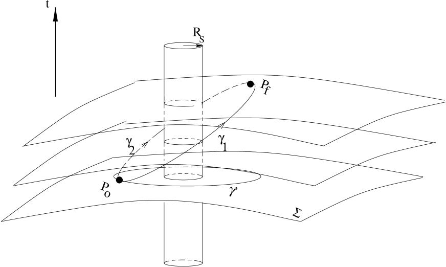
Figure 1: Circular geodesics in Schwarzschild spacetime. $P_{0}$ is the initial point, $P_{f}$ is the final point; $\Sigma$ represents the initial hypersuface and $\gamma_{1}$ and $\gamma_{2}$ circular geodesics.

The expression for $\omega$ allows us to compute holonomy invariance for geodesic paths whose spatial projections are circular orbits (Fig. 1). In this case, invariance is achieved when

$$(1-\frac{3M}{r})^{1/2}n=m.$$ (3.16)

Clearly the condition that $r>2M$ puts restrictions on the allowed values of $n$ that give holonomy invariance. In particular, no holonomy invariance exists for $n=1$; for $n=2$, $r=12/3M$ gives invariance after transport through an angle $2\pi$. Table II gives other values of holonomy for circular geodesics.

n=1 n=2 n=3 n=4

m=1 x 4 3.375 3.2

m=2 x x 5.4 4

m=3 x x x 9.6

m=4 x x x x

Table 2: The table gives the radii $r$ (in units of $M$) at which holonomy invariance for circular geodesics is achieved for integer $m$ and $n=$ number of circuits. As in Table I. an $x$ indicates that no invariance is possible for those values of $m$ and $n$.

4 Radial Holonomy

In the case of radial paths, we take the tangent vector to be $X^{\mu}=[X^{t},X^{r},0,0]$. We may choose $t$ or $r$ to be the curve parameter $\lambda$, and thus may set either $X^{t}$ or $X^{r}$ to 1. However, in this case one should avoid putting $dt/dr=constant$, or vice versa, since this will in general not be true for radial geodesics. Let us now specialize to radial null geodesics. To find them, note that the tetrad components of the tangent vector are

$$X^{a}={\Bigl{(}}(1-\frac{2M}{r})^{1/2}X^{t},(1-\frac{2M}{r})^{-1/2}X^{r},0,0{\Bigr{)}},$$ (4.1)

with magnitude

$$X^{2}=-(1-\frac{2M}{r})(X^{t})^{2}+(1-\frac{2M}{r})^{-1}(X^{r})^{2}.$$

This vector is null if and only if $(1-\frac{2M}{r})(X^{t})^{2}=(1-\frac{2M}{r})^{-1}(X^{r})^{2}$, which implies

$$(X^{t})^{2}=(1-\frac{2M}{r})^{-2}(X^{r})^{2}.$$ (4.2)

With a curve parameter $r$, eqs.(2.7) reduce to two nontrivial equations

$$\frac{dA^{t}}{dr}+\frac{M}{r^{2}}(1-\frac{2M}{r})^{-1}A^{r} = 0,$$ (4.3)

$$\frac{dA^{r}}{dr}+\frac{M}{r^{2}}(1-\frac{2M}{r})^{-1}A^{t} = 0,$$ (4.4)

which are easily integrated to give the general solution

$$A^{t} = c_{1}(1-2M/r)^{-\frac{1}{2}}+c_{2}(1-2M/r)^{\frac{1}{2}},$$ (4.5)

$$A^{r} = c_{1}(1-2M/r)^{-\frac{1}{2}}-c_{2}(1-2M/r)^{\frac{1}{2}}.$$ (4.6)

The integration constants $c_{1}$ and $c_{2}$ may be fixed as $1$ and $0$ respectively by imposing that $A^{t}=X^{t}$ and $A^{r}=X^{r}$. This yields

$$A^{t}=A^{r}=(1-2M/r)^{-\frac{1}{2}}.$$ (4.7)

Turning to constant $r,\theta,\phi$ curves, we now have $X^{r}=0$ and $t$ may be taken as the curve parameter. The solutions

$$A^{t}(t) = A^{t}(0)\cosh(\frac{M}{r^{2}}t)-A^{r}(0)\sinh(\frac{M}{r^{2}}t),\;$$

$$A^{r}(t) = A^{r}(0)\cosh(\frac{M}{r^{2}}t)-A^{t}(0)\sinh(\frac{M}{r^{2}}t),$$ (4.8)

with $A^{\theta}$ and $A^{\phi}$ constant are easily found from eqs.(2.7) by setting $d\phi=0$ and integrating. These expressions may then be used to construct holonomy along sample paths. For example, consider a constant $r,\phi$ curve as above. We transport a vector $A=(A^{t}(0),A^{r}(0),A^{\theta}(0),A^{\phi}(0))$ along a radial null geodesic from a point A at a radius $r_{o}$ inward to a point B at $r=r_{1}$, then outward along a radial null geodesic to $r=r_{0}$ again to a point C, as in Fig. 2. The radial contributions cancel and we are left with the holonomic change

$$\Delta A^{t} = A^{t}(0){\Bigl{(}}\cosh(\frac{M}{r_{o}^{2}}t_{C})-1{\Bigr{)}}-A^{r}(0)\sinh(\frac{M}{r_{o}^{2}}t_{C}),$$

$$\Delta A^{r} = A^{r}(0){\Bigl{(}}\cosh(\frac{M}{r_{o}^{2}}t_{C})-1{\Bigr{)}},$$ (4.9)

where we have taken $t_{A}=0$. Note that as $r_{0}\rightarrow\infty$ the change in the vector due to parallel transport vanishes. Indeed this is to be expected from the asymptotic flatness of the Schwarzschild spacetime. This result can be found in [4]. However, we emphasize that the $r,\phi=constant$ path is far from generic; any spaceship on such an orbit would have to fire rockets to remain in position and thus this is definitely not geodesic motion. A more “realistic” path would be a wedge, bounded by two circular orbits at radii $r_{0}$ and $r_{1}$ and two radial geodesics, as in Fig. 3.

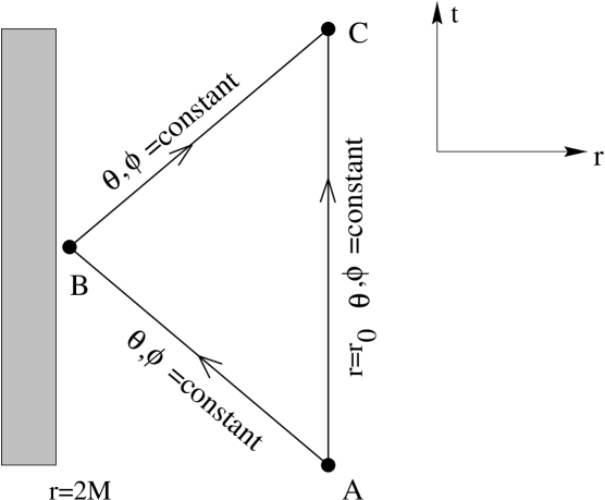
Figure 2: Spacetime diagram for a path traversed radially inward from a point $A$ at some finite radius $r=r_{0}$ to a point $B$ neighborhood of the Schwarzschild radius and then radially outward to $C$, at the radius $r_{0}$. We assume that the radial paths, $AB$ and $BC$ are radial ingoing and outgoing geodesics respectively.

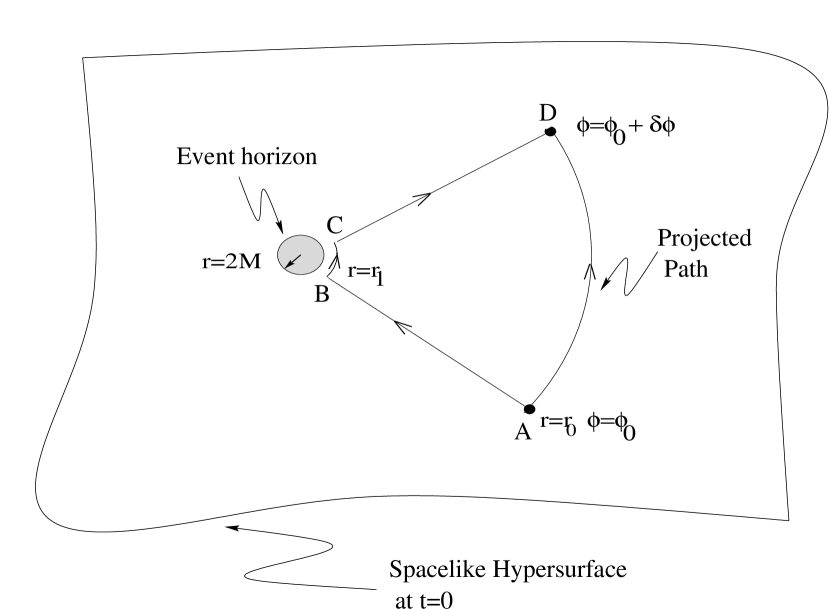
Figure 3: Projection of a ‘wedge shaped’ path onto the initial spatial hypersurface.

Again, the radial contributions cancel and if one compares the vector transported directly from A to D with one transported around the loop from A to B to C to D, one gets holonomy for, say, the $A^{r}$ component (setting $\alpha=0$ which yields $\beta=A^{r}(0)$)

$$\Delta A^{r}=A^{r}(0)\left\{\cos(\omega_{0}\phi)-\cos[(1-\frac{3M}{r_{1}})^{1/2}\phi]\right\},$$ (4.10)

if $r_{0},r_{1}>r_{crit}$. We have assumed for illustration that one circular orbit is a geodesic but not the other because, in general. both cannot be geodesic. That is, although the angles are the same, the time taken to traverse the outer orbit is exponentially longer than the time taken to traverse the inner orbit. This in turn is because the time taken for photons to traverse the radial null geodesics is given by

$$t=|r_{*}|=\int\frac{dr}{(1-\frac{2M}{r})^{1/2}}.$$

Consequently, $t_{0}$ is not independent of $t_{1}$. However, for geodesics, Kepler’s law determines the time taken to traverse a given angle; thus when both orbits are geodesics the system is over-determined. With $\omega$ given by (3.8), equating the arguments in (4.10) gives for holonomy invariance modulo $2\pi$

$$r_{1}=\frac{3r_{0}^{4}}{2r_{0}^{3}+\mu^{2}M}.$$

If $\mu^{2}M$ is small compared to $r_{0}^{3}$, this yields $r_{1}=3/2r_{0}$. Note that if $r_{0}$ is taken to be a geodesic orbit, then $\mu^{2}M=r_{0}^{3}$ and $r_{1}=r_{0}$, showing that in this limit no holonomy invariance is possible modulo $2\pi$ unless the two geodesic orbits are the same. For higher number of circuits invariance is possible.

In Section 8 we will discuss possible applications of holonomy. Before doing this, however, it will be helpful to motivate the discussion by recovering some of the previous results via the loop formalism and for spinors, and investigating a few properties of holonomy in the Reissner-Nordström background.

5 Loop formulation

As is clear from the previous discussion, the result of parallel transport is path dependent. This may be stated slightly more rigorously as follows: Let ${\cal M}$ be some $n$-dimensional manifold (which we shall choose as our Schwarzschild background). For each closed curve $\gamma:[0,1]\rightarrow{\cal M}$ with base point $p$, parallel transport associates some $GL(n,{\bf R})$-valued operator $U(\gamma)$ acting on $T_{p}$ called the holonomy. The concept of holonomy has appeared in many guises in physics from lattice gauge theories [11] to loop quantum gravity [12] (see also [4, 2, 3] for further details) with just as many aliases. Thus it is known, for example, as the Wu-Yang phase factor in particle physics. The holonomy associated with the parallel transport around $\gamma$ is a linear map from the tangent space at a point $p\in{\cal M}$ into itself, realized by the path-ordered exponential

$$U(\gamma)=P\,e^{-\int_{\gamma}\,\Gamma_{\mu}dx^{\mu}},$$ (5.1)

where $\Gamma_{\mu}$ is the tetradic connection on ${\cal M}$. Choosing ${\cal M}$ to be a $4$-dimensional Lorentzian manifold with Schwarzschild metric we get,

$$\Gamma_{\mu}=\left(\begin{array}[]{llll}0&\Gamma_{\;rt}^{t}&0&0\\ \Gamma_{\;tt}^{r}&0&\Gamma_{\;\theta\theta}^{r}&\Gamma_{\;\phi\phi}^{r}\\ 0&\Gamma_{\;r\theta}^{\theta}&0&\Gamma^{\theta}_{\phi\phi}\\ 0&\Gamma_{\;r\phi}^{\phi}&\Gamma^{\phi}_{\theta\phi}&0\end{array}\right)$$ (5.2)

where the connection coefficients are as derived from (2.5).

To illustrate an explicit representation of $U(\gamma)$ consider circular orbits, $\Gamma_{\mu}dx^{\mu}=\Gamma_{t}dt+\Gamma_{\phi}d\phi$. Clearly the matrix elements $\Gamma_{\;\theta\theta}^{r}$ and $\Gamma_{\;r\theta}^{\theta}$ of (5.2) vanish. With $\mu\equiv dt/d\phi$ as before, we can write $\int\Gamma_{t}dt+\Gamma_{\phi}d\phi=2\pi[\Gamma_{t}\mu+\Gamma_{\phi}]\equiv 2\pi\Gamma$. We then need to evaluate

$$U=e^{-\int\Gamma_{\mu}dx^{\mu}}=e^{-2\pi\Gamma}=1-2\pi\Gamma+\frac{(2\pi\Gamma)^{2}}{2!}-\frac{(2\pi\Gamma)^{3}}{3!}+....$$ (5.3)

A little algebra shows that $\Gamma^{3}=-S^{2}\Gamma$, where $S^{2}\equiv(\Gamma_{\;r\phi}^{\phi})^{2}-\mu^{2}(\Gamma_{\;rt}^{t})^{2}$ in terms of which the Taylor series (5.3) becomes

$$U=1-\frac{\Gamma}{S}\sin(2\pi S)+\frac{\Gamma^{2}}{S^{2}}(1-\cos(2\pi S)).$$ (5.4)

We see, somewhat unexpectedly, that $S^{2}=1-\frac{2M}{r}-\frac{M^{2}\mu^{2}}{r^{4}}=\omega^{2}$. The final vector ${\bf A_{f}}$ after parallel transport is given merely by ${\bf U\cdot A_{o}}=U^{\alpha}\;_{\beta}A_{o}^{\beta}$. Thus, the deficit angle between the initial and final vector is simply ${\bf A_{o}\cdot A_{f}=A_{o}\cdot U\cdot A_{o}}=|A_{o}||A_{f}|\cos\chi$, where $\chi$ is the deficit angle. Thus, in general, ${\bf\hat{A}_{o}\cdot\hat{A}_{f}}=\cos\chi$ where ${\bf\hat{A}_{o}}$ and ${\bf\hat{A}_{f}}$ are now unit vectors. Given $U$ as in (5.4) we find ${\bf\hat{A}_{o}\cdot\hat{A}_{f}}=\cos(2\pi S)$. For constant- time circles, $\mu=0$, which immediately gives ${\bf\hat{A}_{o}\cdot\hat{A}_{f}}=\cos(2\pi(1-2M/r)^{1/2})$, in agreement with what is obtained from (3.9) and (3.10). This coincides with the corresponding result in [4]. If we consider the constant $r,\phi$ orbits of the previous section, then the matrix $\Gamma$ contains only the $r,t$ and $t,r$ components ($=M/r^{2}$). Computing $U$ in an analogous way as above yields

$$U=\left(\begin{array}[]{llll}\cosh(\frac{Mt}{r^{2}})&-\sinh(\frac{Mt}{r^{2}})&0&0\vspace{1mm}\\ -\sinh(\frac{Mt}{r^{2}})&\cosh(\frac{Mt}{r^{2}})&0&0\vspace{1mm}\\ 0&0&1&0\\ 0&0&0&1\end{array}\right)$$ (5.5)

Taking the dot product gives for the deficit angle

$$\cos\chi=\frac{1}{|A|^{2}}[(-(A^{t})^{2}+(A^{r})^{2})\cosh(Mt/r^{2})+(A^{\theta})^{2}+(A^{\phi})^{2}],$$ (5.6)

where $|A|^{2}=-(A^{t})^{2}+(A^{r})^{2}+(A^{\theta})^{2}+(A^{\phi})^{2}$, in agreement with what is obtained from (4.8). (Note, however, that $\chi$ will not always be real.)

6 Spinors

The vectors we have been parallel transporting are ordinary vectors in spacetime; they could as well be genuine arrows or gyroscope axes. Apart from the behavior of gyroscopes, the more relevant question for physics is, How do particle wave-functions behave under parallel transport? Quantum field theory in curved space is almost invariably the study of $(0,0)$ representations of the Lorentz group i.e., spin-0 fields. While clearly a vast simplification, the theory is still rich enough to reveal such semi-classical artifacts as Hawking radiation. Nevertheless, unless we have a full treatment of higher rank representations, the theory cannot be considered complete. From the point of view of holonomy, spinor , vector and tensor fields are obviously considerably more interesting than scalar fields. How then does parallel transport affect such higher spin fields? In this section we describe the parallel transport of spinors on the Schwarzschild manifold . We begin by briefly reviewing some necessary results. Fuller treatments of spinor formalism can be found in [13],[14] and [15]. The results are essentially the same as the previous but with the expected factor of $1/2$ in the relevant arguments.

One defines the spinor covariant derivative in the same way as the tensorial covariant derivative:

$$\nabla_{\mu}\kappa_{B}=\partial_{\mu}\kappa_{B}-\Gamma_{\;B\mu}^{C}\kappa_{C}.$$ (6.1)

Here, however, lower-case Greek indices ($\mu$) with range 0,1,2,3, will represent coordinates; lower-case Latin indices with the same range will represent tetrad components and upper-case Latin indices (B,C), with range 0,1 will represent spinor components (for two-component spinors). The spinor connection is given in terms of the tetrad rotation coefficients $\Gamma_{\;b\mu}^{d}$ by

$$\Gamma_{\;B\mu}^{C}=\frac{1}{12}\sigma_{d}^{\;C\dot{Y}}\left(\sigma_{\;B\dot{Y}}^{b}\Gamma_{\;b\mu}^{d}+\partial_{\mu}\sigma_{\;B\dot{Y}}^{b}\right).$$ (6.2)

The matrices $\sigma_{d}^{\;C\dot{Y}}$ can be thought of as extended set of Pauli matrices, which associate every vector with a second-rank Hermitian spinor, i.e., $A_{\dot{L}Y}=\sigma^{k}_{\dot{L}Y}A_{k}$. The dot over an index is conventionally used to indicate complex conjugation: $A_{\dot{L}Y}$ is the complex conjugate of $A_{Y\dot{L}}$. However, for our purposes a dotted index is to be treated like any other. A set of basis spinors can be chosen as

$$\sigma_{0}^{\;B\dot{X}}=\frac{1}{\sqrt{2}}\left(\begin{array}[]{cc}1&0\\ 0&1\end{array}\right)\ ;\ \sigma_{1}^{\;B\dot{X}} = \frac{1}{\sqrt{2}}\left(\begin{array}[]{cc}0&1\\ 1&0\end{array}\right)$$

$$\sigma_{2}^{\;B\dot{X}}=\frac{1}{\sqrt{2}}\left(\begin{array}[]{cc}0&-i\\ i&0\end{array}\right)\ ;\ \sigma_{3}^{\;B\dot{X}} = \frac{1}{\sqrt{2}}\left(\begin{array}[]{cc}1&0\\ 0&-1\end{array}\right)$$

To construct the spinor connections we need the $\sigma$’s with lowered indices, which are defined by the identity

$$\sigma_{a}^{\;B\dot{Y}}\sigma_{\;B\dot{Y}}^{b}=\delta_{a}^{b},$$ (6.5)

or equivalently,

$$\sigma_{b}^{\;C\dot{X}}\sigma_{\;B\dot{Y}}^{b}=\delta_{B}^{C}\delta_{\dot{Y}}^{\dot{X}}\;.$$ (6.6)

One often terms $\sigma_{\;B\dot{Y}}^{b}$ the inverse of $\sigma_{b}^{\;C\dot{X}}$, but they are not multiplicative inverses. To construct $\sigma_{a}^{\;B\dot{Y}}$ we lower indices with the fundamental spinor, $\epsilon_{CB}$, which can be chosen as the Levi-Civita permutation operator:

$$\epsilon_{CB}=\left(\begin{array}[]{ll}0&1\\ -1&0\end{array}\right)=\epsilon^{CB}.$$ (6.7)

Because the permutation operator is antisymmetric, when manipulating spinor indices it is crucial that the indices to be lowered are aligned with the corresponding indices of the permutation symbol:

$$\sigma^{b}_{B\dot{X}} = \eta^{bd}\;\sigma_{d}^{C\dot{Y}}\epsilon_{CB}\;\epsilon_{\dot{Y}\dot{X}}$$ (6.8)

$$= -\eta^{bd}\;\epsilon_{BC}\;\sigma_{d}^{C\dot{Y}}\;\epsilon_{\dot{Y}\dot{X}}.$$ (6.9)

Because we have adopted tetradic connections, the Minkowski metric $\eta^{bd}$ is used to raise and lower the tetrad indices; otherwise the metric tensor $g^{\mu\nu}$ would be substituted. Eq (6.9) is perhaps more clearly written as

$$\sigma^{b}_{down}=-\eta^{bd}\epsilon^{T}\sigma_{d}^{up}\epsilon,$$ (6.10)

Where $\epsilon^{T}$ is the transpose of $\epsilon$. With this equation we find

$$\sigma_{\;B\dot{X}}^{0}=\frac{1}{\sqrt{2}}\left(\begin{array}[]{cc}1&0\\ 0&1\end{array}\right)\ ;\ \sigma_{\;B\dot{X}}^{1} = \frac{1}{\sqrt{2}}\left(\begin{array}[]{cc}0&1\\ 1&0\end{array}\right)$$

$$\sigma_{\;B\dot{X}}^{2}=\frac{1}{\sqrt{2}}\left(\begin{array}[]{cc}0&i\\ -i&0\end{array}\right)\ ;\ \sigma_{\;B\dot{X}}^{3} = \frac{1}{\sqrt{2}}\left(\begin{array}[]{cc}1&0\\ 0&-1\end{array}\right)$$

Clearly $\sigma_{\;B\dot{X}}^{2}$ is not the multiplicative inverse of $\sigma_{2}^{\;B\dot{X}}$. One easily verifies that the $\sigma$ matrices satisfy identity (6.6). This formalism is all that is required to compute the holonomy associated with various paths in the SD geometry.

For circular orbits of constant time, the spin covariant derivative (6.1) is

$$\nabla_{\phi}\kappa_{B}=\partial_{\phi}\kappa_{B}-\Gamma_{\;B\phi}^{C}\kappa_{C},$$ (6.13)

where

$$\Gamma_{\;B\phi}^{C}=\frac{1}{2}\sigma_{d}^{\;C\dot{Y}}\left(\sigma_{\;B\dot{Y}}^{b}\Gamma_{\;b\phi}^{d}+\partial_{\phi}\sigma_{\;B\dot{Y}}^{b}\right)=\frac{1}{2}\sigma_{d}^{\;C\dot{Y}}\sigma_{\;B\dot{Y}}^{b}\Gamma_{\;b\phi}^{d}.$$ (6.14)

The second equality follows from the fact that we have chosen the $\sigma$’s to be constant. The tetradic connections are exactly those derived from (2.5) (with $Q=0$) and so

$$\Gamma_{\;B\phi}^{C} = \frac{1}{2}\left(\sigma_{3}^{\;C\dot{Y}}\sigma_{\;B\dot{Y}}^{1}\Gamma_{\;r\phi}^{\phi}+\sigma_{1}^{\;C\dot{Y}}\sigma_{\;B\dot{Y}}^{3}\Gamma_{\;\phi\phi}^{r}\right)$$ (6.15)

$$= \frac{1}{2}(1-\frac{2M}{r})^{1/2}\left(\sigma_{3}^{\;C\dot{Y}}\sigma_{\;B\dot{Y}}^{1}-\sigma_{1}^{\;C\dot{Y}}\sigma_{\;B\dot{Y}}^{3}\right).$$

Working this out with the above $\sigma$-matrices gives two nonzero spin connections:

$$\Gamma_{\;1\phi}^{0}=\frac{1}{2}(1-\frac{2M}{r})^{1/2}=-\Gamma_{\;0t}^{1}.$$ (6.16)

These can summarized by the formula

$$\Gamma_{\;Bt}^{C}=\frac{1}{2}\frac{M}{r^{2}}\left(\delta_{0}^{C}\delta_{B}^{1}+\delta_{1}^{C}\delta_{B}^{0}\right).$$ (6.17)

Note that these spinor connections are, as expected, exactly one-half of the corresponding tetrad connections. Not surprisingly, parallel transport produces holonomy invariance after a circuit of $4\pi$ rather than $2\pi$. We have from (6.13) for the two components of the spinor (B = 0,1):

$$\partial_{\phi}\kappa_{0}+\frac{1}{2}(1-\frac{2M}{r})^{1/2}\kappa_{1}=0.$$ (6.18)

and

$$\partial_{\phi}\kappa_{1}-\frac{1}{2}(1-\frac{2M}{r})^{1/2}\kappa_{0}=0.$$ (6.19)

As before we can solve these by differentiating the first and substituting in the second, which gives

$$\partial_{\phi}^{2}\kappa_{0}=-\frac{1}{4}(1-\frac{2M}{r})\kappa_{0}.$$ (6.20)

Thus, in analogy with (3.5), these equations have the solutions

$$\kappa_{0} = \kappa_{0}(0)\cos(\omega\phi)-\kappa_{1}(0)\sin(\omega\phi),$$

$$\kappa_{1} = \kappa_{0}(0)\sin(\omega\phi)+\kappa_{1}(0)\cos(\omega\phi).$$ (6.21)

where $\omega=\frac{1}{2}(1-\frac{2M}{r})^{1/2}$ exhibits the required factor of $\frac{1}{2}$.

For general circular orbits we require, $X^{\mu}\nabla_{\mu}\kappa_{B}=0$. Taking $X^{\mu}=[\mu,0,0,1]$, with $\mu=dt/d\phi$ as before leads to the two equations (note signs):

$$\frac{d\kappa_{0}}{d\phi}-\frac{1}{2}(\frac{\mu M}{r^{2}}-(1-\frac{2M}{r})^{1/2})\kappa_{1} = 0,$$

$$\frac{d\kappa_{1}}{d\phi}-\frac{1}{2}(\frac{\mu M}{r^{2}}+(1-\frac{2M}{r})^{1/2})\kappa_{0} = 0.$$ (6.22)

Differentiating the first and substituting in the second gives

$$\frac{d^{2}\kappa_{0}}{d\phi^{2}}+\frac{1}{4}\left(1-\frac{2M}{r}-\frac{\mu^{2}M^{2}}{r^{4}}\right)\kappa_{0}=0.$$ (6.23)

Apart from a factor of $1/2$ in the second term, this is similar to the corresponding equation for vector transport and hence, apart from a rescaled frequency, its solutions exhibit the same qualitative behavior as (3.5). The remaining properties of circular orbits already discussed for the vectors persist for the spinor case. Radial holonomy can be worked out in similar fashion. In analogy to (6.15) we have

$$\Gamma_{\;Bt}^{C}=\frac{1}{2}\left(\sigma_{0}^{\;C\dot{Y}}\sigma_{\;B\dot{Y}}^{1}\Gamma_{\;rt}^{t}+\sigma_{1}^{\;C\dot{Y}}\sigma_{\;B\dot{Y}}^{0}\Gamma_{\;tt}^{r}\right),$$ (6.24)

which gives two nonzero spin connections

$$\Gamma_{\;1t}^{0}=\frac{1}{2}\frac{M}{r^{2}}=\Gamma_{\;0t}^{1}$$ (6.25)

Thus, for the $r,\phi$ = constant paths, the parallel transport condition $\nabla_{t}\kappa_{B}=\partial_{t}\kappa_{B}-\Gamma_{\;Bt}^{C}\kappa_{C}=0$ gives for $B=0$

$$\partial_{t}\kappa_{0}-\frac{1}{2}\frac{M}{r^{2}}\kappa_{1}=0,$$ (6.26)

and for $B=1$

$$\partial_{t}\kappa_{1}-\frac{1}{2}\frac{M}{r^{2}}\kappa_{0}=0.$$ (6.27)

This pair of equation, then, leads to the exponential solution corresponding to (4.8):

$$\kappa_{0}(t) = \kappa_{0}(0)\cosh(\frac{Mt}{2r^{2}})-\kappa_{1}(0)\sinh(\frac{Mt}{2r^{2}}),\;$$

$$\kappa_{1}(t) = \kappa_{1}(0)\cosh(\frac{Mt}{2r^{2}})-\kappa_{0}(0)(\sinh\frac{Mt}{2r^{2}}),$$ (6.28)

For radial paths we need $\Gamma^{C}_{Br}\propto\Gamma^{D}_{br}$. However all tetradic connections with $r$ in the last place are zero. Thus along radial paths, $\nabla_{r}\kappa_{B}=\partial\kappa_{B}$ and for tangent vector $X^{\mu}$, the parallel transport condition becomes $X^{t}\nabla_{t}\kappa_{B}+\partial_{r}\kappa_{B}=0$. Specializing to null geodesics as before leads to

$$\frac{d^{2}\kappa_{0}}{dr^{2}}+\frac{2}{r}\left[1+\frac{M}{(r-2M)}\right]\frac{d\kappa_{0}}{dr}-\frac{M^{2}}{4r^{4}}(1-\frac{2m}{r})^{-2}\kappa_{0}=0,$$ (6.29)

which has solution

$$\kappa_{0}=c_{1}\frac{r^{1/4}}{(r-2M)^{1/4}}+c_{2}\frac{(r-2M)^{1/4}}{r^{1/4}},$$ (6.30)

We also note that the holonomy map $U$ will be unchanged except for a factor of $1/2$ before the elements; the rows and columns should be relabeled $(0,1,\dot{0},\dot{1})$. Thus spinor parallel transport in spacetime is not qualitatively dissimilar to that of vector transport and certainly does not manifest further surprises beyond those recognized in the vector case.

7 Holonomy in the Reissner-Nordström geometry

For reasons to be discussed below, it is of some interest to compare features of holonomy in the Reissner-Nordström background with the results already obtained for SD. The calculations are identical except we now use the full connections (2.5) with $Q\neq 0$. We restrict our comments to circular orbits. The differential equation for $A^{r}$ (3.2) becomes

$$\frac{dA_{\;\ }^{r}}{d\phi}+\left(\frac{M}{r^{2}}-\frac{Q^{2}}{r^{3}}\right)A^{t}\mu-\left(1-\frac{2M}{r}+\frac{Q^{2}}{r^{2}}\right)^{1/2}A^{\phi}=0,\\$$ (7.1)

with the same oscillatory and exponential solutions (3.5) except that now

$$\omega^{2}=1-\frac{2M}{r}+\frac{Q^{2}}{r^{2}}-\mu^{2}\left(\frac{M}{r^{2}}-\frac{Q^{2}}{r^{3}}\right)^{2}.$$ (7.2)

The tetrad components of the tangent vector for RN are

$$X^{a}={\Bigl{(}}(1-{\frac{2M}{r}}+{\frac{Q^{2}}{r^{2}}})^{1/2}\mu,0,0,r{\Bigr{)}}.$$ (7.3)

Using the geodesic condition $A^{r}=0$ in (7.1) and applying it to the tetrad components, as we did in Section 3.3, yields for Kepler’s third law

$$r^{3}=\mu^{2}\left(M-\frac{Q^{2}}{r}\right).$$ (7.4)

With this condition, (7.2) becomes

$$\omega^{2}=1-\frac{3M}{r}+\frac{2Q^{2}}{r^{2}},$$ (7.5)

for circular geodesics. Note that in distinction to the SD case we now have a quadratic equation for $\omega$, which will in general have two roots for $r_{crit}$. They are

$$r_{crit\pm}=\frac{3M}{2}\left(1\pm\sqrt{1-\frac{8Q^{2}}{9M^{2}}}\right).$$ (7.6)

Now, the horizon in the RN solution is located at $r_{+}\equiv M+\sqrt{M^{2}-Q^{2}}$. In general, $r_{crit-}<r_{+}$ and so the negative root can be discarded. However, at extremality ($Q=M$) the horizon is located at $r_{+}=r_{-}=M$ and so we have two physically relevant roots, $r_{crit-}=M$ and $r_{crit+}=2M$. Hence, null rotations around extremal RN black holes take place both on the horizon and at $r=2M$, in distinction to the SD case, where there is only one $r_{crit}$ (= 3M) and the solutions on the horizon are oscillatory. This surprising result is another in the growing list of features that suggest extremal black holes are of a qualitatively different class than their nonextremal counterparts (see, e.g., [19]).

8 Discussion

This investigation of parallel transport of vectors and spinors in the SD geometry has revealed several surprising results. An important question, though, is whether they are mere curiosities or whether they can be linked to other interesting phenomena. Clearly the testing of any of the results requires the curves along which the transport is carried out to be timelike or at worst null, ruling out many of the classes of curves that we have studied here. On the other hand, while at first glance our study of parallel transport along constant time curves may seem physically irrelevant, it does serve as a simple toy scenario against which to test our calculations and to compare with timelike and null results.

One important example of possible relevance is the Einstein-Podolsky-Rosen (EPR) gedanken-experiment. As is widely known, when the participating particles move in a region of non-negligible gravitational field, the standard approach to the EPR paradox must be radically reformulated. This is as a direct result of the fact that, in a curved spacetime even if the system is prepared with the $z$-axes of the two particles aligned, this in no way guarantees that after propagation in a gravitational field their axes will remain aligned at the point of measurement. It has recently been shown [22] that quantum correlation between the spins of EPR particles in a gravitational field may be formulated with the aid of parallel transport. As such, some of the curves we have studied here may prove useful in a proper analysis of EPR experiments in curved spaces.

It is also worth pointing out that in the holonomy band structure discussed in Section 3 we have an example of quantization that does not depend on Planck’s constant. Can it be measured? Gyroscopes obey Fermi-Walker transport, in which the timelike vector of the local tetrad is is held parallel to the tangent vector of the curve. In this way there are no spatial rotations. Along geodesics Fermi-Walker transport becomes parallel transport. Nevertheless, given that the holonomy depends on $M/r\sim 10^{-8}$ for Earth, the experiment does not seem terribly feasible (witness the difficulties attending the Stanford gyroscope experiment). However, in the geometric optics approximation, the polarization vector of light is parallel transported. In principle, then, one could measure polarization bands around black holes, where $M/r\sim 1$. In principle, one could also measure electron interference, since the electron spin axis is also parallel transported.

The holonomy properties we have investigated may be more interesting in a quantum setting. As mentioned earlier, the holonomy map $U$ was originally introduced in gauge theories in the form

$$\Phi(C)=Pe^{ig\oint A_{\mu}(x)dx^{\mu}}.$$ (8.1)

In this equation the $A_{\mu}$’s represent gauge potentials and, in the case of electromagnetism, $\Phi$ represents the Dirac phase factor, the observable in the Aharonov-Bohm experiment. In the gravitational case, therefore, the $\Gamma$’s play the role of the $A_{\mu}$. However, the analogy is not exact in the sense that the holonomy in gauge theories take place in the internal gauge space of the theory, whereas the “phase” changes we have described in this paper take place in real spacetime. Many authors [16, 17, 18, 20, 21]have also noticed the similarity between the holonomy map $U$ and the expression for the phase that appears in quantum-mechanical path integration: $exp(i\int Ldt)$, where $L$ is the classical action for a particle.

Here, however, although the path integration does take place over space, the canonical position and momenta that figure in the action form operators in Hilbert space, not in spacetime. Nevertheless, it is reasonable to ask whether the similarities among the three expressions are coincidental or whether one can truly regard quantum evolution as an example of parallel transport. Specifically, what is the relation, if any, between parallel transport in spacetime and parallel transport in Hilbert space? A naive way of forcing the analogy between spacetime parallel transport and the path integral or Dirac phase factor is to place an $i$ in the exponent of the holonomy map (5.4), which makes the connections imaginary. This is equivalent to performing an analytic continuation into imaginary time. One then finds that for the circular orbits the exponential and oscillatory solutions are reversed with oscillatory solutions in the region $r<r_{crit}$ and exponential solutions for $r>r_{crit}$. The holonomy map (5.4) for circular orbits remains the same, with hyperbolic functions replacing trignometric ones and $S$ replaced by $\omega$. As noted by [4], the same result is obtained by considering the region $r<2M$, where the roles of space and time are reversed. We have not investigated the consequences of classical imaginary-time holonomy in detail, but it does not appear to mimic known quantum effects.

The next natural thought for combining the spacetime and quantum descriptions is to consider a Kaluza-Klein model, in which the gauge and gravitational potentials are placed on an equal footing. However, when one does this and compactifies to four dimensions, one finds solutions similar to the Reissner-Nordström black hole. That is, one merely gets another connection coefficient from the fifth dimension, which adds another term to the holonomy frequency $\omega$, just as we found in the previous section. Indeed, this does couple the electromagnetic potential to the holonomy through the charge, but not in a qualitatively new way; it does not in any sense change a spacetime vector into a Hilbert space vector. Apparently a more sophisticated prescription is necessary to get qualitatively new behavior. Those advanced so far by the above authors generally involve constructing Hilbert bundles over spacetime; however at present no particular formulation appears to be universally accepted. Exploration of quantum parallel transport thus remains a promising territory for research.

9 Acknowlegements

We would like to thank the referees for helpful comments. This work is partially funded by the NRF (South Africa). J.M. acknowledges support from a Sainsbury fellowship.

References

- [1] G. S. Hall and D. P. Lonie, Class. Quantum Grav. 17, 1369 (2000)
- [2] V. B. Bezerra and P. S. Letelier, J. Math Phys. 37, 6271 (1996).
- [3] V. B. Bezerra Phys. Rev. D 36, 1936 (1987).
- [4] C. G. Bollini, J. J. Giambiagi and J. Thomas, Nuovo Cim. Lett. 31, 13 (1981).
- [5] Y. Aharonov and D. Bohm, Phys. Rev. 115, 485 (1959).
- [6] J. Stachel, Phys. Rev. D 26, 1281 (1982).
- [7] Alan P. Lightman et al., Problem Book in Relativity and Gravitation (Princeton University Press, Princeton, 1975).
- [8] Robert Wald, General Relativity, (Chicago University Press, Chicago, 1985).
- [9] M. A. Abramowicz and J. P. Lasota, Am. J. Phys. 54, 936 (1986).
- [10] S. Sonego and M. Massar, Mon. Not. R. Aston. Soc. 281 659 (1996).
- [11] K. Wilson, Phys. Rev. D 10, 2445 (1974).
- [12] R. Gambini and J. Pullin, Loops, Knots, Gauge Theories and Quantum Gravity, (Cambridge University Press, Cambridge, 2000)
- [13] J. Stewart, Advanced General Relativity, (Cambridge University Press, Cambridge, 1991)
- [14] W. L. Bade and H. Jehle, Rev. Mod. Phys. 25, 714 (1953).
- [15] F. A. E. Pirani, in Brandeis Summer Institute in Theoretical Physics, Vol.1, Lectures in General Relativity, (Prentice-Hall, 1964).
- [16] M. Asorey, J. F. Carnena and M. Paramio, J. Math. Phys. 23, 1451 (1982).
- [17] J. Coleman, e-print gr-qc/9605067.
- [18] G. Sardanashvily, e-print quant-ph/004050.
- [19] S. Liberati, T. Rothman and S. Sonego, Phys. Rev. D 62, 024005 (2000).
- [20] Z. I. Bozhidar, ”Fibre bundle formulation of nonrelativistic quantum mechanics,” e-print quant-ph/0004041.
- [21] Rossen Dandoloff, Phys. Lett. A 139, 19 (1989)
- [22] H. von Borzeszkowski and M. B. Mensky, Phys. Lett. A 269, 204 (2000)