Deviations from Einstein’s Gravity at Large and Short Distances

Abstract

In this talk i will describe some recent results on the sensitivity of resonant mass detectors shaped as a hollow sphere to scalar gravitational radiation. Detection of this type of gravitational radiation will signal deviations from Einstein’s gravity at large distances. I will then discuss a class of experiments aiming at finding deviations from Einstein’s gravity at distances below 1 cm. I will review the main experimental difficulties in performing such experiments and evaluate the effects to be taken in account besides gravity.

Keywords: Gravitational waves: theory,alternative theories of gravity.

PACS numbers: 04.30-w, 04.50.+h.

1 Introduction

It seems reasonable to predict that the new gravitational wave (GW) detectors now under construction, once operating at the maximum of their sensitivity, will be able to detect GWs. Will it be possible to use these future measurements to try to gain information on which is the theory of gravity at low energies? There are no particular reasons, in fact, why GW must be of spin two. In reality, many theories of gravity can be built which contain scalars and vectors. These theories are mathematically well founded. String theory, more in particular, is believed to be consistent also as a quantum description of gravity. The predictions of these theories must then be checked against available experimental data. This forces the couplings and masses present in the Lagrangian to take values in well defined domains. See [1] for a more detailed exposition. Once detected, one can also attempt to use GWs as a mean to further constrain this picture. It seems to us relevant to try to develop the theory to the point where it can profit from new experimental insights. For these reasons the interaction and cross section of a massive elastic sphere with scalar waves has been analysed in great detail in reference [2] —see also[3, 4].

An appealing variant of the massive sphere is a hollow sphere [5]. The latter has the remarkable property that it enables the detector to monitor GW signals in a significantly lower frequency range —down to about 200 Hz— than its massive counterpart for comparable sphere masses. This can be considered a positive advantage for a future world wide network of GW detectors, as the sensitivity range of such antenna overlaps with that of the large scale interferometers, now in a rather advanced state of construction [6, 7]. A first study of the response of such a detector to the GW energy emitted by a binary system constituted of stars of masses of the order of the solar mass was performed in [10]. A simple formula for the GW energy was obtained in the Newtonian approximation whose region of validity encompasses emitted frequencies of the order of the first resonant mode of the detector under study.

A hollow sphere obviously has the same symmetry of the massive one, so the general structure of its it normal modes of vibration is very similar in both [5]. In particular, the hollow sphere is very well adapted to sense and monitor the presence of scalar modes in the incoming GW signal.

In the first part of this talk I will report on the results of an extension of the analysis of the response of a hollow sphere, to include scalar excitations[11].

The second part of this talk will be dedicated to a class of recently proposed experiments to measure deviations from Einstein’s gravity at distances smaller than 1 cm [12]. The experimental techniques involved in performing such experiments are tightly connected to those employed in the detection of GW from resonant mass detectors. I will review the main experimental difficulties in trying to achieve a useful signal-to-noise ratio, estimating the various backgrounds which could screen the gravitational signal.

2 The hollow sphere

2.1 Review of hollow sphere normal modes

This section contains some review material which is included essentially to fix the notation and to ease the reading of the ensuing sections. Notation will be that of reference [5]. The eigenmode equation for a three-dimensional elastic solid is the following:

$$\nabla^{2}{\bf s}+\left(1+\lambda/\mu\right)\nabla(\nabla\cdot{\bf s})=-k^{2}{\bf s}\ ,\qquad\left(k^{2}\equiv\varrho\omega^{2}/\mu\right),$$ (1)

as described in standard textbooks, such as [13, 14]. The equation must be solved subject to the boundary conditions that the solid is to be free from tensions and/or tractions. In the case of a hollow sphere, I have two boundaries given by the outer and the inner surfaces of the solid itself. I use the notation $a\/$ for the inner radius, and $R\/$ for the outer radius. The boundary conditions are thus expressed by

$$\sigma_{ij}n_{j}=0\hskip 28.45274pt\mbox{at}\hskip 11.38092ptr=R\hskip 11.38092pt\mbox{and at}\hskip 11.38092ptr=a\hskip 14.22636pt(R\geq a\geq 0),$$ (2)

where $\sigma_{ij}\/$ is the stress tensor, and is given by [14]

$$\sigma_{ij}=\lambda\,u_{k,k}\,\delta_{ij}\,+\,2\,\mu\,u_{(i,j)}.$$ (3)

with $\lambda$ and $\mu$ the material’s Lamé coefficients, and n the unit, outward pointing normal vector.

The general solution to equation (1) is a linear superposition of a longitudinal vector field and two transverse vector fields, i.e.,

$${\bf s}(r,\vartheta,\phi)=\frac{C_{\rm l}}{q}\,{\bf s}_{\rm l}+\frac{C_{\rm t}}{k}\,{\bf s}_{\rm t}+C_{\rm t^{\prime}}\,{\bf s}_{\rm t^{\prime}}$$ (4)

where $C_{\rm l}$, $C_{\rm t}$ and $C_{\rm t^{\prime}}$ are constant coefficients, and

$${\bf s}_{\rm l}\left(r,\vartheta,\phi\right) = \frac{dh_{l}(qr,E)}{dr}\,Y_{lm}{\bf n}-\frac{h_{l}(qr,E)}{r}\,i{\bf n}\times{\bf L}Y_{lm}$$ (5)

$${\bf s}_{\rm t}\left(r,\vartheta,\phi\right) = -l\left(l+1\right)\frac{h_{l}\left(kr,F\right)}{r}\,Y_{lm}{\bf n}+\left[\frac{h_{l}(kr,F)}{r}+\frac{dh_{l}\left(kr,F\right)}{dr}\right)]\,i{\bf n}\times{\bf L}Y_{lm}$$ (6)

$${\bf s}_{\rm t^{\prime}}\left(r,\vartheta,\phi\right) = h_{l}(kr,F)\,i{\bf L}Y_{lm}$$ (7)

with $E\/$ and $F\/$ also arbitrary constants,

$$q^{2}\equiv k^{2}\,\frac{\mu}{\lambda+\mu}=\frac{\varrho_{0}\omega^{2}}{\lambda+\mu}$$ (8)

and

$$h_{l}\left(z,A\right)\equiv j_{l}(z)+A\,y_{l}(z)$$ (9)

$j_{l}\/$ $y_{l}\/$ are spherical Bessel functions [15]:

$$j_{l}(z) = z^{l}\,\left(-\frac{1}{z}\,\frac{d}{dz}\right)^{l}\,\frac{\sin z}{z}$$ (10)

$$y_{l}(z) = -z^{l}\,\left(-\frac{1}{z}\,\frac{d}{dz}\right)^{l}\,\frac{\cos z}{z}$$ (11)

Finally, L is the angular momentum operator

$${\bf L}\equiv-i\,{\bf x}\times\nabla$$ (12)

The boundary conditions (2) must now be imposed on the generic solution to equations (1). After some rather heavy algebra it is finally found that there are two families of eigenmodes, the toroidal (purely rotational) and the spheroidal. Only the latter couple to GWs [16], so I shall be interested exclusively in them. The form of the associated wavefunctions is

$${\bf s}_{nlm}^{S}(r,\vartheta,\phi)=A_{nl}(r)\,Y_{lm}(\vartheta,\phi)\,{\bf n}-B_{nl}(r)\,i{\bf n}\times{\bf L}Y_{lm}(\vartheta,\phi)$$ (13)

where the radial functions $A_{nl}(r)$ and $B_{nl}(r)$ have rather complicated expressions:

$$A_{nl}(r) = C_{nl}\,\left[\frac{1}{q_{nl}^{S}}\,\frac{d}{dr}\,j_{l}(q_{nl}^{S}r)-l(l+1)\,K_{nl}\,\frac{j_{l}(k_{nl}^{S}r)}{k_{nl}^{S}r}+\right.$$ (14)

$$\ \qquad\quad+\left.D_{nl}\,\frac{1}{q_{nl}^{S}}\,\frac{d}{dr}\,y_{l}(q_{nl}^{S}r)-l(l+1)\,\tilde{D}_{nl}\,\frac{y_{l}(k_{nl}^{S}r)}{k_{nl}^{S}r}\right]$$

$$B_{nl}(r) = C_{nl}\,\left[\frac{j_{l}(q_{nl}^{S}r)}{q_{nl}^{S}r}-K_{nl}\,\frac{1}{k_{nl}^{S}r}\,\frac{d}{dr}\left\{r\,j_{l}(k_{nl}^{S}r)\right\}+\right.$$ (15)

$$\ \qquad\quad+\left.D_{nl}\,\frac{y_{l}(q_{nl}^{S}r)}{q_{nl}^{S}r}-\tilde{D}_{nl}\,\frac{1}{k_{nl}^{S}r}\,\frac{d}{dr}\left\{r\,y_{l}(k_{nl}^{S}r)\right\}\right]$$

Here $k_{nl}^{S}R$ and $q_{nl}^{S}R$ are dimensionless eigenvalues, and they are the solution to a rather complicated algebraic equation for the frequencies $\omega\/$ = $\omega_{nl}\/$ in (1) —see [5] for details. In (14) and (15) I have set

$$K_{nl}\equiv\frac{C_{\rm t}q_{nl}^{S}}{C_{\rm l}k_{nl}^{S}}\ ,\qquad D_{nl}\equiv\frac{q_{nl}^{S}}{k_{nl}^{S}}\,E\ ,\qquad\tilde{D}_{nl}\equiv\frac{C_{\rm t}Fq_{nl}^{S}}{C_{\rm l}k_{nl}^{S}}$$ (16)

and introduced the normalisation constant $C_{nl}$, which is fixed by the orthogonality properties

$$\int_{V}({\bf s}_{n^{\prime}l^{\prime}m^{\prime}}^{S})^{*}\cdot({\bf s}_{nlm}^{S})\,\varrho_{0}\,d^{3}x=M\,\delta_{nn^{\prime}}\delta_{ll^{\prime}}\delta_{mm^{\prime}}$$ (17)

where $M\/$ is the mass of the hollow sphere:

$$M=\frac{4\pi}{3}\,\varrho_{0}R^{3}\,(1-\varsigma^{3})\ ,\qquad\varsigma\equiv\frac{a}{R}\leq 1$$ (18)

Equation (17) fixes the value of $C_{nl}$ through the radial integral

$$\int_{\varsigma R}^{R}\,\left[A_{nl}^{2}(r)+l(l+1)\,B_{nl}^{2}(r)\right]\,r^{2}dr=\frac{4\pi}{3}\varrho_{0}\,(1-\varsigma^{3})R^{3}.$$ (19)

2.2 Absorption cross sections

As seen in reference [3], a scalar–tensor theory of GWs such as JBD predicts the excitation of the sphere’s monopole modes as well as the $m\/$ = 0 quadrupole modes. In order to calculate the energy absorbed by the detector according to that theory it is necessary to calculate the energy deposited by the wave in those modes, and this in turn requires that I solve the elasticity equation with the GW driving term included in its right hand side. The result of such calculation was presented in full generality in reference [3], and is directly applicable here because the structure of the oscillation eigenmodes of a hollow sphere is equal to that of the massive sphere —only the explicit form of the wavefunctions needs to be changed. I thus have

$$E_{\rm osc}(\omega_{nl})=\frac{1}{2}\,Mb^{2}_{nl}\,\sum_{m=-l}^{l}\,|G^{(lm)}(\omega_{nl})|^{2}$$ (20)

where $G^{(lm)}(\omega_{nl})$ is the Fourier amplitude of the corresponding incoming GW mode, and

$$b_{n0} = -\frac{\varrho_{0}}{M}\,\int_{a}^{R}\,A_{n0}(r)\,r^{3}dr$$ (21)

$$b_{n2} = -\frac{\varrho_{0}}{M}\,\int_{a}^{R}\,\left[A_{n2}(r)+3B_{n2}(r)\right]\,r^{3}dr$$ (22)

for monopole and quadrupole modes, respectively, and $A_{nl}(r)$ and $B_{nl}(r)$ are given by (14). Explicit calculation yields

$$\frac{b_{n0}}{R} = \frac{3}{4\pi}\,\frac{C_{n0}}{1-\varsigma^{3}}\,\left[\Lambda(R)-\varsigma^{3}\Lambda(a)\right]$$ (23)

$$\frac{b_{n2}}{R} = \frac{3}{4\pi}\,\frac{C_{n2}}{1-\varsigma^{3}}\,\left[\Sigma(R)-\varsigma^{3}\Sigma(a)\right]$$ (24)

with

$$\Lambda(z) \equiv \frac{j_{2}(q_{n0}z)}{q_{n0}R}+D_{n0}\,\frac{y_{2}(q_{n0}z)}{q_{n0}R}$$ (25)

$$\Sigma(z) \equiv \frac{j_{2}(q_{n2}z)}{q_{n2}R}-3K_{n2}\,\frac{j_{2}(k_{n2}z)}{k_{n2}R}+D_{n2}\,\frac{y_{2}(q_{n2}z)}{q_{n2}R}-3\tilde{D}_{n2}\,\frac{y_{2}(k_{n2}z)}{k_{n2}R}$$ (26)

The absorption cross section, defined as the ratio of the absorbed energy to the incoming flux, can be calculated thanks to an optical theorem, as proved e.g. by Weinberg [17]. According to that theorem, the absorption cross section for a signal of frequency $\omega\/$ close to $\omega_{N}\/$, say, the frequency of the detector mode excited by the incoming GW, is given by the expression

$$\sigma(\omega)=\frac{10\,\pi\eta c^{2}}{\omega^{2}}\,\frac{\Gamma^{2}/4}{(\omega-\omega_{N})^{2}+\Gamma^{2}/4}$$ (27)

where $\Gamma$ is the linewitdh of the mode —which can be arbitrarily small, as assumed in the previous section—, and $\eta\/$ is the dimensionless ratio

$$\eta=\frac{\Gamma_{\rm grav}}{\Gamma}=\frac{1}{\Gamma}\,\frac{P_{GW}}{E_{\rm osc}}$$ (28)

where $P_{GW}$ is the energy re-emitted by the detector in the form of GWs as a consequence of its being set to oscillate by the incoming signal. In the following I will only consider the case $P_{GW}=P_{\rm scalar-tensor}$ with [3, 2]

$$P_{\rm scalar-tensor}=\frac{2G\,\omega^{6}}{5c^{5}\,(2\Omega_{BD}+3)}\,\left[\left|Q_{kk}(\omega)\right|^{2}+\frac{1}{3}\,Q_{ij}^{*}(\omega)Q_{ij}(\omega)\right]$$ (29)

where $Q_{ij}(\omega)$ is the quadrupole moment of the hollow sphere:

$$Q_{ij}(\omega)=\int_{\rm Antenna}\,x_{i}x_{j}\,\varrho({\bf x},\omega)\,d^{3}x$$ (30)

and $\Omega_{BD}\/$ is Brans–Dicke’s parameter.

Explicit calculation shows that $P_{\rm scalar-tensor}$ is made up of two contributions:

$$P_{\rm scalar-tensor}=P_{00}+P_{20}$$ (31)

where $P_{00}$ is the scalar, or monopole contribution to the emitted power, while $P_{20}$ comes from the central quadrupole mode which, as discussed in [2] and [3], is excited together with monopole in JBD theory. One must however recall that monopole and quadrupole modes of the sphere happen at different frequencies, so that cross sections for them only make sense if defined separately. More precisely,

$$\sigma_{n0}(\omega) = \frac{10\pi\,\eta_{n0}\,c^{2}}{\omega^{2}}\,\frac{\Gamma_{n0}^{2}/4}{(\omega-\omega_{n0})^{2}+\Gamma_{n0}^{2}/4}$$ (32)

$$\sigma_{n2}(\omega) = \frac{10\pi\,\eta_{n2}\,c^{2}}{\omega^{2}}\,\frac{\Gamma_{n2}^{2}/4}{(\omega-\omega_{n2})^{2}+\Gamma_{n2}^{2}/4}$$ (33)

where $\eta_{n0}$ and $\eta_{n2}$ are defined like in (28), with all terms referring to the corresponding modes. After some algebra one finds that

$$\sigma_{n0}(\omega) = H_{n}\,\frac{GMv_{S}^{2}}{(\Omega_{BD}+2)\,c^{3}}\,\frac{\Gamma_{n0}^{2}/4}{(\omega-\omega_{n0})^{2}+\Gamma_{n0}^{2}/4}$$ (34)

$$\sigma_{n2}(\omega) = F_{n}\,\frac{GMv_{S}^{2}}{(\Omega_{BD}+2)\,c^{3}}\,\frac{\Gamma_{n2}^{2}/4}{(\omega-\omega_{n2})^{2}+\Gamma_{n2}^{2}/4}$$ (35)

Here, I have defined the dimensionless quantities

$$H_{n} = \frac{4\pi^{2}}{9\,(1+\sigma_{P})}\,(k_{n0}b_{n0})^{2}$$ (36)

$$F_{n} = \frac{8\pi^{2}}{15\,(1+\sigma_{P})}\,(k_{n2}b_{n2})^{2}$$ (37)

where $\sigma_{P}\/$ represents the sphere material’s Poisson ratio (most often very close to a value of 1/3), and the $b_{nl}\/$ are defined in (23); $v_{S}\/$ is the speed of sound in the material of the sphere.

In tables 1 and 2 I give a few numerical values of the above cross section coefficients.

$\ \ \varsigma$	$n$	$\ \ k_{n0}^{S}R$	$D_{n0}$	$H_{n}$
0.01	1	5.48738	-1.43328$\cdot 10^{-4}$	0.90929
	1	12.2332	-1.59636$\cdot 10^{-3}$	0.14194
	2	18.6321	-5.58961$\cdot 10^{-3}$	0.05926
	4	24.9693	-0.001279	0.03267
0.10	1	5.45410	-0.014218	0.89530
	1	11.9241	-0.151377	0.15048
	2	17.7277	-0.479543	0.04922
	4	23.5416	-0.859885	0.04311
0.25	1	5.04842	-0.179999	0.73727
	2	10.6515	-0.960417	0.30532
	3	17.8193	-0.425087	0.04275
	4	25.8063	0.440100	0.06347
0.50	1	3.96914	-0.631169	0.49429
	2	13.2369	0.531684	0.58140
	3	25.4531	0.245321	0.01728
	4	37.9129	0.161117	0.07192
0.75	1	3.26524	-0.901244	0.43070
	2	25.3468	0.188845	0.66284
	3	50.3718	0.093173	0.00341
	4	75.469	0.061981	0.07480
0.90	1	2.98141	-0.963552	0.42043
	2	62.9027	0.067342	0.67689
	3	125.699	0.033573	0.00047
	4	188.519	0.022334	0.07538

Table 1: Eigenvalues $k_{n0}^{S}R\/$, relative weights $D_{n0}$ and $H_{n}\/$ coefficients for a hollow sphere with Poisson ratio $\sigma_{P}$ = 1/3. Values are given for a few different thickness parameters $\varsigma$.

$\ \ \varsigma$	$n$	$\ \ k_{n2}^{S}R$	$K_{n2}$	$D_{n2}$	$\tilde{D}_{n2}$	$F_{n}$
0.10	1	2.63836	0.855799	0.000395	-0.003142	2.94602
	2	5.07358	0.751837	0.002351	-0.018451	1.16934
	3	10.96090	0.476073	0.009821	-0.071685	0.02207
0.25	1	2.49122	0.606536	0.003210	-0.02494	2.55218
	2	4.91223	0.647204	0.019483	-0.13867	1.55022
	3	8.24282	-1.984426	-0.126671	0.67506	0.05325
	4	10.97725	0.432548	-0.012194	0.02236	0.03503
0.50	1	1.94340	0.300212	0.003041	-0.02268	1.61978
	2	5.06453	0.745258	0.005133	-0.02889	2.29572
	3	10.11189	1.795862	-1.697480	2.98276	0.19707
	4	15.91970	-1.632550	-1.965780	-0.30953	0.17108
0.75	1	1.44965	0.225040	0.001376	-0.01017	1.15291
	2	5.21599	0.910998	-0.197532	0.40944	1.82276
	3	13.93290	0.243382	0.748219	-3.20130	1.08952
	4	23.76319	0.550278	-0.230203	-0.81767	0.08114
0.90	1	1.26565	0.213082	0.001019	-0.00755	1.03864
	2	4.97703	0.939420	-0.323067	0.52279	1.54106
	3	31.86429	6.012680	-0.259533	4.05274	1.46486
	4	61.29948	0.205362	-0.673148	-1.04369	0.13470

Table 2: Eigenvalues $k_{n2}^{S}R\/$, relative weights $K_{n2}$, $D_{n2}$, $\tilde{D}_{n2}$ and $F_{n}\/$ coefficients for a hollow sphere with Poisson ratio $\sigma_{P}$ = 1/3. Values are given for a few different thickness parameters $\varsigma$.

As already stressed in reference [5], one of the main advantages of a hollow sphere is that it enables to reach good sensitivities at lower frequencies than a solid sphere. For example, a hollow sphere of the same material and mass as a solid one ($\varsigma$ = 0) has eigenfrequencies which are smaller by

$$\omega_{nl}(\varsigma)=\omega_{nl}(\varsigma=0)\,(1-\varsigma^{3})^{1/3}$$ (38)

for any mode indices $n\/$ and $l\/$. I now consider the detectability of JBD GW waves coming from several interesting sources with a hollow sphere.

2.3 Detectability of JBD signals

The values of the coefficients $F_{n}\/$ and $H_{n}\/$, together with the expressions (32) for the cross sections of the hollow sphere, can be used to estimate the maximum distances at which a coalescing compact binary system and a gravitational collapse event can be seen with such detector. I consider these in turn.

2.3.1 Binary systems

I consider as a source of GWs a binary system formed by two neutron stars, each of them with a mass of $m_{1}$ = $m_{2}$ = 1.4 $M_{\odot}$. The chirp mass corresponding to this system is $M_{c}\/$ $\equiv$ $(m_{1}m_{2})^{3/5}\,(m_{1}+m_{2})^{-1/5}$ = 1.22 $M_{\odot}$, and $\nu_{\rm[5\ cycles]}$ = 1270 Hz. Repeating the analysis carried on in section five of [10] I find a formula for the minimum distance at which a measurement can be performed given a certain signal to noise ratio (SNR), for a quantum limited detector

$$r(\omega_{n0}) = \left[\frac{5\cdot 2^{1/3}}{32}\,\frac{1}{(\Omega_{BD}+2)(12\Omega_{BD}+19)}\,\frac{G^{5/3}M_{c}^{5/3}}{c^{3}}\,\frac{Mv_{S}^{2}}{\hbar\omega_{n0}^{4/3}SNR}\,H_{n}\right]^{1/2}$$ (39)

$$r(\omega_{n2}) = \left[\frac{5\cdot 2^{1/3}}{192}\frac{1}{(\Omega_{BD}+2)(12\Omega_{BD}+19)}\,\frac{G^{5/3}M_{c}^{5/3}}{c^{3}}\,\frac{Mv_{S}^{2}}{\hbar\omega_{n2}^{4/3}SNR}\,F_{n}\right]^{1/2}$$ (40)

For a CuAL sphere, the speed of sound is $v_{S}\/$ = 4700 m/sec. I report in table 3 the maximum distances at which a JBD binary can be seen with a 100 ton hollow spherical detector, including the size of the sphere (diameter and thickness factor) for $SNR=1$. The Brans-Dicke parameter $\Omega_{BD}\/$ has been given a value of 600. This high value has as a consequence that only relatively nearby binaries can be scrutinised by means of their scalar radiation of GWs. A slight improvement in sensitivity is appreciated as the diameter increases in a fixed mass detector. Vacancies in the tables mean the corresponding frequencies are higher than $\nu_{\rm[5\ cycles]}$.

$\varsigma$	$\Phi$ (m)	$\nu_{10}$(Hz)	$\nu_{12}$ (Hz)	$r(\nu_{10})$ (kpc)	$r(\nu_{12})$ (kpc)
0.00	2.94	1655	807	$-$	29.8
0.25	2.96	1562	771	$-$	30.3
0.50	3.08	1180	578	55	31.1
0.75	3.5	845	375	64	33
0.90	4.5	600	254	80	40

Table 3: Eigenfrequencies, sizes and distances at which coalescing binaries can be seen by monitoring of their emitted JBD GWs. Figures correspond to a 100 ton CuAl hollow sphere.

$\varsigma$	$M$ (ton)	$\nu_{10}$(Hz)	$\nu_{12}$(Hz)	$r(\nu_{10})$ (kpc)	$r(\nu_{12})$ (kpc)
0.00	105	1653	804	$-$	33
0.25	103.4	1541	760	$-$	31
0.50	92	1212	593	52	27.6
0.75	60.7	997	442	44.8	23
0.90	28.4	910	386	32	16.3

Table 4: Eigenfrequencies, sizes and distances at which coalescing binaries can be seen by monitoring of their emitted JBD GWs. Figures correspond to a 3 metres external diameter CuAl hollow sphere.

2.3.2 Gravitational collapse

The signal associated to a gravitational collapse has recently been modeled, within JBD theory, as a short pulse of amplitude $b\/$, whose value can be estimated as [19]:

$$b\simeq 10^{-23}\,\left(\frac{500}{\Omega_{BD}}\right)\left(\frac{M_{*}}{M_{\odot}}\right)\left(\frac{10\,Mpc}{r}\right)$$ (41)

where $M_{*}$ is the collapsing mass.

The minimum value of the Fourier transform of the amplitude of the scalar wave, for a quantum limited detector at unit signal-to-noise ratio, is given by [2]

$$\left|b(\omega_{nl})\right|_{\min}=\left(\frac{4\hbar}{Mv_{S}^{2}\omega_{nl}K_{n}}\right)^{1/2}$$ (42)

where $K_{n}=2H_{n}$ for the mode with $l=0$ and $K_{n}=F_{n}/3$ for the mode with $l=2,m=0$.

The duration of the impulse, $\tau\approx 1/f_{c}$, is much shorter than the decay time of the $nl\/$ mode, so that the relationship between $b\/$ and $b(\omega_{nl})$ is

$$b\approx|b(\omega_{nl})|f_{c}\ \ at\\ \omega_{nl}=2\pi f_{c}$$ (43)

so that the minimum scalar wave amplitude detectable is

$$|b|_{\min}\approx\left(\frac{4\hbar\omega_{nl}}{\pi^{2}Mv_{S}^{2}K_{n}}\right)^{1/2}$$ (44)

Let us now consider a hollow sphere made of molibdenum, for which the speed of sound is as high as $v_{S}\/$ = 5600 m/sec. For a given detector mass and diameter, equation (44) tells us which is the minimum signal detectable with such detector. For example, a solid sphere of $M=31$ tons and 1.8 metres in diameter, is sensitive down to $b_{\min}$ = 1.5 $\cdot$ 10^-22. Equation (41) can then be inverted to find which is the maximum distance at which the source can be identified by the scalar waves it emits. Taking a reasonable value of $\Omega_{BD}\/$ = 600, one finds that $r(\nu_{10})$ $\approx$ 0.6 Mpc.

Like before, I report in tables 4, 5 and 6 the sensitivities of the detector and consequent maximum distance at which the source appears visible to the device for various values of the thickness parameter $\varsigma\/$. In table 5 a detector of mass of 31 tons has been assumed for all thicknesses, and in tables 4, 6 a constant outer diameter of 3 and 1.8 metres has been assumed in all cases.

$\varsigma$	$\phi$ (m)	$\nu_{10}$ (Hz)	$|b|_{\min}$ (10-22)	$r(\nu_{10})$ (Mpc)
0.00	1.80	3338	1.5	0.6
0.25	1.82	3027	1.65	0.5
0.50	1.88	2304	1.79	0.46
0.75	2.16	1650	1.63	0.51
0.90	2.78	1170	1.39	0.6

Table 5: Eigenfrequencies, maximum sensitivities and distances at which a gravitational collapse can be seen by monitoring the scalar GWs it emits. Figures correspond to a 31 ton Mb hollow sphere.

$\varsigma$	$M$ (ton)	$\nu_{10}$ (Hz)	$|b|_{\min}$ (10-22)	$r(\nu_{10})$ (Mpc)
0.00	31.0	3338	1.5	0.6
0.25	30.52	3062	1.71	0.48
0.50	27.12	2407	1.95	0.42
0.75	17.92	1980	2.34	0.36
0.90	8.4	1808	3.31	0.24

Table 6: Eigenfrequencies, maximum sensitivities and distances at which a gravitational collapse can be seen by monitoring the scalar GWs it emits. Figures correspond to a 1.8 metres outer diameter Mb hollow sphere.

3 Deviations from gravity at short distances

There has been much interest recently for compatifications of string theory models which could lead to effects of quantum gravity at the scale of the TeV. This idea is not new, but has received new impulse from the works of Ref.[22, 21]. Let me recall very briefly the main idea. The low-energy action of the heterotic string compactified to four dimensions looks like

$$S=\int d^{4}x{V\over\lambda^{2}_{H}}(l_{H}^{-8}R+l_{H}^{-6}F^{2})$$ (45)

where $\lambda_{H}=g\sqrt{V}/l^{3}_{H}$ is the dimensionless string coupling (the exponential of the vacuum expectation value of the dilaton), $l_{H}$ is the inverse of the mass scale, the subscript $H$ refers to the fact I am considering a heterotic string, $V$ is the compactified volume, $g$ is the gauge coupling constant and, for the sake of simplicity, in (45) I have only considered the gauge and gravitational sectors. From these expressions I see that for typical values of $g\approx 1/5$, $M_{H}$ is of the order of the Planck scale and the theory is weakly coupled for $V\approx\lambda_{H}^{6}$. Let me now esamine the situation for the case of strings of type I. This is a theory of open and closed strings. The closed string sector generates gravity while the gauge sector is generated by open strings whose end are confined to propagate on D-branes. Having in mind a four dimensional compactification I divide the six internal (compactified) dimensions as parallel or transvers to the D-brane. Assuming that the standard model is localized on a $p\geq 3$ brane, there are $p-3$ longitudinal and $9-p$ transverse directions. The corresponding low-energy effective action for the zero-mass sector looks like

$$S=\int d^{10}x{1\over\lambda^{2}_{I}l_{I}^{8}}R+\int d^{p+1}x{l_{I}^{3-p}\over\lambda_{I}}F^{2}.$$ (46)

Upon compactification, the Planck lenght and gauge coupling are given by

$${1\over\lambda^{2}_{I}}={V_{\parallel}V_{\perp}\over\lambda^{2}_{I}l_{I}^{8}},\ \ {1\over g^{2}}={l_{I}^{3-p}V_{\parallel}\over\lambda_{I}}$$ (47)

where $V_{\parallel}(V_{\perp})$ is the compactified volume parallel (transverse) to the p-brane. The requirement of weak coupling ($\lambda_{I}<1$) implies $V_{\parallel}\approx l^{p-3}$ while the transverse volume is unrestricted. Then the relation between the Planck scale and that of the string of type I becomes

$$M^{2}_{P}={M_{I}^{n+2}R_{\perp}^{n}\over g^{4}v_{\parallel}},\ \ \lambda_{I}=g^{2}v_{\parallel}.$$ (48)

Here $v_{\parallel}>1$ is the parallel volume in string units and I have assumed that the transverse compactified space of dimension $n=9-p$ is isotropic. From (48) I see that choosing $n$ and $R_{\perp}$ in a suitable way it is possible to find a $M_{I}\ll M_{P}$. Furthermore (48) can be seen as coming from the Gauss’s law for gravity in $4+n$ dimensions thus leading to a Newton’s constant

$$G_{N}^{(4+n)}=g^{4}l_{I}^{n+2}v_{\parallel}.$$ (49)

For $M_{I}\approx 1$ TeV, I find $R_{\perp}=10^{8}$ km, $.1$ mm ($10^{-3}$ eV), $.1$ fermi ($10$ MeV) for $n=1,2,6$ large dimensions. $n=2$ is still not ruled out from experimental data. It is thus considered important to perform experiments to check the consistency of gravity at the mm scale, below which the effect of extra-dimension should be considered important [22].

As the prototype experiment to perform such a measurement I take the setting of Fig.1, in which a test mass (generator) is made to oscillate in front of another oscillator (detector). The frequency of oscillation of the generator is the same as the frequency of the first resonant mode of the detector. This frequency is typically of the order of the KHz to try to decouple the system from background noise. It is also advisable to keep the entire apparatus at very low temperature to decrease the noise.

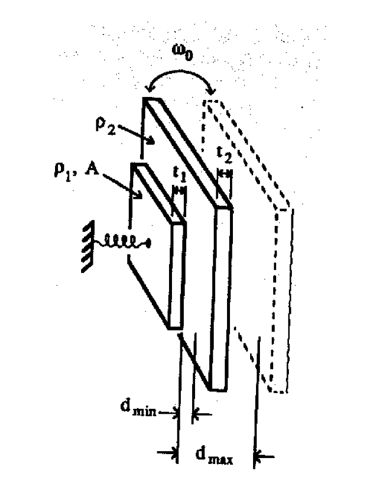
Figure 1: Configuration of the prototype experiment discussed in the text.

The main advantage of a configuration of the type of that of Fig.1 is that it is a null gravity experiment: i.e. gravity is constant between the two parallel plates. In the Fourier transformed domain I am thus lead to a signal which is different from zero only for deviations from gravity which, as usual, are parametrized by a Yukawa type potential

$$V(r)=-G_{N}^{(4)}\alpha\int_{V_{d}}d^{3}x{e^{-{r\over\lambda}}\over r}$$ (50)

which expresses the interaction of an atom of the generator plate (of area $A$, thickness $t_{1}$, density $\rho_{1}$) with the detector plate which is taken to have geometrical dimensions such that its area is much bigger than $A$. Integrating over the generator plate and taking the derivative with respect to the distance between the two parallel plates, I find the force

$$F_{Y}=-2\pi\alpha G_{N}^{(4)}\rho_{1}\rho_{2}\lambda^{2}Ae^{-{d(t)\over\lambda}}(1-e^{-{t_{1}\over\lambda}})(1-e^{-{t_{2}\over\lambda}}),$$ (51)

where $d(t)=\bar{d}+d_{0}\sin\omega_{0}t$ is the distance between the two plates with $d_{0}=(d_{max}-d_{min})/2$ and $\bar{d}=(d_{max}+d_{min})/2$. Fourier transforming (51) leads to

$$\widetilde{F}_{Y}=-2\pi\alpha G_{N}^{(4)}\rho_{1}\rho_{2}A\lambda^{2}I_{1}({d_{0}\over\lambda})e^{-{\bar{d}\over\lambda}}(1-e^{-{t_{1}\over\lambda}})(1-e^{-{t_{2}\over\lambda}}),$$ (52)

where $I_{1}$ is a Bessel function. To obtain (52) I have used the fact that only the oscillator first resonant mode is relevant for our discussion. An estimate of the noise is given by

$$F_{noise}=\sqrt{kTm\omega_{0}\over Q\tau},$$ (53)

where m is the mass of the detector, k is the Boltzmann constant, T the temperature at which the experiment is performed, Q is the detector’s quality factor and $\tau$ the integration time. Plugging into (53) typical values for the quantities involved, I get $F_{noise}\approx 10^{-10}$ dyne. The ratio between (52) and (53) gives the signal to noise ratio, SNR. A proposed experiment along these lines has been described in [12].

Let me now examine what are the main sources of noise that have to be monitored in such an experiment:

• Casimir type forces

• Surface type forces

Fourier transforming the Casimir force between two parallel plates, I get

$$\widetilde{F}_{Casimir}=-{\pi^{2}\hbar cA\over 280}{(d_{0}^{3}+4d_{0}^{2}\bar{d})\over(d_{0}^{2}+\bar{d}^{2})^{7/2}}$$ (54)

For values typical of these experiments (probing gravity at the mm scale) $\widetilde{F}_{Casimir}\approx 10^{-12}$ dyne that is a value which is a couple of order of magnitude smaller than our noise. Consequently I do not have to worry about corrections to (54) coming from lack of parallelism between the plates, the temperature being different from zero, the materials being not perfect metals or the two plates being not at rest.

Let me come now to the second source of noise which I have denoted surface type forces because they are generated by the superficial properties of the two plates. It is in fact well known that if I put in front of each other two materials I can measure in the space between the two an electric field of the order of the tens of millivolt. This field is generated by patches of charges on the surface of the materials which, in first istance I attribute to impurities on the parallel two surfaces. An estimate of the force generated is given by

$$F_{electric}={1\over 4\pi}{(\Delta V)^{2}A\over(\bar{d}+d_{0}\sin\omega_{0}t)^{2}}\approx 10^{-10}{A\over(\bar{d}+d_{0}\sin\omega_{0}t)^{2}}{\rm dyne}.$$ (55)

The strength of $F_{electric}$ is such that it could overcome the signal from the Yukawa potential. From the experimental point of view this force is dealt with by connecting the two material to earth and among them or giving a bias current to balance for the phenomena. Giving the importance of the consequences of the presence of $F_{electric}$ it is then time to better understand the physics of the problem. If the material of which the two plates are made are different metals, then the electric field originates from the difference of the Fermi levels between the two. But even if the materials are the same the effect is still there, due to the fact that the metals are not monocrystals. It is anyway possible two coat the two plates with a thin layer of monocrystal material. Few angström are sufficient to change the superficial properties. In my opinion this is the most elegant way to cope with this problem.

In conclusion, in this chapter I have shown that performing experiments of gravity at the mm scale is possible given our understanding of the possible noise sources. I hope that very soon we will have experimental data to discuss.

References

- [1] C.M. Will, Theory and Experiment in Gravitational Physics (Cambridge University Press, Cambridge, 1993).
- [2] M. Bianchi, M. Brunetti, E. Coccia, F. Fucito, and J.A. Lobo, Phys. Rev. D 57, 4525 (1998).
- [3] J.A. Lobo, Phys. Rev. D 52, 591 (1995).
- [4] R.V. Wagoner and H.J. Paik in Proc. of the Int. Symposium on Experimental Gravitation (Accademia Nazionale dei Lincei, Rome, 1977).
- [5] E. Coccia, V. Fafone, G. Frossati, J. A. Lobo and J. A. Ortega, Phys. Rev. D 57, 2051 (1998).
- [6] F.J. Raab (LIGO team), in E. Coccia, G.Pizzella, F.Ronga (eds.), Gravitational Wave Experiments, Proceedings of the First Edoardo Amaldi Conference, Frascati 1994 (World Scientific, Singapore, 1995).
- [7] A. Giazotto et al. (VIRGO collaboration), in E. Coccia, G.Pizzella, F.Ronga (eds.), Gravitational Wave Experiments, Proceedings of the First Edoardo Amaldi Conference, Frascati 1994 (World Scientific, Singapore, 1995).
- [8] P. Jordan, Z. Phys., 157, 112 (1959).
- [9] C. Brans and R. H. Dicke, Phys. Rev. 124, 925 (1961).
- [10] M. Brunetti, E. Coccia, V. Fafone and F. Fucito, Phys. Rev. D 59, 044027 (1999).
- [11] E. Coccia, F. Fucito, J. A. Lobo and M. Salvino to appear in Phys. Rev. D62, 044019 (2000).
- [12] J. C. Long, H. W. Chan and J. C. Price, Nucl. Phys. B539 (1999) 23.
- [13] A.E.H. Love, A Treatise on the Mathematical Theory of Elasticity, Dover 1944.
- [14] L. D. Landau and E. M. Lifshitz, Theory of Elasticity, Pergamon 1970.
- [15] M. Abramowitz and I.A. Stegun, Handbook of Mathematical Functions, Dover 1972.
- [16] M. Bianchi, E. Coccia, C. N. Colacino, V. Fafone, and F. Fucito, Class. and Quantum Grav. 13, 2865 (1996).
- [17] S. Weinberg, Gravitation and Cosmology, Wiley & sons, New York 1972.
- [18] E. Coccia and V. Fafone, Phys. Lett. A 213, 16 (1996).
- [19] M. Shibata, K. Nakao and T. Nakamura, Phys. Rev. D 50, 7304 (1994); M. Saijo, H. Shinkai and K. Maeda, Phys. Rev. D 56, 785 (1997).
- [20] N. Arkani-Hamed, S. Dimopoulos, G. Dvali, Phys. Lett. B429 263 (1998).
- [21] I. Antoniadis, N. Arkani-Hamed, S. Dimopoulos and G. Dvali, Phys. Lett. B436 257 (1998).
- [22] I. Antoniadis, S. Dimopoulos and G. Dvali, Nucl. Phys. B516 70 (1998).
- [23] E. Fischbach and C. Talmadge, The Search for Non-Newtonian Gravity (AIP Press/Springer-Verlach, New York 1999).