Gravitational waves from extreme mass ratio inspirals: Challenges in mapping the spacetime of massive, compact objects

Abstract

In its final year of inspiral, a stellar mass ($1-10M_{\odot}$) body orbits a massive ($10^{5}-10^{7}M_{\odot}$) compact object about $10^{5}$ times, spiralling from several Schwarzschild radii to the last stable orbit. These orbits are deep in the massive object’s strong field, so the gravitational waves that they produce probe the strong field nature of the object’s spacetime. Measuring these waves can, in principle, be used to “map” this spacetime, allowing observers to test whether the object is a black hole or something more exotic. Such measurements will require a good theoretical understanding of wave generation during inspiral. In this article, I discuss the major theoretical challenges standing in the way of building such maps from gravitational-wave observations, as well as recent progress in producing extreme mass ratio inspirals and waveforms.

Chandrasekhar has described black holes as “the most perfect macroscopic objects there are in the universe” [1]. This description refers to their simplicity, depending (in astrophysical contexts) solely on the mass and spin of the hole. This dependence, in turn, follows from the black hole uniqueness theorems [2, 3, 4, 5, 6], which guarantee that all of the other “hairs” will radiate away during the hole’s formation. If general relativity correctly describes gravity, then the massive compact objects at the centers of most galaxies are probably described exactly by the Kerr rotating black hole metric. In principle, this description can be tested using LISA [7]: gravitational-wave observations of “small” ($1-10\,M_{\odot}$) bodies spiralling into “large” ($10^{5}-10^{7}\,M_{\odot}$) compact objects can be used to map the spacetime of the large compact object, testing whether it is a Kerr black hole or some other exotic object. In this article, I discuss the theoretical challenges that must be met before such maps can be constructed, as well as recent progress.

Fintan Ryan [8] first showed that a body’s spacetime can be mapped with gravitational waves. The spacetime of a massive object arises from its multipole moment structure. These multipole moments come in two varieties, mass ($M_{l}$) and current ($S_{l}$). If $\rho(\vec{r})$ is the mass density at position $\vec{r}$, and $\vec{v}(\vec{r})$ is the fluid velocity at $\vec{r}$, then these multipoles are roughly

$$M_{l}\simeq\int\rmd^{3}r\,r^{l}\rho({\vec{r}})\,,\qquad S_{l}\simeq\int\rmd^{3}r\,r^{l-1}\left[{\vec{r}}\times{\vec{v}(\vec{r})}\rho(\vec{r})\right]$$ (1)

For a black hole, the mass and current multipole moments take a far simpler form:

$$M^{\rm BH}_{l}+\rmi S^{\rm BH}_{l}=M(\rmi a)^{l}$$ (2)

Because these moments directly determine the spacetime, the orbits of and radiation emitted by a small body moving in this spacetime are strongly influenced by the massive object’s multipoles. Measuring the radiation allows one (in principle) to measure the multipolar structure of the massive object.

Much work remains before it will be possible to measure an exotic body’s multipole moments in practice. In particular, techniques must be developed to solve the wave equation for gravitational radiation from orbits of exotic objects. This is not a terribly difficult matter for black hole spacetimes — following Teukolsky’s 1972 discovery [9] that the wave equation for radiation propagating in Kerr spacetimes is separable, an array of calculational technology has been developed for studying the generation and propagation of such radiation (see, e.g., [10] for review and discussion). Very little work has been done for radiation generated in and propagating through the spacetime of more exotic objects: Ryan [11] has examined the scalar waves produced by highly constrained orbits (circular and equatorial) of objects with arbitrary multipole moments. We are a long way from understanding the waveforms created by orbits of non-black hole objects. Such an understanding will be needed — at least to some degree — in order to probe the multipole character of massive compact bodies.

For now, we simplify the problem by focusing upon waves generated when the massive object is a black hole. Of greatest interest is understanding the waves emitted as a small, spinning body spirals into a massive Kerr black hole. Neglecting radiation reaction, the motion of such a body is governed by the Papapetrou equations [12]:

$${Dp^{\mu}\over D\tau} =-{1\over 2}R^{\mu}_{\nu\rho\sigma}v^{\nu}S^{\rho\sigma}$$

$${DS^{\mu\nu}\over D\tau} =p^{\mu}v^{\nu}-p^{\nu}v^{\mu}$$ (3)

In these equations, $D/D\tau$ denotes a covariant derivative along the small body’s trajectory, $R^{\mu}_{\nu\rho\sigma}$ is the Riemann curvature tensor of the background spacetime, $S^{\mu\nu}$ is a tensor related to the spin of the body, $v^{\mu}=dz^{\mu}/d\tau$ where $z^{\mu}(\tau)$ is the coordinate worldline of the body, and $p^{\mu}$ is a generalization of the body’s 4-momentum that incorporates spin. These equations show that as the small body orbits, its spin couples to the curvature of the massive black hole. In the weak field, this coupling is known to lead to precessional effects which modulate the phase and amplitude of the gravitational waveform [13]. In the strong field, the coupling might become extremely important. It is likely that, at least for certain parameter values, the orbital character will become chaotic. Janna Levin [14] has shown that integrating the second post-Newtonian equivalents of Equation (3) leads to chaotic motion: orbits with similar initial conditions evolve to vastly different configurations. This could make data analysis extremely difficult — matched filtering, for example, would require an enormous number of templates in order to cover all possible inspirals. When radiation reaction is included, the effects of chaos in Levin’s work become less extreme: she focused upon sources of interest to ground-based detectors, and the number of orbits visible to those detectors is not very large. With LISA, though, we expect to see around $10^{5}$ orbits. Chaotic evolution could lead to a dramatic divergence of outcomes from similar initial conditions, rendering data analysis practically impossible. Detailed studies of these orbits with parameters relevant to LISA are urgently needed.

Since spin opens an as-yet-poorly-understood can of worms, we will ignore it for now, treating the small body as a point perturbation to the Kerr spacetime. At zeroth order, this small body moves on a Kerr geodesic. For such orbits, a relatively mature radiation reaction formalism (see, e.g., [15] and references therein) has been developed that finds the first order radiative corrections to this motion, allowing one to compute the trajectory that the body follows as it spirals into the black hole, and the waveforms that it generates. This formalism uses the zeroth order geodesic motion as a source for the first order corrections. As such, it assumes that the inspiral is adiabatic: the timescale for radiation reaction to change the orbit’s characteristics is much smaller than the orbit’s dynamical timescale.

For the most interesting orbits — eccentric, inclined orbits in the strong field of rotating black holes — it is not clear at the present time if this adiabatic approximation is reasonable. It is somewhat difficult to define the orbit’s dynamical timescale in this interesting case. The issue is that there are three physically meaningful timescales: the time $T_{\phi}$ for the body to cover $0\leq\phi\leq 2\pi$; the time $T_{r}$ for the body to move from $r_{\rm max}$ to $r_{\rm min}$ and back; and the time $T_{\theta}$ for the body to move from its highest latitude $\theta_{\rm min}$ to its lowest $\theta_{\rm max}$ and back. These timescales generically are rather different. When the orbit is constrained (eccentric but equatorial, or inclined but circular) only two of these timescales are non-zero. One can analyze the orbit in a frame that rotates at frequency $\Omega=2\pi/T_{\phi}$, cancelling out the $\phi$ motion. It is then simple to define the orbit’s dynamical timescale: it is $T_{r}$ (for eccentric, equatorial orbits) or $T_{\theta}$ (for inclined, circular orbits) (see [15] for more detail).

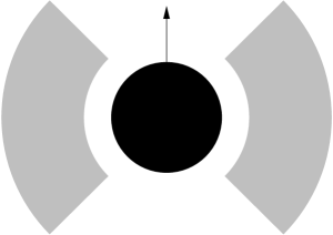
Figure 1: A slice of the orbital torus. The dark circle is the central Kerr black hole; the grey region is the volume which is filled by the orbiting body. The full torus is given by rotating this figure about the spin axis (indicated by the arrow).

When the motion is not constrained, this trick does not work. To understand the behavior of the orbit for the general case, consider Figure 1. This figure shows a 2-dimensional slice of the volume that is filled by a small body as it orbits the black hole: as it moves from $r_{\rm min}$ to $r_{\rm max}$ it simultaneously moves between $\theta_{\rm min}$ and $\theta_{\rm max}$. Rotating this figure about the black hole’s spin axis, we see that the orbit ergodically fills a torus in the spacetime near the hole’s horizon. For adiabaticity to be a good approximation, the orbiting body must come “close” to every point in this volume. (The meaning of “close” is of course rather ambiguous. “Close enough” depends upon the accuracy that one requires, which in turn depends upon how well one needs to know the phase of the waveform.) An important problem is to determine how long it takes for an orbiting body to come “close enough” to all points in this volume for parameters that are of interest to LISA observations (strong field, large black hole spin, high eccentricity, and arbitary inclination angle). If this time turns out to be larger than the radiation reaction timescale then further studies of these waveforms will require radiation reaction forces that do not rely on adiabaticity [16, 17, 18, 19, 20, 21, 22]. The phase evolution of waveforms that one constructs in these cases may have a strong dependence on the orbiting body’s initial conditions — they may be “effectively chaotic” in the words of Schutz [23].

Even if it turns out that the issue of adiabaticity is not a serious problem, there is still an important challenge that must be faced in order to evolve generic Kerr orbits. Such orbits are characterized by three conserved quantities: the energy $E$, the $z$-component of angular momentum $L_{z}$, and the Carter constant $Q$. For Schwarzschild black holes, $Q$ is just $L_{x}^{2}+L_{y}^{2}$, the other angular momentum components. Interpretation of the Carter constant becomes less clear as $a$ increases (the geometry becomes oblate, confusing the meaning of $x$, $y$, and $z$, and frame dragging entangles the $t$ and $\phi$ coordinates), but it is useful to regard it essentially as the “rest” of the small body’s angular momentum. At present, the most mature computational formalisms (such as that described in [15]) cannot evolve $Q$. These formalisms work by a method of “flux-balancing”: from the flux of gravitational waves going to infinity and down the hole’s event horizon, one can easily deduce the change in $E$ and $L_{z}$ because of gravitational-wave emission. One cannot easily deduce the change in $Q$, except in special cases (for eccentric equatorial orbits, $Q=0$ at all times; for inclined, circular orbits theorems which prove that the orbit adiabatically remains circular [24, 25, 26] allow one to express $dQ/dt$ as a function of $dE/dt$ and $dL_{z}/dt$). Although clever methods may make it possible to evolve $Q$ just by examining the radiation flux at infinity and at the horizon (see Wolfgang Tichy’s contribution to these proceedings), it may turn out that a local radiation reaction force will be needed.

At this point, the current unsolved or poorly understood issues have narrowed the class of sources that are well understood rather severely. Current computational technology is limited to understanding the adiabatic evolution of spinless bodies on constrained orbits — either eccentric equatorial orbits or inclined circular orbits. For the remainder of this article, I will focus on circular inclined orbits, as described in [15]; Daniel Kennefick and Kostas Glampedakis are developing an analysis of eccentric equatorial orbits using a similar formalism.

Figure 2: Inspiral from $r=4M$ to the last stable orbit (indicated by the dotted line). The massive black hole has $M=10^{6}\,M_{\odot}$ and $a=0.998M$; the small body has $\mu=1\,M_{\odot}$. The left-hand panel shows the inspiral including both flux to infinity and flux down the horizon; the right-hand panel includes only flux to infinity. Notice that the horizon flux typically slows the inspiral.

Using the formalism and code described in [15], I have studied the inspirals and associated gravitational waveforms for a large number of strong-field initial conditions. The results for $a=0.998M$ are shown in the left-hand panel of Figure 2. This figure shows the inclination angle $\iota$ of the orbit as the small body spirals from $r=4M$ to the last stable orbit (LSO); it also shows the number of days that pass along this sequence. In all cases the trajectory is nearly flat — the inclination does not change very much as the small body inspirals. The inclination evolution is even flatter at smaller values of $a$ [27]. Curt Cutler has suggested that this might be used as the basis of an approximate scheme for evolving the Carter constant for generic orbits: if it is true in general that the inclination angle does not change very strongly, then it might be a reasonable approximation to set the change to zero. This condition would constrain the evolution of $Q$. Cutler’s approximation may be useful for developing approximate waveforms for the study of data analysis tools.

Turn now to the right-hand panel of Figure 2. This panel is identical to the left-hand panel except that the flux of radiation down the massive black hole’s event horizon has been ignored in constructing the inspiral trajectory. Although the shape does not change very much, the time it takes to inspiral is significantly smaller: the horizon flux slows the inspiral by several weeks at low inclination angle. This is a significant effect — change of the inspiral time by such a large amount should be easily measurable. At first glance, it is also rather counterintuitive: one expects the hole’s event horizon to be a sink of energy, so the inspiral would speed up as radiation flows into the hole. This simple picture is wrong when the hole rotates. A more accurate picture can be developed by considering the tidal coupling of the black hole to the inspiralling body. The tidal field of the small body will distort the hole, raising “bulges” in the event horizon [28]. These bulges exert a torque back on the small body. When the hole is rapidly spinning, the bulges are dragged ahead of the orbiting body so that this torque tends to increase the orbiting particle’s energy. This partially offsets the energy that is lost from radiation to infinity, slowing the inspiral.

One of the major goals of this analysis is to produce gravitational waveforms. Using the inspiral trajectories shown in the left-hand panel of Figure 2, I have developed the associated gravitational waveforms:

$$h_{+}(t)-\rmi h_{\times}(t)={\mu\over D}\sum_{l=2}^{\infty}\sum_{m=-l}^{l}\sum_{k=-\infty}^{\infty}{Z_{lmk}\left[r(t),\iota(t)\right]\over\omega_{mk}^{2}}\,S_{lm}(\vartheta)\,\rme^{\left[\rmi(m\varphi-\omega_{mk}t)\right]}$$ (4)

Here, $\mu$ is the mass of the small body, $D$ is the luminosity distance to the source, $[r(t),\iota(t)]$ is the inspiral trajectory, $Z_{lmk}[r,\iota]$ is a complex amplitude computed with the Teukolsky equation, $\omega_{mk}=m\Omega_{\phi}+k\Omega_{\theta}$, $S_{lm}$ is a spin-weighted spheroidal harmonic, and $(\vartheta,\varphi)$ is the angular position of the observer relative to the spin axis. Perhaps the most effective demonstration of the characteristics of these waveforms is given by converting the functions $h_{+}(t)$ and $h_{\times}(t)$ into sounds; the reader is invited to visit the URL given in [29] and listen to the sounds available there. Some of the features one can hear in these waveforms are rather surprising. For instance, in several cases, the wave chirps down as well as chirps up: a portion of the sound has decreasing frequency. Despite the many simplifications that were imposed in order to compute these waves, they have a rather complex and ornate character.

As the challenges discussed earlier are surmounted we will be able to develop waveforms that incorporate even more structure and complexity. The surprising features that were found for simple circular orbits will doubtless be joined by more surprises, increasing the complexity of the waveforms. This complexity will make it difficult to detect and analyse the waves in LISA data, but is indicative of how much can be learned from their observation.

I would like to thank Pat Brady, Curt Cutler, Mike Hartl, Janna Levin, Lee Lindblom, Sterl Phinney, Tom Prince and Kip Thorne for many useful discussions and support. This research was supported by NSF Grants AST-9731698 and AST-9618537 and NASA Grants NAG5-6840 and NAG5-7034.

References

References

- [1] Chandrasekhar S 1983, The Mathematical Theory of Black Holes (New York: Oxford University Press) p 1
- [2] Israel W 1967 Phys. Rev.164 1776
- [3] Carter B 1971 Phys. Rev. Lett.26 331
- [4] Robinson D C 1975 Phys. Rev. Lett.34 905
- [5] Price R H 1972 Phys. Rev.D 5 2419
- [6] Price R H 1972 Phys. Rev.D 5 2439
- [7] Danzmann K et al. 1998 LISA: Proposal for a Laser-Interferometric Gravitational Wave Detector in Space Max-Planck-Institut für Quantenoptik Report MPQ 233, Garching, Germany
- [8] Ryan F D 1997 Phys. Rev.D 56 1845
- [9] Teukolsky S A 1973 Astrophys. J. 185 635
- [10] Hughes S A 2000 Phys. Rev.D 62 044029
- [11] Ryan F D 1997 Phys. Rev.D 56 7732
- [12] Dixon W G 1979 Isolated Gravitating Systems in General Relativity ed J Ehlers (Amsterdam: North-Holland) p 156
- [13] Apostolatos T A, Cutler C, Sussman G J and Thorne K S 1994 Phys. Rev.D 49 6274
- [14] Levin J 2000 Phys. Rev. Lett.84 3515
- [15] Hughes S A 2000 Phys. Rev.D 61 084004
- [16] Quinn T C and Wald R M 1997 Phys. Rev.D 56 3381 (1997)
- [17] Mino Y, Sasaki M and Tanaka T 1997 Phys. Rev.D 55 3457
- [18] Wiseman A G 2000 Phys. Rev.D 61 084014
- [19] Ori A 1997 Phys. Rev.D 55 3444
- [20] Barack L and Ori A 2000 Phys. Rev.D 61 061502
- [21] Burko L M 2000 Phys. Rev. Lett.84 4529
- [22] Lousto C 2000 Phys. Rev. Lett.84 5251
- [23] Schutz B 1998 private communication
- [24] Kennefick D and Ori A 1996 Phys. Rev.D 53 4319
- [25] Ryan F D 1996 Phys. Rev.D 53 3064
- [26] Mino Y 1996 unpublished Ph.D. thesis (Kyoto University)
- [27] Hughes S A 2000 in preparation
- [28] Hartle J 1974 Phys. Rev.D 9 2749
- [29] Audio representations of these inspiral waveforms in Sun .au format can be downloaded from http://www.tapir.caltech.edu/~hughes/Research/RRKerr/wave_spec.html