Scattering of particles by neutron stars: Time-evolutions for axial perturbations

Abstract

The excitation of the axial quasi-normal modes of a relativistic star by scattered particles is studied by evolving the time dependent perturbation equations. This work is the first step towards the understanding of more complicated perturbative processes, like the capture or the scattering of particles by rotating stars. In addition, it may serve as a test for the results of the full nonlinear evolution of binary systems.

I Introduction

The gravitational interaction of massive bodies in general relativity is associated to the emission of gravitational signals, the features of which depend on the nature of the interacting bodies and on the characteristics of their orbits. To be studied in detail, very energetic processes like the coalescence of binary systems need the complex machinery of the fully non linear theory of gravity coupled to hydrodynamics; this challenging task has been undertaken by several scientific groups in the world [1],[2],[3], [4]. Waiting for the outcome of these simulations, approximation methods which allow to get preliminary information on these processes are extremely useful. An example of the way in which approximate methods shed light on much more complex phenomena, is the capture of test particles by a black hole (see ref. [5] for a review). On the assumption that the infalling mass is much smaller than the black hole mass, so that its effect can be treated as a perturbation of the black hole geometry, it was shown that the gravitational signal emitted in this process exhibits a ringing tail due to the excitation of the quasi normal modes of the perturbed black hole. Years later, a fully relativistic numerical simulation of the gravitational collapse of a massive star to a black hole [6] showed that the signal emitted in this process also exhibits an exponentially damped sinusoidal tail. The experience matured in black hole perturbations suggested that this tail appears because the newly born black hole radiates its residual mechanical energy oscillating in its quasi-normal modes.

A further element of interest in the use of perturbation theory is that the results will serve as a test for fully nonlinear calculations [7]. For instance, the nonlinear evolution of the head on collision of two black holes [8] has proved to be in excellent agreement with the results obtained via a perturbative approach.

The gravitational signals emitted by massive particles orbiting around rotating and non-rotating black holes have been extensively investigated [5], and more recently this study has been extended to the signals emitted when small masses in open or circular orbit, interact with a compact non rotating star [9]-[13]. By a direct integration of the equations describing the perturbation of the star, it has been shown that both its fluid modes and the spacetime modes can in principle be excited, if the scattered mass is allowed to get sufficiently close to the compact star. These results have been obtained by Fourier transforming the perturbation equations, and solving the associated boundary value problem, with the condition that the solution is regular at the center of the star, and reduces to a pure outgoing wave at radial infinity.

This approach is very powerful when masses are in open or closed orbits around a non rotating star; however, it cannot be applied if the mass falls onto the star, due to the lack of information on the interaction between the particle and the stellar fluid after the impact. To investigate this kind of problems, a time evolution approach seems more appropriate than the analysis in the frequency domain, since it allows to compute the emitted signal at least up to when the particle touches the surface of the star. It appears promising also to describe the perturbations of rotating stars excited by small masses. Indeed, in that case the coupling between the axial and polar perturbations which arises as a consequence of the dragging of inertial frames ([14], [15]), leads to a set of equations that are not simply reducible to wave equations as in the case of a non rotating star. Moreover, the time evolution approach has recently been used in the literature to study the scattering of wave packets by non rotating relativistic stars, ([16], [17], [18], [19]), where it has been shown to correctly reproduce the spectra of axial and polar perturbations, in a perturbative study of colliding neutron stars [20] (close limit), and to provide proper initial data for stellar perturbations [21].

These considerations motivate the work done in this paper: we develop a scheme for the numerical evolution of stellar perturbations excited by a scattered mass. In order to allow a direct comparison with previously obtained results, we integrate the equations describing the axial perturbations of a homogeneous star with increasing compactness, for different values of the orbital parameters of the scattered mass, and we choose the same stellar and orbital parameters as in ref. [11], where the axial equations were integrated in the frequency domain.

It should be mentioned that the time-evolution equations do not suffer of the annoying problem of the divergence of the source term when the particle transits through the turning point, which causes some difficulties in the integration of the Regge-Wheeler and of the Zerilli equations in the frequency domain.

The plan of the paper is the following. In section II we shall briefly review the time-dependent version of the equations of the axial perturbations. In section III we shall present the results of the numerical integration. Our energy spectra will be compared with those found in [11] and [12] and the differences will be discussed. In the Appendix we shall show that the low-frequency part of the spectrum can be traced back to the bremsstrahlung radiation emitted by the scattered mass.

II The equations describing the perturbed spacetime

In order to describe the non axisymmetric perturbations of a star induced by a scattered particle, we expand the perturbed metric in tensor spherical harmonics, and choose the Regge-Wheeler gauge. The perturbed line element has the form:

$$ds^{2} = e^{2\nu}dt^{2}-e^{2\mu_{2}}dr^{2}-r^{2}d\vartheta^{2}-r^{2}\sin^{2}\vartheta d\varphi^{2}$$ (1)

$$+ 2\sin\theta{\partial Y_{\ell m}\over\partial\theta}\left[h^{0}_{\ell m}(t,r)dtd\varphi+h^{1}_{\ell m}(t,r)drd\varphi\right]$$ (2)

$$- \frac{2}{\sin\vartheta}\frac{\partial Y_{\ell m}}{\partial\varphi}\left[h^{0}_{\ell m}(t,r)dtd\vartheta+h^{1}_{\ell m}(t,r)drd\vartheta\right]$$ (3)

We consider the perturbations of a non rotating star with uniform energy density $\epsilon=$const [22]. It should be reminded that homogeneous stars can exist only if their radius $R$ exceeds 9/8 times the Schwarzschild radius, or $R/M>2.25$ (Buchdahl limit). The source of the perturbed Einstein equations is given by the stress-energy tensor of the particle moving along a geodesic of the Schwarzschild spacetime  $(T(t),R(t),\Theta(t),\Phi(t))$  :

$$T^{\mu\nu}_{(p)}=m_{0}\frac{dT(t)}{d\tau}\frac{dz^{\mu}}{dt}\frac{dz^{\nu}}{dt}\frac{\delta(r-R(t))}{r^{2}}\delta(\Omega-\Omega(t)).$$ (4)

With this source, and assuming that the particle moves on the equatorial plane $\Theta=\frac{\pi}{2}$, the axial perturbations can be shown to be described by the following equation ([22], [11])

$$\frac{d^{2}Z_{\ell m}(t,r)}{dt^{2}} - \frac{d^{2}Z_{\ell m}(t,r)}{dr_{*}^{2}}+V_{\ell}(r)Z_{\ell m}(t,r)$$ (5)

$$= -16\pi\imath e^{2\nu}\left[r\left(e^{2\nu}D_{\ell m}\right)_{,r}-e^{2\nu}Q_{\ell m}\right]$$ (6)

where

$$Z_{\ell m}(t,r)=\frac{e^{\nu-\mu_{2}}}{r}h_{1}(t,r)$$ (7)

is a gauge invariant quantity, $r_{*}$ is the tortoise coordinate and

$$V_{\ell}=(e^{2\nu}/r^{3})\left[\ell(\ell+1)r+r^{3}(\epsilon-p)-6m(r)\right]$$ (8)

is the potential, which reduces to the Regge-Wheeler potential outside the star, where pressure and density vanish ($p=\epsilon=0$). The two functions $D_{\ell m}$ and $Q_{\ell m}$, related to the particle’s motion, have the following form:

$$D_{\ell m}(r,t) = -\frac{\mu m}{\ell(\ell+1)(\ell-1)(\ell+2)}~{}\frac{L^{2}_{z}}{E}~{}\frac{e^{2\nu}}{r^{4}}~{}\delta(r-R(t))\cdot Y^{\ast}_{\ell m,\vartheta}\left|{}_{\Theta=\frac{\pi}{2},\Phi(t)}\right.$$ (9)

$$Q_{\ell m}(r,t) = -\frac{\imath\mu e^{-2\nu}}{\ell(\ell+1)}\frac{L_{z}}{r^{3}}\frac{dR}{dt}~{}\delta(r-R(t))\cdot{Y^{\ast}_{\ell m,\vartheta}}\left|{}_{\Theta=\frac{\pi}{2},\Phi(t)}\right.$$ (10)

where $\mu$ is the mass of the particle.

The one-sided energy spectrum of gravitational waves at infinity will be calculated from the following relation

$${dE\over d\omega}={1\over 16\pi^{2}}\sum^{\infty}_{\ell=2}\sum^{\ell}_{m=-\ell}(\ell-1)\ell(\ell+1)(\ell+2)|Z_{\ell m}(\omega)|^{2},$$ (11)

where  $Z_{\ell m}(\omega)$  is the Fourier transform of the wavefunction  $Z_{\ell m}(t,r),$  evaluated at radial infinity. For the axial perturbation, we have to deal only with multipoles with $m=l-1,l-3,\dots$ since the multipoles with $m=l,l-2,\dots$ correspond to polar perturbations. For the purpose of this paper we will present results only for $l=2$ and $m=1$.

III Numerical method and results.

The numerical procedure we follow to calculate the energy spectrum can be described by the following steps

• For a specific stellar model and for a given set of values of the energy and of the angular momentum of the particle, $(E,L_{z})$, we calculate the geodesics i.e. the position of the particle, for a discrete number of time steps from $r\to\infty$ up to $r=r_{t}$ ($r_{t}$ is the turning point of the given open trajectory).

• For the specific geodesic, we estimate the source term of (5) for each time and spatial grid point. Since there is no back reaction this calculation is done only once at the beginning.

• According to equations (9)-(10) the position of the particle at each time step is represented by a delta function, that we approximate by a narrow Gaussian function

  $$\delta(r-R(t))\approx{\alpha\over{\sqrt{\pi}}}e^{-\alpha^{2}(r-R(t))^{2}}$$ (12)

  (this approximation has been also used in [13]). The code has been tested for various values of $\alpha$ in order to check the way in which the width of the Gaussian affects the results.

• Finally, eq. (5) is evolved using a second order finite-difference scheme. The results have been tested for various grid sizes in order to achieve the required accuracy.

In Figure 1 we plot two waveforms corresponding to a particle with orbital parameters $(E,L_{z})=(2.38\mu,12\mu M)$ scattered by two homogenous stars, one with compactness $R/M=2.26$ and the other with $R/M=2.30$. The initial part of the signal is similar in both cases, since it is due mainly to the accelerated particle, whereas the subsequent oscillations have different frequencies and damping times since they are due to the excitation of the axial modes of the two stars. The energy spectrum of the above signals, calculated via eq. (11), is shown in Figure 2. On the same figure, we mark the location of the real part of the frequency of the axial quasi-normal modes of the two stars, as computed in [23] by solving the homogeneous equation as a boundary value problem. It comes out that the lowest trapped modes, that have much longer damping times, do not seem to be excited, whereas the higest w-modes are clearly excited in both cases. In Figure 3 we show the energy spectrum for a less energetic particle $(E,L_{z})=(1.01\mu,4.5\mu M)$; here one can easily identify the peaks corresponding to the excitation of the w-modes, but the bulk of the emitted energy is due to the quadrupole emission of the accelerated particle. This continues to be true if the central star is less relativistic. These results suggest that in order to have a significant excitation of the stellar axial modes one needs both the periastron of the scattering orbit to be as close as possible to the stellar surface, and the star to be of high compactness. The above features agree with the results of ref. [10], where the axial and polar emission for particles scattered by a compact polytropic star was studied in the frequency domain, and with those presented in [13], where the polar mode excitation by scattered particles has been studied with a time-evolution approach.

Our results also qualitatively agree with those of ref. [11], as a comparison of our figure 2 and 3 with their figures 5, 6 or 8 clearly show. However, there is a difference of a factor $\sim 2\pi$ in the energy spectra, which is probably due to a different normalization. More relevant is the difference we find in the energy spectra at low frequency: we observe some peaks that do not appear either in the spectra of ref. [11], or in those presented in ref. [12]. Since this same feature also appeared in previous works ([10] and [13]), we have investigated the low frequency behaviour in some more detail. We have computed the energy spectrum emitted by the same scattered particles in a semirelativistic approximation, by assuming that the particles move along a geodesic of the background geometry, but radiate as if they were in flat spacetime, according to the quadrupole formula. The energy spectra estimated by this procedure are shown in Figure 4 for the star with $R/M=2.26$ and for $(E,L_{z})=(2.38\mu,12\mu M)$ and $(E,L_{z})=(1.01\mu,4.5\mu M)$ (details of this calculation are given in the Appendix). We find low frequency peaks which correspond to those in figures 2 and 3; this indicates that the low frequency part of the energy spectrum is “shaped” by the bremsstrahlung radiation emitted by the accelerated particle. It should be mentioned that one should not expect an exact coincidence between the results of the semirelativistic approximation and of the relativistic approach, especially when the orbit of the scattered particle is very relativistic. However, the two approaches must tend to the same limit when the particle moves on less relativistic orbit, and we have checked that this is indeed the case.

As a concluding remak, we would like to point out that the calculations presented in this paper prove that the numerical evolution of the time dependent perturbation equations is a fast and accurate way to study scattering processes occurring in the vicinity of a neutron stars; they allow to obtain detailed information either on the amount of energy emitted at low frequency, which can be traced back to the quadrupole emission, and on the excitation of the neutron star quasi-normal modes. In a future work we plan to extend the present investigation to the study of the excitations of the stellar modes of rotating stars. There, the coupling of the axial and polar perturbations makes the whole process more complicated and the numerical evolution of the perturbation equations appears a promising approach.

APPENDIX: The quadrupole emission of the scattered mass

In order to understand what is the contribution of the gravitational radiation emitted by the accelerated particle to the total energy spectrum, we have used a semi-relativistic approximation introduced in 1971 [24], which assumes that the particle moves along a geodesic of the curved spacetime, but radiates as if it were in flat spacetime. On this assumption, using the quadrupole formula, we have computed the TT-components of the gravitational wave emitted by the scattered mass. As usual, the reduced quadrupole moment is

$$Q_{kl}=\mu\left(X^{k}X^{l}-\frac{1}{3}\delta^{k}_{l}\left|{\mathbf{X}}\right|^{2}\right),$$ (13)

where the two-dimensional vector  ${\mathbf{X}}$  is the position of the particle along its trajectory in the equatorial plane ${\mathbf{X}}=\left(R(t)\cos\Phi(t),R(t)\sin\Phi(t)\right)$, and  $R(t)$  and  $\Phi(t)$  are given by the geodesic equations. The expressions of the second time derivative of the components of  $Q_{kl}$  in terms of  $R(t)$  and  $\Phi(t)$  are

$$\frac{1}{\mu}\ddot{Q}_{xx} = \left[2\dot{R}(t)^{2}+2R(t)\ddot{R}(t)-4R(t)^{2}\dot{\Phi}(t)^{2}\right]\cos\Phi(t)^{2}$$ (14)

$$- \left[8R(t)\dot{\Phi}(t)\dot{R}(t)+2R(t)^{2}\ddot{\Phi}(t)\right]\sin\Phi(t)\cos\Phi(t)$$ (15)

$$- \frac{2}{3}\left(\dot{R}(t)^{2}+R(t)\ddot{R}(t)\right)+2R(t)^{2}\dot{\Phi}(t)^{2}$$ (16)

$$\frac{1}{\mu}\ddot{Q}_{yy} = -\left[2\dot{R}(t)^{2}+2R(t)\ddot{R}(t)-4R(t)^{2}\ddot{\Phi}(t)\right]\cos\Phi(t)^{2}$$ (17)

$$+ \left[8R(t)\dot{\Phi}(t)\dot{R}(t)+2R(t)^{2}\ddot{\Phi}(t)\right]\sin\Phi(t)\cos\Phi(t)$$ (18)

$$+ \frac{4}{3}\left(\dot{R}(t)^{2}+R(t)\ddot{R}(t)\right)-2R(t)^{2}\dot{\Phi}(t)^{2}$$ (19)

$$\frac{1}{\mu}\ddot{Q}_{xy} = \left[8R(t)\dot{\Phi}(t)\dot{R}(t)+2R(t)^{2}\ddot{\Phi}(t)\right]\cos\Phi(t)^{2}$$ (20)

$$+ \left[2\dot{R}(t)^{2}xa+2R(t)\ddot{R}(t)-4R(t)^{2}\dot{\Phi}(t)^{2}\right]\sin\Phi(t)\cos\Phi(t)$$ (21)

$$- R(t)^{2}\ddot{\Phi}(t)-4R(t)\dot{\Phi}(t)\dot{R}(t)$$ (22)

$$\frac{1}{\mu}\ddot{Q}_{zz} = -\frac{2}{3}\left(\dot{R}(t)^{2}+R(t)\ddot{R}(t)\right)$$ (23)

From these expressions the non vanishing TT-components of the emitted wave can be computed as follows

$$h_{ij}^{TT}(t,\ {\mathbf{x}})=\frac{2}{r}\left(P_{ik}P_{jl}-\frac{1}{2}P_{ij}P_{kl}\right)\ddot{Q}_{kl}(\tau)|_{\tau=t-\frac{r}{c}}$$ (24)

where  $P_{ik}=\delta^{i}_{k}-n_{i}n_{k}$  is the projector onto the 2-sphere  $r=const,$  and ${\mathbf{n}}$ is the radial unit vector. The explicit expression of the two independent components is

$$rh^{TT}_{\vartheta\vartheta} = \left[\left(\ddot{Q}_{xx}-\ddot{Q}_{yy}\right)\cos^{2}\varphi+2\ddot{Q}_{xy}\sin\varphi\cos\varphi\right]\left(1+\cos^{2}\vartheta\right)$$ (25)

$$+ \left[\ddot{Q}_{yy}-\ddot{Q}_{zz}\right]\cos^{2}\vartheta+\ddot{Q}_{zz}-\ddot{Q}_{xx}$$ (26)

$$rh^{TT}_{\vartheta\varphi} = -2\cos\vartheta\left[\left(\ddot{Q}_{xx}-\ddot{Q}_{yy}\right)\sin\varphi\cos\varphi+\ddot{Q}_{xy}\left(1-2\cos^{2}\varphi\right)\right]$$ (27)

where  $\vartheta,\varphi$  are the polar angles. Using the geodesic equations the  $\ddot{Q}_{ij}(t)$  given by eqs. (14)-(23) can be computed. Then, by Fourier-transforming the metric components given in eqs. (25)-(27)  $h^{TT}_{\vartheta\vartheta}(\omega,r,\vartheta,\varphi),~{}h^{TT}_{\vartheta\vartheta}(\omega,r,\vartheta,\varphi)$  are easily evaluated. Since the energy per unit frequency and unit solid angle is

$$\frac{dE}{d\Omega d\omega}=\frac{\omega^{2}r^{2}}{16\pi^{2}}\left\{|h^{TT}_{\vartheta\vartheta}(\omega,r,\vartheta,\varphi)|^{2}+|h^{TT}_{\varphi\varphi}(\omega,r,\vartheta,\varphi)|^{2}\right\}$$ (28)

where the frequency  $\omega$  is restricted to be positive, the energy spectrum can be computed by integrating over the solid angle. It should be pointed out that our convention on the Fourier transform is  $f(\omega)=\int_{-\infty}^{+\infty}~{}f(t)e^{i\omega t}dt.$

We have numerically evaluated the energy spectrum for the two sets of values of the orbital parameters considered in this paper, i.e.  $\left(L_{z}=12M,E=2.38\right)$  and  $\left(L_{z}=4.5M,E=1.01\right),$  and the results are plotted in figure 4.

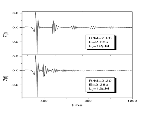
FIG. 1.: The waveforms of the signal emitted by a particle with $(E,L_{z})=(2.38\mu,12\mu M)$ scattered by a star with $R/M=2.26$ (upper panel) and $R/M=2.30$ (lower panel). The excitation of the w-modes is clearly manifested in the signal.

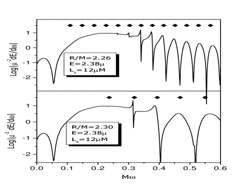
FIG. 2.: The energy spectrum of the signal emitted by a particle with $(E,L_{z})=(2.38\mu,12\mu M)$ scattered by a star with $R/M=2.26$ (upper panel) and $R/M=2.30$ (lower panel). The sharp peaks correspond to the excitation of the w-modes, while the broader peaks at low frequency are mainly contributed by the quadrupole radiation of the particle due to its orbital motion. The diamonds correspond to the real part of the known quasi-normal mode frequencies. It seems that the lowest frequency trapped modes of the first model of star are difficult to be excited.

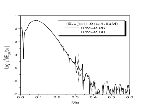
FIG. 3.: The energy spectrum of the signal emitted by a particle with $(E,L_{z})=(1.01\mu,4.5\mu M)$, scattered by a star with $R/M=2.26$ and with $R/M=2.30$. The sharp peaks correspond to the excitation of the various w-modes of the star, whereas the dominant contribution to the emitted energy is that of the quadrupole emission of the scattered particle, which produces the broader peaks at lower frequencies.

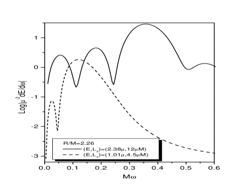
FIG. 4.: The energy spectrum computed by the semirelativistic approximation described in the Appendix, is plotted for two particles with $(E,L_{z})=(2.38\mu,12\mu M)$, and $(E,L_{z})=(1.01\mu,4.5\mu M)$ scattered by a star with $R/M=2.26$. A comparison with the energy spectra given in figures 2 and 3, indicates that the low frequency emission is contributed by the the bremsstrahlung radiation emitted by the accelerated particle.

REFERENCES

- [1] K. Oohara, T.Nakamura, Prog. Theor. Phys. Suppl. 136 , 270, (1999)
- [2] F.A. Rasio, S.L. Shapiro, Class. Quant. Grav. 16, 1, (1999)
- [3] T.W. Baumgarte, S.A. Hughes, S.L. Shapiro, Phys. Rev. D 60, 87501, (1999)
- [4] M. Shibata, K. Uryu, gr-qc/9911058 (1999)
- [5] T.Nakamura, K. Oohara, Y. Kojima, Prog. Theor. Phys. Suppl. 90, 1 (1987)
- [6] R.F.Stark, T.Piran, Phys. Rev. Lett. 55, 891 (1985)
- [7] T.Fond, N.Stergioulas and K.D.Kokkotas MNRAS, 313, 678(2000)
- [8] P.Anninos,D.Hobill, E.Seidel, L.Smarr and W.-M.Suen Phys. Rev. Lett. 71 2851 (1993)
- [9] Y. Kojima, Prog. Theor. Phys. 77, 297 (1987)
- [10] V. Ferrari, L. Gualtieri, and A. Borrelli, Phys. Rev. D 59, 1240 (1999)
- [11] K. Tominaga, M. Saijo, K. Maeda, Phys. Rev. D 60, 24004 (1999)
- [12] Z. Andrade, R. H. Price, Phys. Rev. D 60, 104037 (1999)
- [13] J.Ruoff, P.Laguna and J.Pullin, gr-qc/0005002 (2000)
- [14] S.Chandrasekhar, V.Ferrari, Proc. R. Soc. Lond. A433, 423 (1991)
- [15] Y.Kojima, Phys.Rev. D 46, 4289 (1992)
- [16] N.Andersson and K.D.Kokkotas Phys. Rev. Lett. 77,4134 (1996)
- [17] G.Allen, N.Andersson, K.D.Kokkotas and B.F.Schutz Phys. Rev. D 58, 124012 (1998)
- [18] J.Ruoff Phys. Rev. D in press gr-qc/0003088
- [19] V.Pavlidou, K.Tassis, T.W.Baumgarte, S.L.Shapiro Phys. Rev. D in press gr-qc/0007019
- [20] G.Allen, N.Andersson, K.D.Kokkotas, P.Laguna, J.Pullin and J.Ruoff Phys. Rev. D 60 104021 (1999)
- [21] N.Andersson, K.D.Kokkotas, P.Laguna, Ph.Papadopoulos and M.S.Shipior Phys. Rev. D 60 104021 (1999)
- [22] S.Chandrasekhar, V.Ferrari, Proc. R. Soc. Lond. A432, 247 (1991)
- [23] K.D.Kokkotas, M.N.R.A.S. 268, 1015 (1994); Erratum 277, 1599 (1995)
- [24] R. Ruffini, J. A. Wheeler, Proceedings of the Cortona Symposium on Weak Interaction edited by L. Radicati, Roma, Accademia Nazionale dei Lincei, 169 (1971)