Stochastic backgrounds of gravitational waves

Abstract

We review the motivations for the search of stochastic backgrounds of gravitational waves and we compare the experimental sensitivities that can be reached in the near future with the existing bounds and with the theoretical predictions.

Keywords: Gravitational Waves

PACS numbers: 04.30.-w; 04.30.Db; 04.80.Nn; 98.80.Cq

1 Motivations

A possible target of gravitational wave (GW) experiments is given by stochastic backgrounds of cosmological origin. In a sense, these are the gravitational analog of the 2.7 K microwave photon background and, apart from their obvious intrinsic interest, they would carry extraordinary informations on the state of the very early universe and on physics at correspondingly high energies. To understand this point, one should have in mind the following basic physical principle:

• a background of relic particles gives a snapshot of the state of the universe at the time when these particles decoupled from the primordial plasma.

The smaller is the cross section of a particle, the earlier it decouples. Therefore particles with only gravitational interactions, like gravitons and possibly other fields predicted by string theory, decouple much earlier than particles which have also electroweak or strong interactions. The condition for decoupling is that the interaction rate of the process that mantains equilibrium, $\Gamma$, becomes smaller than the characteristic time scale, which is given by the Hubble parameter $H$,

$$\Gamma\ll H\hskip 28.45274pt\Rightarrow{\rm decoupled}$$ (1)

(we set $\hbar=c=1$). A simple back-of-the-envelope computation shows that, for gravitons,

$$\left(\frac{\Gamma}{H}\right)=\left(\frac{T}{M_{\rm Pl}}\right)^{3}\,,$$ (2)

so that gravitons are decoupled below the Planck scale $M_{\rm Pl}\sim 10^{19}$ GeV, i.e., already $10^{-44}$ sec after the big-bang. This means that a background of GWs produced in the very early universe encodes still today, in its frequency spectrum, all the informations about the conditions in which it was created.

For comparison, the photons that we observe in the CMBR decoupled when the temperature was of order $T\simeq 0.2$ eV, or $3\cdot 10^{5}$ yr after the big bang. This difference in scales simply reflects the difference in the strength of the gravitational and electromagnetic interactions. Therefore, the photons of the CMBR give us a snapshot of the state of the universe at $t\sim 3\cdot 10^{5}$ yr. Of course, from this snapshot we can also understand many things about much earlier epochs. For instance, the density fluctuations present at this epoch have been produced much earlier, and the recent Boomerang data indicate that they are compatible with the prediction from inflation. Therefore, from the photon microwave background we can extract informations on the state of the Universe at much earlier times than the epoch of photon decoupling. In this case, conceptually the situation is similar with trying to understand the aspect that a person had as a child from a picture taken when he was much older. Certainly many features can be inferred from such a picture. Gravitational waves, however, provide directly a picture of the child, and therefore give us really unique informations.

It is clear that the reason why GWs are potentially so interesting is due to their very small cross section, and the very same reason is at the basis of the difficulty of the detection. In the next sections we will review the experimental aspects of the search for stochastic backgrounds and the theoretical expectations. Details and more complete references can be found in ref. [1].

2 Characterization of stochastic backgrounds of GWs

The intensity of a stochastic background of GWs can be characterized by the dimensionless quantity

$$\Omega_{\rm gw}(f)=\frac{1}{\rho_{c}}\,\frac{d\rho_{\rm gw}}{d\log f}\,,$$ (3)

where $\rho_{\rm gw}$ is the energy density of the stochastic background of gravitational waves, $f$ is the frequency ($\omega=2\pi f$) and $\rho_{c}$ is the present value of the critical energy density for closing the universe. In terms of the present value of the Hubble constant $H_{0}$ and Newton’s constant $G_{N}$, the critical density is given by $\rho_{c}=3H_{0}^{2}/(8\pi G_{N})$. The value of $H_{0}$ is usually written as $H_{0}=h_{0}\times 100$ km/(sec–Mpc), where $h_{0}$ parametrizes the existing experimental uncertainty. However, it is not very convenient to normalize $\rho_{\rm gw}$ to a quantity, $\rho_{c}$, which is uncertain: this uncertainty would appear in all the subsequent formulas, although it has nothing to do with the uncertainties on the GW background itself. Therefore, we rather characterize the stochastic GW background with the quantity $h_{0}^{2}\Omega_{\rm gw}(f)$, which is independent of $h_{0}$. All theoretical computations of a relic GW spectrum are actually computations of $d\rho_{\rm gw}/d\log f$ and are independent of the uncertainty on $H_{0}$. Therefore the result of these computations is expressed in terms of $h_{0}^{2}\Omega_{\rm gw}$, rather than of $\Omega_{\rm gw}$.

To understand the effect of the stochastic background on a detector, we need however to think in terms of amplitudes of GWs. A stochastic GW at a given point $\vec{x}=0$ can be expanded, in the transverse traceless gauge, as

$$h_{ab}(t)=\sum_{A=+,\times}\int_{-\infty}^{\infty}df\int d\hat{\Omega}\,\tilde{h}_{A}(f,\hat{\Omega})\,e^{-2\pi ift\,}e_{ab}^{A}(\hat{\Omega})\,,$$ (4)

where $\tilde{h}_{A}(-f,\hat{\Omega})=\tilde{h}_{A}^{*}(f,\hat{\Omega})$. $\hat{\Omega}$ is a unit vector representing the direction of propagation of the wave and $d\hat{\Omega}=d\cos\theta d\phi$. The polarization tensors can be written as $e_{ab}^{+}(\hat{\Omega})=\hat{m}_{a}\hat{m}_{b}-\hat{n}_{a}\hat{n}_{b}\,,e_{ab}^{\times}(\hat{\Omega})=\hat{m}_{a}\hat{n}_{b}+\hat{n}_{a}\hat{m}_{b}\,,$ with $\hat{m},\hat{n}$ unit vectors ortogonal to $\hat{\Omega}$ and to each other. With these definitions, $e^{A}_{ab}(\hat{\Omega})e^{A^{\prime},ab}(\hat{\Omega})=2\delta^{AA^{\prime}}$. For a stochastic background, assumed to be isotropic, unpolarized and stationary, we can define the spectral density $S_{h}(f)$ from the ensemble average of the Fourier amplitudes,

$$\langle\tilde{h}_{A}^{*}(f,\hat{\Omega})\tilde{h}_{A^{\prime}}(f^{\prime},\hat{\Omega}^{\prime})\rangle=\delta(f-f^{\prime})\frac{1}{4\pi}\delta^{2}(\hat{\Omega},\hat{\Omega}^{\prime})\delta_{AA^{\prime}}\frac{1}{2}S_{h}(f)\,,$$ (5)

where $\delta^{2}(\hat{\Omega},\hat{\Omega}^{\prime})=\delta(\phi-\phi^{\prime})\delta(\cos\theta-\cos\theta^{\prime})$. $S_{h}(f)$ has dimensions Hz^-1 and satisfies $S_{h}(f)=S_{h}(-f)$. The choice of normalization is such that

$$\int d\hat{\Omega}d\hat{\Omega}^{\prime}\,\langle\tilde{h}_{A}^{*}(f,\hat{\Omega})\tilde{h}_{A^{\prime}}(f^{\prime},\hat{\Omega}^{\prime})\rangle=\delta(f-f^{\prime})\delta_{AA^{\prime}}\frac{1}{2}S_{h}(f)\,.$$ (6)

$\Omega_{\rm gw}$ and $S_{h}$ are related by

$$\Omega_{\rm gw}(f)=\frac{4\pi^{2}}{3H_{0}^{2}}f^{3}S_{h}(f)\,.$$ (7)

In general, theoretical predictions are expressed more naturally in terms of $h_{0}^{2}\Omega_{\rm gw}(f)$, while the equations involving the signal-to-noise ratio and other issues related to the detection are much more transparent when written in terms of $S_{h}(f)$. Eq. (7) is the basic formula for moving between the two descriptions.

The characteristic amplitude $h_{c}(f)$ is instead defined from

$$\langle h_{ab}(t)h^{ab}(t)\rangle=2\int_{f=0}^{f=\infty}d(\log f)\,\,h_{c}^{2}(f)\,.$$ (8)

$h_{c}(f)$ is dimensionless, and represents a characteristic value of the amplitude, per unit logarithmic interval of frequency. The factor of two on the right-hand side of eq. (8) is part of the definition, and is motivated by the fact that the left-hand side is made up of two contributions, given by $\langle\tilde{h}_{+}^{*}\tilde{h}_{+}\rangle$ and $\langle\tilde{h}_{\times}^{*}\tilde{h}_{\times}\rangle$. In a unpolarized background these contributions are equal, while the mixed term $\langle\tilde{h}_{+}^{*}\tilde{h}_{\times}\rangle$ vanishes, eq. (5). The relation betheen $h_{c}$ and $S_{h}$ is

$$h_{c}^{2}(f)=2fS_{h}(f)\,.$$ (9)

Actually, $h_{c}(f)$ is not yet the most useful dimensionless quantity to use for the comparison with experiments. In fact, any experiment involves some form of binning over the frequency. In a total observation time $T$, the resolution in frequency is $\Delta f=1/T$, so one does not observe $h_{0}^{2}\Omega_{\rm gw}(f)$ but rather

$$\int_{f}^{f+\Delta f}d(\log f)\,\,h_{0}^{2}\Omega_{\rm gw}(f)\simeq\frac{\Delta f}{f}h_{0}^{2}\Omega_{\rm gw}(f)\,,$$ (10)

and, since $h_{0}^{2}\Omega_{\rm gw}(f)\sim f^{3}S_{h}(f)\sim f^{2}h_{c}^{2}(f)$, it is convenient to define

$$h_{c}(f,\Delta f)=h_{c}(f)\left(\frac{\Delta f}{f}\right)^{1/2}\,.$$ (11)

Using $1/(1\,{\rm yr})\simeq 3.17\times 10^{-8}$ Hz as a reference value for $\Delta f$, and $10^{-8}$ as a reference value for $h_{0}^{2}\Omega_{\rm gw}$, one finds

$$h_{c}(f,\Delta f)=7.111\times 10^{-22}\left(\frac{{\rm 1\,mHz}}{f}\right)^{3/2}\left(\frac{h_{0}^{2}\Omega_{\rm gw}(f)}{10^{-8}}\right)^{1/2}\left(\frac{\Delta f}{3.17\times 10^{-8}\,{\rm Hz}}\right)^{1/2}\,.$$ (12)

3 Characterization of the detectors

The response of a detector is characterized by two important quantities: the strain sensitivity $\tilde{h}_{f}$, which gives a measure of the noise in the detector, and the pattern functions $F^{A}(\theta,\phi)$, which reflect the geometry of the detector.

3.1 Strain sensitivity

The total output of the detector $S(t)$ is in general of the form

$$S(t)=s(t)+n(t)$$ (13)

where $n(t)$ is the noise and $s(t)$ is the contribution to the output due to the gravitational waves. Both are taken to be dimensionless quantities. If the noise is gaussian, the ensemble average of the Fourier components of the noise, $\tilde{n}(f)$, satisfies

$$\langle\tilde{n}^{*}(f)\tilde{n}(f^{\prime})\rangle=\delta(f-f^{\prime})\frac{1}{2}S_{n}(f)\,$$ (14)

(actually, non-gaussian noises are potentialy very dangerous in GW experiments, and must be carefully minimized or modelled). The above equation defines the function $S_{n}(f)$, with $S_{n}(-f)=S_{n}(f)$ and dimensions Hz^-1.

The factor $1/2$ is conventionally inserted in the definition so that the total noise power is obtained integrating $S_{n}(f)$ over the physical range $0\leq f<\infty$, rather than from $-\infty$ to $\infty$,

$$\langle n^{2}(t)\rangle=\int_{0}^{\infty}df\,S_{n}(f)\,.$$ (15)

The function $S_{n}$ is known as the spectral noise density. This quantity is quadratic in the noise; it is therefore convenient to take its square root and define the strain sensitivity $\tilde{h}_{f}$

$$\tilde{h}_{f}\equiv\sqrt{S_{n}(f)}\,,$$ (16)

where now $f>0$; $\tilde{h}_{f}$ is linear in the noise and has dimensions Hz^-1/2.

3.2 Pattern functions

GW experiments are designed so that their scalar output $s(t)$ is linear in the GW signal: if $h_{ab}(t)$ is the metric perturbation in the transverse-traceless gauge,

$$s(t)=D^{ab}h_{ab}(t)\,.$$ (17)

$D^{ab}$ is known as the detector tensor. Using eq. (4), we write

$$s(t)=\sum_{A=+,\times}\int_{-\infty}^{\infty}df\int d\hat{\Omega}\,\tilde{h}_{A}(f,\hat{\Omega})\,e^{-2\pi ift}\,D^{ab}e_{ab}^{A}(\hat{\Omega})\,.$$ (18)

It is convenient to define the detector pattern functions $F_{A}(\hat{\Omega})$,

$$F_{A}(\hat{\Omega})=D^{ab}e_{ab}^{A}(\hat{\Omega})\,,$$ (19)

so that

$$s(t)=\sum_{A=+,\times}\int_{-\infty}^{\infty}df\int d\hat{\Omega}\,\tilde{h}_{A}(f,\hat{\Omega})F_{A}(\hat{\Omega})e^{-2\pi ift}\,,$$ (20)

and the Fourier transform of the signal, $\tilde{s}(f)$, is

$$\tilde{s}(f)=\sum_{A=+,\times}\int d\hat{\Omega}\,\tilde{h}_{A}(f,\hat{\Omega})F_{A}(\hat{\Omega})\,.$$ (21)

Explicit expressions for the pattern functions of various detectors can be found in ref. [1].

3.3 Single detectors

For a stochastic background the average of $s(t)$ vanishes and, if we have only one detector, the best we can do is to consider the average of $s^{2}(t)$. Using eqs. (5) and (20),

$$\langle s^{2}(t)\rangle=F\,\int_{0}^{\infty}df\,S_{h}(f)\,,$$ (22)

where

$$F\equiv\int\frac{d\hat{\Omega}}{4\pi}\sum_{A=+,\times}F^{A}(\hat{\Omega})F^{A}(\hat{\Omega})\,$$ (23)

is a factor that gives a measure of the angular efficiency of the detector. For interferometers $F=2/5$, while for cilindrical bars $F=8/15$.

In a single detector a stochastic background will manifest itself as an eccess noise. Comparing eqs. (15) and eq. (22), we see that the signal-to-noise ratio at frequency $f$ is

$${\rm SNR}=\left[\frac{FS_{h}(f)}{S_{n}(f)}\right]^{1/2}\,.$$ (24)

We use the convention that the SNR refers to the GW amplitude, rather than to the GW energy. Since $h_{0}^{2}\Omega_{\rm gw}(f)\sim h_{c}^{2}(f)$ the SNR for the amplitude is the square root of the SNR for the energy, hence the square root in eq. (24).

Using eq. (7) and $S_{n}(f)=\tilde{h}_{f}^{2}$, we can express this result in terms of the minimum detectable value of $h_{0}^{2}\Omega_{\rm gw}$, at a given level of SNR, as

$$h_{0}^{2}\Omega_{\rm gw}^{\rm min}(f)\simeq 10^{-2}\,\frac{({\rm SNR})^{2}}{F}\left(\frac{f}{\rm 100Hz}\right)^{3}\left(\frac{\tilde{h}_{f}}{10^{-22}{\rm Hz}^{-1/2}}\right)^{2}\,.$$ (25)

3.4 Correlated detectors

A much better sensitivity can be obtained correlating two (or more) detectors. In this case we write the output $S_{i}(t)$ of the $i-$th detector as $S_{i}(t)=s_{i}(t)+n_{i}(t)$, where $i=1,2$ labels the detector, and we consider the situation in which the GW signal $s_{i}$ is much smaller than the noise $n_{i}$. We correlate the two outputs defining

$$S_{12}=\int_{-T/2}^{T/2}dt\int_{-T/2}^{T/2}dt^{\prime}\,S_{1}(t)S_{2}(t^{\prime})Q(t-t^{\prime})\,,$$ (26)

where $T$ is the total integration time (e.g. one year) and $Q$ is a real filter function. The simplest choice would be $Q(t-t^{\prime})=\delta(t-t^{\prime})$. However, if one knows the form of the signal that one is looking for, i.e. $S_{h}(f)$, it is possible to optimize the form of the filter function. It turns out that the optimal filter is given by [2, 3, 4, 5, 6]

$$\tilde{Q}(f)=c\frac{\Gamma(f)S_{h}(f)}{S_{n}^{(1)}(f)S_{n}^{(2)}(f)}$$ (27)

with $c$ an arbitrary normalization constant; $S_{h}(f)$ is the spectral density of the signal and $S_{n}^{(i)}(f)$ the noise spectral densities of the two detectors. Since in general $S_{h}(f)$ is not known a priori, one should perform the data analysis considering a set of possible filters. For many cosmological backgrounds, a simple set of power-like filters $S_{h}(f)\sim f^{\alpha}$ should be adequate. Actually, many of the most interesting cosmological backgrounds are expected to be approximately flat within the window of existing or planned experiments.

The function $\Gamma(f)$ in eq. (27) is the (unnormalized) overlap reduction function; it is defined as

$$\Gamma(f)\equiv\int\frac{d\hat{\Omega}}{4\pi}\,\left[\sum_{A}F^{A}_{1}(\hat{\Omega})F^{A}_{2}(\hat{\Omega})\right]\exp\left\{2\pi if\hat{\Omega}\cdot\frac{\Delta\vec{x}}{c}\right\}\,,$$ (28)

where $\Delta\vec{x}$ is the separation between the two detectors. It gives a measure of how well the two detectors are correlated; for instance, if the distance between them is much bigger than the typical wavelength of the stochastic GWs, the two detectors do not really see the same GW backgrounds, and noting is gained correlating them. It also depends on the relative orientation between them.

It is conventional to introduce the (normalized) overlap reduction function $\gamma(f)$ [3, 4]

$$\gamma(f)=\frac{\Gamma(f)}{F_{12}}\,,$$ (29)

where

$$F_{12}\equiv\int\frac{d\hat{\Omega}}{4\pi}\sum_{A}F^{A}_{1}(\hat{\Omega})F^{A}_{2}(\hat{\Omega})|_{\rm aligned}\,.$$ (30)

Here the subscript means that we must compute $F_{12}$ taking the two detectors to be perfectly aligned, rather than with their actual orientation. If the two detectors are of the same type, e.g. two interferometers or two cylindrical bars, $F_{12}$ is the same as the constant $F$ defined in eq. (23). The use of $\Gamma(f)$ is more convenient when we want to write equations that hold independently of what detectors (interferometers, bars, or spheres) are used in the correlation (furthermore, in the case of the correlation between an interferometer and the scalar mode of a sphere $F_{12}=0$, so this normalization is impossible; then, one just uses $\Gamma(f)$, which is the quantity that enters directly in the SNR).

The SNR for two correlated detectors, with optimal filtering, is

$${\rm SNR}=\left[2T\int_{0}^{\infty}df\,\Gamma^{2}(f)\frac{S_{h}^{2}(f)}{S_{n}^{2}(f)}\right]^{1/4}\,.$$ (31)

Comparing with eq. (24) we see that now the SNR is given by an integral over all frequencies, rather then by a comparison of $S_{h}(f)$ with $S_{n}(f)$ at fixed $f$. We denote by $\Delta f$ the frequency range where both detectors are sensitive and at the same time the overlap reduction function $\Gamma(f)$ is not much smaller than one. Then, if the integration time $T$ is such that $T\Delta f\gg 1$, correlating two detectors is much better than working with the single detectors.

Finally, it can be useful to define a dimensionless characteristic noise associated to the correlated detectors. It turns out that the quantity that is meaningful to compare directly to the characteristic dimensionless amplitude $h_{c}(f)$ of the GW (defined in sect. 2) is a characteristic noise $h_{n}(f)$ defined by

$$h_{n}(f)\equiv\frac{1}{(\frac{1}{2}T\Delta f)^{1/4}}\,\left(\frac{fS_{n}(f)}{\Gamma(f)}\right)^{1/2}\,.$$ (32)

The characteristic noise $h_{n}(f)$ is a useful but approximate concept, since the correct expression of the SNR for correlated detectors is obtained integrating over all frequencies, eq. (31), and not comparing $h_{n}(f)$ and $h_{c}(f)$ at fixed $f$.

4 Experiments

4.1 Resonant bars

There are five ultracryogenic resonant bars around the world, in operation since a few years:

detector	location	taking data since
NAUTILUS	Frascati, Rome	1993
EXPLORER	Cern (Rome group)	1990
ALLEGRO	Louisiana, USA	1991
AURIGA	Padua, Italy	1997
NIOBE	Perth, Australia	1993

Table 1: The existing resonant bars.

Compared to interferometers, they are narrow band detectors, since they operate in a frequency band of the order of a few Hz, with resonant frequency of the order of 900 Hz (it should be observed, however, that with recent improvement in the electronics, EXPLORER has now a useful band of the order of a few tens of Hz). Fig. 1 shows the sensitivity curve of NAUTILUS.

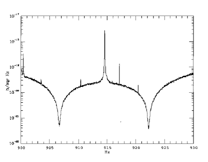
Figure 1: The sensitivity curve of NAUTILUS (courtesy of the NAUTILUS collaboration)

Figure 2: The planned VIRGO sensitivity curve.

4.2 Ground-based interferometers

The first generation of large scale interferometers is presently under construction. LIGO consists of two detectors, in Hanford, Washington, and Livingston, Louisiana, with 4 km arms. VIRGO is under construction near Pisa, and has 3 km arms. Somewhat smaller are GEO600, near Hannover, with 600m arms and TAMA300 in Japan; these smaller interferometers also aim at developing advanced techniques needed for second-generation interferometers. Fig. 2 shows the planned VIRGO sensitivity curve. Interferometers are wide-band detectors, and will cover the region between a few Hertz up to approximately a few kHz. Comparing the data in fig. 2 with eq. (25) we see that used as single detectors, VIRGO and LIGO could measure

$$h_{0}^{2}\Omega_{\rm gw}\raise 1.72218pt\hbox{$>$}\kern-6.99997pt\lower 2.6694pt\hbox{$\sim$}10^{-2}\,.$$ (33)

As discussed in the previous section, much more interesting values can be obtained correlating two interferometers, an interferometer and a bar, or two bars. The values for one year of integration time are given in table 2.

detector 1	detector 2	$h_{0}^{2}\Omega_{\rm gw}$
LIGO-WA	LIGO-LA	$5\times 10^{-6}$
VIRGO	LIGO-LA	$4\times 10^{-6}$
VIRGO	LIGO-WA	$5\times 10^{-6}$
VIRGO	GEO	$5.6\times 10^{-6}$
VIRGO	TAMA	$1\times 10^{-4}$
VIRGO	AURIGA	$4\times 10^{-4}$
VIRGO	NAUTILUS	$7\times 10^{-4}$
AURIGA	NAUTILUS	$5\times 10^{-4}$

Table 2: The sensitivity for various two-detectors correlations.

4.3 Advanced interferometers

The interferometers presently under construction are the first generation of large-scale interferometers, and second generation interferometers, with much better sensitivities, are under study. In particular, the first data from the initial LIGO are expected by 2002, and the improvements leading from the initial LIGO to the advanced detector are expected to take place around 2004-2006.

The overall improvement of LIGOII is expected to be, depending on the frequency, one or two orders of magnitude in $\tilde{h}_{f}$. This is quite impressive, since two order of magnitudes in $\tilde{h}_{f}$ means four order of magnitudes in $h_{0}^{2}\Omega_{\rm gw}(f)$ and therefore interesting sensitivity, $h_{0}^{2}\Omega_{\rm gw}$ of order $10^{-5}$, even for a single detector, without correlations.

Correlating two advanced detectors one could reach extremely interesting values: the sensitivity of the correlation between two advanced LIGO is estimated to be [5]

$$h_{0}^{2}\Omega_{\rm gw}\simeq 5\times 10^{-11}\,.$$ (34)

4.4 The space interferometer LISA

This project, approved by ESA and NASA, is an interferometer which will be sent into space around 2010. Going into space, one is not limited anymore by seismic and gravity-gradient noises; LISA could then explore the very low frequency domain, $10^{-4}$ Hz $<f<1$ Hz. At the same time, there is also the possibility of a very long path length (the mirrors will be freely floating into the spacecrafts at distances of $5\times 10^{6}$ km from each other!), so that the requirements on the position measurement noise can be relaxed. The goal is to reach a strain sensitivity $\tilde{h}_{f}=4\times 10^{-21}\,\,{\rm Hz}^{-1/2}$ at $f=1$ mHz. At this level, one expects first of all signals from galactic binary sources, extra-galactic supermassive black holes binaries and super-massive black hole formation. Concerning the stochastic background, going to low frequencies provides a terrific advantage: eq. (7) tells that

$$\Omega_{\rm gw}(f)\sim f^{3}S_{h}(f)\,.$$ (35)

The ability to perform an interferometric measurement is encoded into the spectral density of the noise, $S_{n}(f)$, and with a single detector we can measure $S_{h}(f)\sim S_{n}(f)$. Then, if we are able to reach a good value of $S_{n}$ at low frequency, eq. (35) shows that we are able to measure a very small value of $\Omega_{\rm gw}$, thanks to the factor $f^{3}$. Going down by a factor $10^{5}$ in frequency, say from 10 Hz to 1 mHz, the factor $f^{3}$ provides an improvement by a factor $10^{15}$! Even used as a single detector, LISA can therefore reach very interesting sensitivities. Indeed, in terms of $h_{0}^{2}\Omega_{\rm gw}$ the sensitivity of LISA corresponds to

$$h_{0}^{2}\Omega_{\rm gw}(f=1\,{\rm mHz})\simeq 1\times 10^{-12}\,.$$ (36)

We can now also understand why it is instead very difficult to build a good detector of stochastic GWs at high frequencies, $f\gg 1$ kHz. One can imagine to build an apparatus that measures extremely small displacements, at high frequencies, so that at some $f\gg 1$ kHz, the spectral density of the noise $S_{n}(f)$ is very small. However, the quantity which is relevant for the comparison with theoretical prediction, and on which strong theoretical bounds exist at all frequencies, is $h_{0}^{2}\Omega_{\rm gw}$, and once one translates the sensitivity in terms of $h_{0}^{2}\Omega_{\rm gw}$, it will be very poor because the factor $f^{3}$ now works in the wrong direction.

5 Bounds on $h_{0}^{2}\Omega_{\rm gw}$

In Fig. 3 we show the most relevant bounds on stochastic GW backgrounds, together with the experimental sensitivities discussed above. On the horizontal axis we cover a huge range of frequencies. The lowest value, $f=10^{-18}$ Hz, corresponds to a wavelength as large as the present Hubble radius of the universe; the highest value shown, $f=10^{12}$ Hz, has instead the following meaning: if we take a graviton produced during the Planck era, with a typical energy of the order of the Planck or string energy scale, and we redshift it to the present time using the standard cosmological model, we find that today it has a frequency of order $10^{11}$ or $10^{12}$ Hz. This value therefore is the maximum possible cutoff of spectra of GWs produced in the very early universe. The maximum cutoff for astrophysical processes is of course much lower, of order 10 kHz [7, 8]. So this huge frequency range encompasses all the GWs that can be considered. Let us now discuss in turn the various bounds.

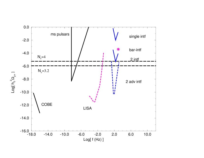
Figure 3: The bounds from nucleosynthesis (horizontal dashed lines, for $N_{\nu}=4$ and for $N_{\nu}=3.2$), from COBE and from ms pulsars, together with the sensitivity of a single ground based detector of the VIRGO or LIGO type (blue solid line), a bar-interferometer correlation (pink star), a 2-interferometer correlation (blue solid line; LIGO-LIGO, LIGO-VIRGO and VIRGO-GEO all give very similar sensitivities), two advanced LIGO correlation (blue dashed line ) and LISA (pink dashed line).

5.1 Nucleosynthesis bound

The outcome of nucleosynthesis depends on a balance between the particle production rates and the expansion rate of the universe, measured by the Hubble parameter $H$. Einstein equation gives $H^{2}\sim G_{N}\rho$, where $\rho$ is the total energy density, including of course $\rho_{\rm gw}$. Nucleosynthesis successfully predicts the primordial abundances of deuterium, ³He, ⁴He and ⁷Li assuming that the only contributions to $\rho$ come from the particles of the Standard Model, and no GW contribution. Therefore, in order not to spoil the agreement, any further contribution to $\rho$ at time of nucleosynthesis, including the contribution of GWs, cannot exceed a maximum value. The bound is usually written in terms of an effective number of neutrino species $N_{\nu}$, and, applied to GWs, reads

$$\int_{f=0}^{f=\infty}d(\log f)\,\,h_{0}^{2}\Omega_{\rm gw}(f)\leq 5.6\times 10^{-6}(N_{\nu}-3)\,.$$ (37)

The limit on $N_{\nu}$ is subject to various systematic errors, which have to do mainly with the issues of how much of the observed ⁴He abundance is of primordial origin, and of the nuclear processing of ³He in stars. Different bounds on $N_{\nu}$ have therefore been proposed. The analysis of ref. [9] gives $N_{\nu}<3.2$ at 95% c.l.; this is shown in fig. 3, together with a more conservative bound $N_{\nu}<4$. Note that the nucleosynthesis bound is really a bound over the total energy density, i.e. over the integral of $h_{0}^{2}\Omega_{\rm gw}(f)$ over $d\log f$. However, if the integral cannot exceed this value, also its positive integrand cannot exceed it over a sizable range of frequencies. The actual bound on $h_{0}^{2}\Omega_{\rm gw}(f)$ depends on its frequency dependence, and if for instance $h_{0}^{2}\Omega_{\rm gw}(f)$ is approximatly constant between two frequencies $f_{\rm min}$ and $f_{\rm max}$, the bound on $h_{0}^{2}\Omega_{\rm gw}$ is stronger by a factor $\sim\log(f_{\rm max}/f_{\rm min})$. Of course, the nucleosynthesis bound applies only to GW produced before nucleosynthesis, and is not relevant for GW of astrophysical origin.

5.2 Bounds from millisecond pulsars

Millisecond pulsar are an extremely impressive source of high precision measurements [10]. For instance, the observations of the first msec pulsar discovered, B1937+21, after 9 yr of data, give a period of $1.557\,806\,468\,819\,794\,5\pm 0.000\,000\,000\,000\,000\,4$ ms. As a consequence, pulsars are also a natural detector of GWs, since a GW passing between us and the pulsar causes a fluctuation in the time of arrival of the pulse, proportional to the GW amplitute $h_{c}(f)$. If the uncertainty in the time of arrival of the pulse is $\epsilon$ and the total observation time is $T$, this ‘detector’ is sensitive to $h_{c}(f)\sim\epsilon/T$, for frequencies $f\sim 1/T$. The highest sensitivities can then be reached for a continuous source, as a stochastic background, after one or more years of integration, and therefore for $f\sim 10^{-9}-10^{-8}$ Hz. Based on the data from PSR B1855+09, ref. [11] gives a limit, at $f\equiv f_{*}=4.4\times 10^{-9}$ Hz (at 90% c.l.),

$$h_{0}^{2}\Omega_{\rm gw}(f_{*})<4.8\times 10^{-9}\,.$$ (38)

Since the resolution on $h_{c}(f)$ is proportional to $1/T$ and $h_{0}^{2}\Omega_{\rm gw}\sim h_{c}^{2}$, the bound for $f>f_{*}$ is

$$h_{0}^{2}\Omega_{\rm gw}(f)<4.8\times 10^{-9}\,\left(\frac{f}{f_{*}}\right)^{2}\,,$$ (39)

and therefore it is quite significant (better than the nucleosynthesis bound) even for $f\sim 10^{2}f_{*}$. For $f<f_{*}$, instead, the pulsar provides no limit at all. With the observation time the bound will improve steadily and will move toward lower and lower frequencies. It is given by the wedge-shaped curve in fig. 3.

5.3 Bound from COBE

Another important constraint comes from the COBE measurement of the fluctuation of the temperature of the cosmic microwave background radiation (CMBR). The basic idea is that a strong background of GWs at very long wavelengths produces a stochastic redshift on the frequencies of the photons of the 2.7K radiation, and therefore a fluctuation in their temperature (Sachs-Wolfe effect). The analysis of refs. [12, 5], where the effect of multipoles with $2\leq l\leq 30$ is included, gives a bound

$$h_{0}^{2}\Omega_{\rm gw}(f)<7\times 10^{-11}\left(\frac{H_{0}}{f}\right)^{2}\,,\hskip 56.9055pt(3\times 10^{-18}\,{\rm Hz}<f<10^{-16}\,{\rm Hz})\,.$$ (40)

This bound is stronger at the upper edge of its range of validity, $f\sim 30H_{0}\sim 10^{-16}$ Hz, where it gives

$$h_{0}^{2}\Omega_{\rm gw}(f)<7\times 10^{-14}\,,\hskip 56.9055pt(f\sim\,10^{-16}\,\rm{Hz})\,.$$ (41)

6 Theoretical predictions

Many cosmological production mechanisms have been proposed in recent years. Four examples are shown in fig. 4:

Inflation. The amplification of vacuum fluctuations at the transition between an inflationary phase and the radiation dominated era produces GWs shown as the curve $(a)$ in fig. 4 and is one of the oldest [13] and most studied examples. The condition that the COBE bound is not exceeded puts a limit on the value of $h_{0}^{2}\Omega_{\rm gw}$ at all frequencies, which is below the experimental sensitivities, even for LISA. So, while it is one of the best studied examples, it appears that it is not very promising from the point of view of detection.

String cosmology. In a cosmological model which follows from the low energy action of string theory [14, 15] the amplification of vacuum fluctuations can give a much stronger signal [16, 17]. The model has two free parameters that reflect our ignorance of the large curvature phase. The curve $(b)$ in fig. 4 shows the very interesting signal that could be obtained for some choice of these parameters, while for other choices the value of $h_{0}^{2}\Omega_{\rm gw}$ at VIRGO/LIGO or at LISA frequencies becomes unobservably small.

Cosmic strings. These are topological defects that can exist in grand unified theories [18], and vibrating, they produce a large amount of GWs, shown in curve $(c)$ of fig. 4. Cosmic strings are characterized by a mass per unit length $\mu$, and the most stringent bound on $G_{N}\mu$ comes from msec pulsars, and it is of order $10^{-6}$.

Phase transitions. Another possible source of GWs is given by phase transitions in the early universe. In particular, a phase transition at the electroweak scale would give a signal just in the LISA frequency window, while the QCD phase transition is expected to give a signal peaked around $f=4\times 10^{-6}$ Hz. However, the signal is sizable only if the phase transition is first order and, unfortunately, in the Standard Model with the existing bounds on the Higgs mass, there is not even a phase transition but rather a smooth crossover, so that basically no GW is produced. However, in supersymmetric extensions of the Standard Model, the transition can be first order, and a stronger signal could be obtained. Depending on the strength of the transition, one could even get a signal such as curve $(d)$ of fig. 4.

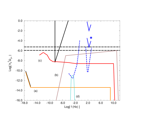
Figure 4: The backgrounds predicted, with optimistic choice of parameters, by (a) inflation, (b) string cosmology, (c) cosmic strings, (d) a first order phase transition at the electroweak scale, together with the bounds and sensitivities of fig. 3.

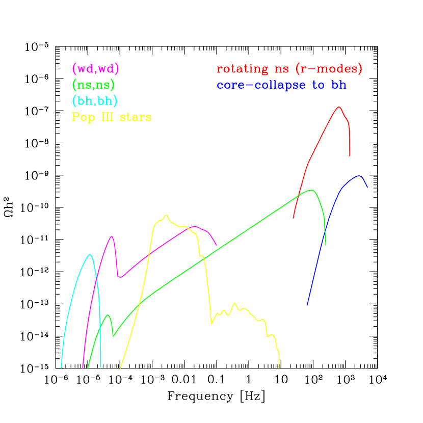
Figure 5: Stochastic backgrounds of astrophysical origin. From left to right, black hole-black hole binaries, white dwarf-white dwarf binaries, neutron star-neeutron star binaries (the curve extending up to $10^{2}$), a pregalactic Population III stars, r-modes of neutron stars and supernova collapse to black holes (figure kindly provided by Raffaella Schneider).

Finally, there are very interesting astrophysical backgrounds, coming from a large number of unresolved sources. These are displayed in fig. 5. For a discussion, see [19] and the contribution of Raffaella Schneider to these proceedings. Another important issue, especially for LISA, is also how to discriminate cosmological from astrophysical backgrounds, see eg. [20].

The conclusion that emerges looking at fig. 3 is that in the next few years, with the first generation of ground based interferometers, we will have the possibility to explore five new order of magnitude in energy densities, probing the content in GWs of the universe down to $h_{0}^{2}\Omega_{\rm gw}\sim 10^{-5}$. At this level, the nucleosynthesis bound suggest that the possibility of detection are quite marginal. It should not be forgotten, however, that nucleosynthesis is a (beautiful) theory, with a lot of theoretical input from nuclear reaction in stars, etc., and its prediction is by no means a substitute for a measurement of GWs. With the second generation of ground based interferometers and with LISA, we will then penetrate quite deeply into a region which experimentally is totally unexplored, and where a number of explicit examples (although subject to large theoretical uncertainties) suggest that a positive result can be found.

References

- [1] M. Maggiore, Phys. Rept. 331 (2000), 283.
- [2] P. Michelson, Mon. Not. Roy. Astron. Soc. 227 (1987) 933.
- [3] N. Christensen, Phys. Rev. D46 (1992) 5250.
- [4] E. Flanagan, Phys. Rev. D48 (1993) 2389.
- [5] B. Allen, The Stochastic Gravity-Wave Background: Sources and Detection, in Les Houches School on Astrophysical Sources of Gravitational Waves, eds. J.A. Marck and J.P. Lasota, (Cambridge University Press, 1996); gr-qc/9604033.
- [6] S. Vitale, M. Cerdonio, E. Coccia and A. Ortolan, Phys. Rev. D55 (1997) 1741.
- [7] K.S. Thorne, in 300 Years of Gravitation, S. Hawking and W. Israel eds., Cambridge University Press, Cambridge, 1987.
- [8] B. F. Schutz, “Low-frequency sources of gravitational waves: A tutorial,” gr-qc/9710079.
- [9] S. Burles, K. M. Nollett, J. N. Truran and M. S. Turner, Phys. Rev. Lett. 82 (1999) 4176.
- [10] D. Lorimer, Binary and Millisecond Pulsars, in Living Reviews in Relativity, available electronically at www.livingreviews.org/Articles/Volume1/1998-10lorimer.
- [11] S. Thorsett and R. Dewey, Phys. Rev. D53 (1996) 3468.
- [12] B. Allen and S. Koranda, Phys. Rev. D50 (1994) 3713.
- [13] L.P. Grishchuk, Sov. Phys. JETP, 40 (1975) 409.
- [14] G. Veneziano, Phys. Lett. B265 (1991) 287.
- [15] M. Gasperini and G. Veneziano, Astropart. Phys. 1 (1993) 317; Mod. Phys. Lett. A8 (1993) 3701. An up-to-date collection of references on string cosmology can be found at http://www.to.infn.it/teorici/ gasperin/
- [16] R. Brustein, M. Gasperini, M. Giovannini and G. Veneziano, Phys. Lett. B361 (1995) 45.
- [17] R. Brustein, M. Gasperini and G. Veneziano, Phys. Rev. D55 (1997) 3882.
- [18] A. Vilenkin and E.P.S. Shellard, Cosmic Strings and other Topological Defects, Cambridge Univ. Press, Cambridge 1994.
- [19] V. Ferrari, S. Matarrese and R. Schneider, Mon. Not. R. Astron. Soc. 303 (1999) 247 and 303 (1999) 258.
- [20] C. Ungarelli and A. Vecchio, High energy physics and the very-early universe with LISA, gr-qc/0003021.