Conversion of conventional gravitational-wave interferometers into QND interferometers by modifying their input and/or output optics

Abstract

The LIGO-II gravitational-wave interferometers ($ca.\ 2006$–2008) are designed to have sensitivities near the standard quantum limit (SQL) in the vicinity of 100 Hz. This paper describes and analyzes possible designs for subsequent, LIGO-III interferometers that can beat the SQL. These designs are identical to a conventional broad-band interferometer (without signal recycling), except for new input and/or output optics. Three designs are analyzed: (i) a squeezed-input interferometer (conceived by Unruh based on earlier work of Caves) in which squeezed vacuum with frequency-dependent (FD) squeeze angle is injected into the interferometer’s dark port; (ii) a variational-output interferometer (conceived in a different form by Vyatchanin, Matsko and Zubova), in which homodyne detection with FD homodyne phase is performed on the output light; and (iii) a squeezed-variational interferometer with squeezed input and FD-homodyne output. It is shown that the FD squeezed-input light can be produced by sending ordinary squeezed light through two successive Fabry-Perot filter cavities before injection into the interferometer, and FD-homodyne detection can be achieved by sending the output light through two filter cavities before ordinary homodyne detection. With anticipated technology (power squeeze factor $e^{-2R}=0.1$ for input squeezed vacuum and net fractional loss of signal power in arm cavities and output optical train $\epsilon_{*}=0.01$) and using an input laser power $I_{o}$ in units of that required to reach the SQL (the planned LIGO-II power, $I_{\rm SQL})$, the three types of interferometer could beat the amplitude SQL at 100 Hz by the following amounts $\mu\equiv\sqrt{S_{h}}/\sqrt{S_{h}^{\rm SQL}}$ and with the following corresponding increase ${\cal V}=1/\mu^{3}$ in the volume of the universe that can be searched for a given non-cosmological source:

Squeezed-Input — $\mu\simeq\sqrt{e^{-2R}}\simeq 0.3$ and ${\cal V}\simeq 1/0.3^{3}\simeq 30$ using $I_{o}/I_{\rm SQL}=1$.

Variational-Output — $\mu\simeq\epsilon_{*}^{1/4}\simeq 0.3$ and ${\cal V}\simeq 30$ but only if the optics can handle a ten times larger power: $I_{o}/I_{\rm SQL}\simeq 1/\sqrt{\epsilon_{*}}=10$.

Squeezed-Varational — $\mu=1.3(e^{-2R}\epsilon_{*})^{1/4}\simeq 0.24$ and ${\cal V}\simeq 80$ using $I_{o}/I_{\rm SQL}=1$; and $\mu\simeq(e^{-2R}\epsilon_{*})^{1/4}\simeq 0.18$ and ${\cal V}\simeq 180$ using $I_{o}/I_{\rm SQL}=\sqrt{e^{-2R}/\epsilon_{*}}\simeq 3.2$.

I Introduction and summary

In an interferometric gravitational-wave detector, laser light is used to monitor the motions of mirror-endowed test masses, which are driven by gravitational waves $h(t)$. The light produces two types of noise: photon shot noise, which it superposes on the interferometer’s output signal, and fluctuating radiation-pressure noise, by which it pushes the test masses in random a manner that can mask their gravity-wave-induced motion. The shot-noise spectral density scales with the light power $I_{o}$ entering the interferometer as $S_{h}^{\rm shot}\propto 1/I_{o}$; the radiation-pressure noise scales as $S_{h}^{\rm rp}\propto I_{o}$.

In the first generation of kilometer-scale interferometers (e.g., LIGO-I, 2002–2003 [1]), the laser power will be low enough that shot-noise dominates and radiation-pressure noise is unimportant. Tentative plans for the next generation interferometers (LIGO-II, ca. 2006–2008) include increasing $I_{o}$ to the point that, $S_{h}^{\rm rp}=S_{h}^{\rm shot}$ at the interferometers’ optimal gravitational-wave frequency, $\Omega/2\pi\sim 100$ Hz. The resulting net noise $S_{h}=S_{h}^{\rm rp}+S_{h}^{\rm shot}=2S_{h}^{\rm shot}$ is the lowest that can be achieved with conventional interferometer designs. Further increases of light power will drive the radiation-pressure on upward, increasing the net noise, while reductions of light power will drive the shot noise upward, also increasing the net noise.

This minimum achievable noise is called the “Standard Quantum Limit” (SQL) [2] and is denoted $S_{h}^{\rm SQL}\equiv h_{\rm SQL}^{2}$. It can be regarded as arising from the effort of the quantum properties of the light to enforce the Heisenberg uncertainty principle on the interferometer test masses, in just the manner of the Heisenberg microscope. Indeed, a common derivation of the SQL is based on the uncertainty principle for the test masses’ position and momentum [3]: The light makes a sequence of measurements of the difference $x$ of test-mass positions. If a measurement is too accurate, then by state reduction it will narrow the test-mass wave function so tightly ($\Delta x$ very small) that the momentum becomes highly uncertain (large $\Delta p$), producing a wave-function spreading that is so rapid as to create great position uncertainty at the time of the next measurement. There is an optimal accuracy for the first measurement—an accuracy that produces only a factor $\sqrt{2}$ spreading and results in optimal predictability for the next measurement. This optimal accuracy corresponds to $h_{\rm SQL}$.

Despite this apparent intimate connection of the SQL to test-mass quantization, it turns out that the test-mass quantization has no influence whatsoever on the output noise in gravitational-wave interferometers [4]. The sole forms of quantum noise in the output are photon shot noise and photon radiation-pressure noise.

Vladimir Braginsky (the person who first recognized the existence of the SQL for gravitational-wave detectors and other high-precision measuring devices [5]) realized, in the mid 1970s, that the SQL can be overcome, but to do so would require significant modifications of the experimental design. Braginsky gave the name Quantum Nondemolition (QND) to devices that can beat the SQL; this name indicates the ability of QND devices to prevent their own quantum properties from demolishing the information one is trying to extract [6].

The LIGO-I interferometers are now being assembled at the LIGO sites, in preparation for the first LIGO gravitational-wave searches. In parallel, the LIGO Scientific Community (LSC) is deeply immersed in R&D for the LIGO-II interferometers [7], and a small portion of the LSC is attempting to invent practical designs for the third generation of interferometers, LIGO-III. This paper is a contribution to the LIGO-III design effort.

In going from LIGO-II to LIGO-III, a large number of noise sources must be reduced. Perhaps the most serious are the photon shot noise and radiation pressure noise (“optical noise”), and thermal noise in the test masses and their suspensions [7, 8]. In this paper we shall deal solely with the shot noise and radiation pressure noise (and the associated SQL); we shall tacitly assume that all other noise sources, including thermal noise, can be reduced sufficiently to take full advantage of the optical techniques that we propose and analyze.

Because LIGO-II is designed to operate at the SQL, in moving to LIGO-III there are just two ways to reduce the optical noise: increase the masses $m$ of the mirrored test masses (it turns out that $h_{\rm SQL}^{2}\propto 1/m$), or redesign the interferometers so they can perform QND. The transition from LIGO-I to LIGO-II will already (probably) entail a mass increase, from $m=11$ kg to $m=30$ kg, in large measure because the SQL at 11 kg was unhappily constraining [7]. Any large further mass increase would entail great danger of unacceptably large noise due to energy coupling through the test-mass suspensions and into or from the overhead supports (the seismic isolation system); a larger mass would also entail practical problems due to the increased test-mass dimensions. Accordingly, there is strong motivation for trying to pursue the QND route.

Our Caltech and Moscow-University research groups are jointly exploring three approaches to QND interferometer design:

• The conversion of conventional interferometers into QND interferometers by modifying their input and/or output optics [this paper]. This approach achieves QND by creating and manipulating correlations between photon shot noise and radiation pressure noise; see below. It is the simplest of our three approaches, but has one serious drawback: an uncomfortably high light power, $W_{\rm circ}\gtrsim 1$ MW, that must circulate inside the interferometers’ arm cavities [9]. It is not clear whether the test-mass mirrors can be improved sufficiently to handle this high a power in a sufficiently noise-free way.

• A modification of the interferometer design (including using two optical cavities in each arm) so as to make its output signal be proportional to the relative speeds of the test masses rather than their relative positions [10, 11]. Since the test-mass speed is proportional to momentum, and momentum (unlike position) is very nearly conserved under free test-mass evolution on gravity-wave timescales ($\sim 0.01$ sec), the relative speed is very nearly a “QND observable” [12] and thus is beautifully suited to QND measurements. Unfortunately, the resulting speed-meter interferometer, like our input-output-modified interferometers, suffers from a high circulating light power [9], $W_{\rm circ}\gtrsim 1$ MW.

• Radical redesigns of the interferometer aimed at achieving QND performance with $W_{\rm circ}$ well below 1 MW [13]. These, as currently conceived by Braginsky, Gorodetsky and Khalili, entail transfering the gravitational-wave signal to a single, small test mass via light pressure, and using a local QND sensor to read out the test mass’s motions relative to a local inertial frame.

In this paper we explore the first approach. The foundation for this approach is the realization that: (i) photon shot noise and radiation-pressure noise together enforce the SQL only if they are uncorrelated; see, e.g., Ref. [4]; (ii) whenever carrier light with side bands reflects off a mirror (in our case, the mirrors of an interferometer’s arm cavities), the reflection ponderomotively squeezes the light’s side bands, thereby creating correlations between their radiation-pressure noise in one quadrature and shot noise in the other; (iii) these correlations are not accessed by a conventional interferometer because of the particular quadrature that its photodiode measures; (iv) however, these correlations can be accessed by (conceptually) simple modifications of the interferometer’s input and/or output optics, and by doing so one can beat the SQL. These correlations were first noticed explicitly by Unruh [14], but were present implicitly in Braginsky’s earlier identification of the phenomenon of ponderomotive squeezing [15, 16].

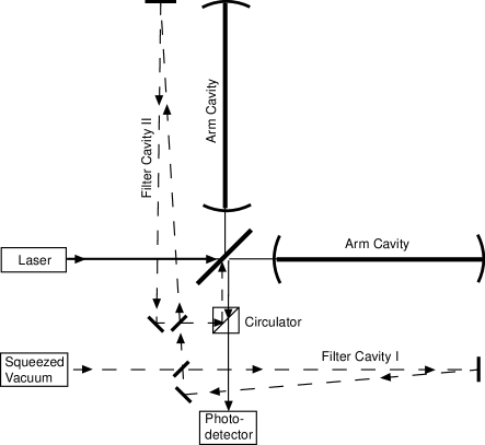
FIG. 1.: Schematic diagram of a squeezed-input interferometer.

In this paper we study three variants of QND interferometers that rely on ponderomotive-squeeze correlations:

(i) Squeezed-Input Interferometer: Unruh [14] (building on earlier work of Caves [17]) invented this design nearly 20 years ago, and since then it has been reanalyzed by several other researchers [18, 19]. In this design, squeezed vacuum is sent into the dark port of the interferometer (“modified input”) and the output light is monitored with a photodetector as in conventional interferometers.

For a broad-band squeezed-input interferometer, the squeeze angle must be a specified function of frequency that changes significantly across the interferometer’s operating gravity-wave band. (This contrasts with past experiments employing squeezed light to enhance interferometry [20, 21], where the squeeze angle was constant across the operating band.) Previous papers on squeezed-input interferometers have ignored the issue of how, in practice, one might achieve the required frequency-dependent (FD) squeeze angle. In Sec. V C, we show that it can be produced via ordinary, frequency-independent squeezing (e.g., by nonlinear optics [22]), followed by filtration through two Fabry-Perot cavities with suitably adjusted bandwidths and resonant-frequency offsets from the light’s carrier frequency. A schematic diagram of the resulting squeezed-input interferometer is shown in Fig. 1 and is discussed in detail below. Our predicted performance for such an interferometer agrees with that of previous research.

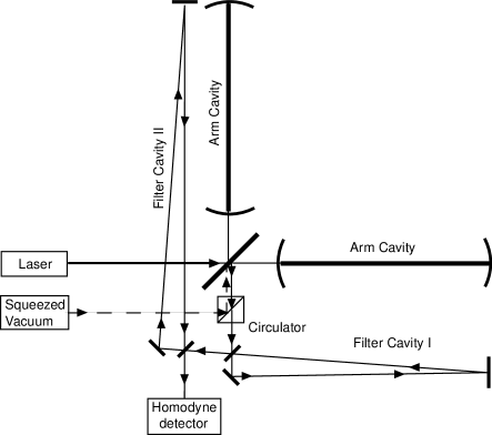
FIG. 2.: Schematic diagram of a squeezed-variational interferometer. A variational-output interferometer differs from this solely by replacing the input squeezed vacuum by ordinary vacuum.

(ii) Variational-Output Interferometer: Vyatchanin, Matsko and Zubova invented this design conceptually in the early 1990’s [23, 24, 25]. It entails a conventional interferometer input (ordinary vacuum into the dark port), but a modified output: instead of photodetection, one performs homodyne detection with a homodyne phase that depends on frequency in essentially the same way as the squeeze angle of a squeezed-input interferometer. Vyatchanin, Matsko and Zubova did not know how to achieve FD homodyne detection in practice, so they proposed approximating it by homodyne detection with a time-dependent (TD) homodyne phase. Such TD homodyne detection can beat the SQL, but (by contrast with FD homodyne) it is not well-suited to gravitational-wave searches, where little is known in advance about the gravitational waveforms or their arrival times. In this paper (Sec. V and Appendix C), we show that the desired FD homodyne detection can be achieved by sending the interferometer’s output light through two successive Fabry-Perot cavities that are essentially identical to those needed in our variant of a squeezed-input interferometer, and by then performing conventional homodyne detection with fixed homodyne angle. A schematic diagram of the resulting variational-output interferometer is shown in Fig. 2.

(iii) Squeezed-Variational Interferometer: This design (not considered in the previous literature) is the obvious combination of the first two; one puts squeezed vacuum into the dark port and performs FD homodyne detection on the output light. The optimal performance is achieved by squeezing the input at a fixed (frequency-independent) angle; filtration cavities are needed only at the output (for the FD homodyne detection) and not at the input; cf. Fig. 2.

In Sec. IV we compute the spectral density of the noise for all three designs, ignoring the effects of optical losses. We find (in agreement with previous analyses [18, 19]) that, when the FD squeeze angle is optimized, the squeezed-input interferometer has its shot noise and radiation-pressure noise both reduced in amplitude (at fixed light power) by $e^{-R}$, where $R$ is the (frequency-independent) squeeze factor; see Fig. 2 below. This enables a lossless squeezed-input interferometer to beat the SQL by a factor $e^{-R}$ (when the power is optimized) but no more. By contrast, the lossless, variational-output interferometer, with optimized FD homodyne phase, can have its radiation-pressure noise completely removed from the output signal, and its shot noise will scale with light power as $1/\sqrt{I_{o}}$ as for a conventional interferometer. As a result, the lossless variational-output interferometer can beat the SQL in amplitude by $\sqrt{I_{\rm SQL}/2I_{o}}$, where $I_{\rm SQL}$ is the light power required by a conventional interferometer to reach the SQL. The optimized, lossless, squeezed-variational interferometer has its radiation-pressure noise completely removed, and its shot noise reduced by $e^{-R}$, so it can beat the SQL in amplitude by $e^{-R}\sqrt{I_{\rm SQL}/2I_{o}}$.

Imperfections in squeezing, in the filter cavities, and in the homodyne local-oscillator phase will produce errors $\Delta\lambda$ in the FD squeeze angle $\lambda(\Omega)$ of a squeezed-input or squeezed-variational interferometer, and $\Delta\zeta$ in the FD homodyne phase $\zeta(\Omega)$ of a variational-output or squeezed-variational interferometer. At the end of Sec. VI E, we shall show that, to keep these errors from seriously compromising the most promising interferometer’s performance, $|\Delta\lambda|$ must be no larger than $\sim 0.05$ radian, and $|\Delta\zeta|$ must be no larger than $\sim 0.01$ radian. This translates into constraints of order five percent on the accuracies of the filter cavity finesses and about 0.01 on their fractional frequency offsets and on the homodyne detector’s local-oscillator phase.

The performance will be seriously constrained by unsqueezed vacuum that leaks into the interferometer’s optical train at all locations where there are optical losses, whether those losses are fundamentally irreversible (e.g. absorption) or reversible (e.g. finite transmissivity of an arm cavity’s end mirror). We explore the effects of such optical losses in Sec. VI. The dominant losses and associated noise production occur in the interferometer’s arm cavities and FD filter cavities. The filter cavities’ net losses and noise will dominate unless the number of bounces the light makes in them is minimized by making them roughly as long as the arm cavities. This suggests that they be 4km long and reside in the beam tubes alongside the interferometer’s arm cavities. To separate the filters’ inputs and outputs, they might best be triangular cavities with two mirrors at the corner station and one in the end station.

Our loss calculations reveal the following:

The squeezed-input interferometer is little affected by losses in the interferometer’s arm cavities or in the output optical train. However, losses in the input optical train (most seriously the filter cavities and a circulator) influence the noise by constraining the net squeeze factor $e^{-2R}$ of the light entering the arm cavities. The resulting noise, expressed in terms of $e^{-2R}$, is the same as in a lossless squeezed-input interferometer (discussed above): With the light power optimized so $I_{o}=I_{\rm SQL}$, the squeezed-input interferometer can beat the amplitude SQL by a factor $\mu\equiv\sqrt{S_{h}}/\sqrt{S_{h}^{\rm SQL}}\simeq\sqrt{e^{-2R}}\simeq 0.3$ (where $e^{-2R}\simeq 0.1$ is a likely achievable value of the power squeeze factor).

The variational-output and squeezed-variational interferometers are strongly affected by losses in the interferometer’s arm cavities and in the output optical train (most seriously: a circulator, the two filter cavities, the mixing with the homodyne detector’s local-oscillator field, and the photodiode inefficiency). The net fractional loss $\epsilon_{*}$ of signal power and (for squeezed-variational) the squeeze factor $e^{-2R}$ for input power together determine the interferometer’s optimized performance: The amplitude SQL can be beat by an amount $\mu=(e^{-2R}\epsilon_{*})^{1/4}$, and the input laser power required to achieve this optimal performance is $I_{o}/I_{\rm SQL}\simeq\sqrt{e^{-2R}/\epsilon_{*}}$. In particular, the variational-output interferometer (no input squeezing; $e^{-2R}=1$), with the likely achievable loss level $\epsilon_{*}=0.01$, can beat the SQL by the same amount as our estimate for the squeezed-input interferometer, $\mu\simeq\epsilon_{*}^{1/4}\simeq 0.3$, but requires ten times higher input optical power, $I_{o}/I_{\rm SQL}\simeq 1/\sqrt{\epsilon_{*}}\simeq 10$ — which could be a very serious problem. By contrast, the squeezed-variational interferometer with the above parameters has an optimized performance $\mu\simeq(0.1\times 0.01)^{1/4}\simeq 0.18$ (substantially better than squeezed-input or variational-output), and achieves this with an optimizing input power $I_{o}/I_{\rm SQL}=\sqrt{0.1/0.01}\simeq 3.2$. If the input power is pulled down from this optimizing value to $I_{o}/I_{\rm SQL}=1$ so it is the same as for the squeezed-input interferometer, then the squeezed-variational performance is debilitated by a factor 1.3, to $\mu\simeq 0.24$, which is still somewhat better than for squeezed-input.

It will require considerable R&D to actually achieve performances at the above levels, and there could be a number of unknown pitfalls along the way. For example, ponderomotive squeezing, which underlies all three of our QND configurations, has never yet been seen in the laboratory and may entail unknown technical difficulties.

Fortunately, the technology for producing squeezed vacuum via nonlinear optics is rather well developed [22] and has even been used to enhance the performance of interferometers [20, 21]. Moreover, much effort is being invested in the development of low-loss test-mass suspensions, and this gives the prospect for new (ponderomotive) methods of generating squeezed light that may perform better than traditional nonlinear optics. These facts, plus the fact that, in a squeezed-input configuration, the output signal is only modestly squeezed and thus is not nearly so delicate as the highly-squeezed output of an optimally performing squeezed-variational configuration, make us feel more confident of success with squeezed-input interferometers than with squeezed-variational ones.

On the other hand, the technology for a squeezed-variational interferometer is not much different from that for a squeezed-input one: Both require input squeezing and both require filter cavities with roughly the same specifications; the only significant differences are the need for conventional, frequency-independent homodyne detection in the squeezed-variational interferometer, and its higher-degree of output squeezing corresponding to higher sensitivity. Therefore, the squeezed-variational interferometer may turn out to be just as practical as the squeezed-input, and may achieve significantly better overall performance at the same laser power.

This paper is organized as follows: In Sec. II we sketch our mathematical description of the interferometer, including our use of the Caves-Schumaker [26, 27] formalism for two-photon quantum optics, including light squeezing (cf. Appendix A); and we write down the interferometer’s input-output relation in the absence of losses [Eq. (23); cf. Appendix B for derivation]. In Sec. III, relying on our general lossless input-output relation (23), we derive the noise spectral density $S_{h}(f)$ for a conventional interferometer and elucidate thereby the SQL. In Sec. IV, we describe mathematically our three QND interferometer designs and, using our lossless input-output relation (23), derive their lossless noise spectral densities. In Sec. V, we show that FD homodyne detection can be achieved by filtration followed by conventional homodyne detection, and in Appendix C we show that the required filtration can be achieved by sending the light through two successive Fabry-Perot cavities with suitably chosen cavity parameters. We list and discuss the required cavity parameters in Sec. V. In Sec. VI, we compute the effects of optical losses on the interferometers’ noise spectral density; our computation relies on an input-output relation (131) and (137) derived in Appendix B. In Sec. VII we discuss and compare the noise performances of our three types of inteferometers. Finally, in Sec. VIII we briefly recapitulate and then list and briefly discuss a number of issues that need study, as foundations for possibly implementing these QND interferometers in LIGO-III.

This paper assumes that the reader is familiar with modern quantum optics and its theoretical tools as presented, for example, in Refs. [28].

II Mathematical Description of the Interferometer

A Input and Output fields

Figure 3 shows the standard configuration for a gravitational-wave interferometer. In this subsection we focus on the beam splitter’s input and output. In our equations we idealize the beam splitter as infinitesimally thin and write the input and output fields as functions of time (not time and position) at the common centers of the beams as they strike the splitter.

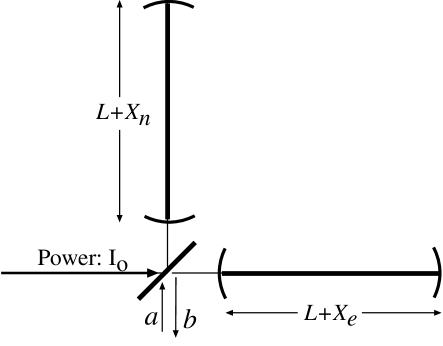
FIG. 3.: Gravitational-wave interferometer with two inputs (the carrier which has power $I_{o}$ entering the bright port, and quantum field $a$ entering the dark port) and one relevant output (the quantum field $b$ leaving the dark port).

At the beam splitter’s bright port the input is a carrier field, presumed to be in a perfectly coherent state with power $I_{o}\sim 10$ kW (achieved via power recycling[29]), angular frequency $\omega_{o}\simeq 1.78\times 10^{15}{\rm sec}^{-1}$ (1.06 micron light), and excitation confined to the $\cos(\omega_{o}t)$ quadrature (i.e., the mean field arriving at the beam splitter is proportional to $\cos(\omega_{o}t)$).

At the dark port the input is a (quantized) electromagnetic field with the positive-frequency part of the electric field given by the standard expression

$$E^{(+)}_{\rm in}=\int_{0}^{\infty}\sqrt{{2\pi\hbar\omega\over{\cal A}c}}\;a_{\omega}e^{-i\omega t}{d\omega\over 2\pi}\;.$$ (1)

Here $\cal A$ is the effective cross sectional area of the beam and $a_{\omega}$ is the annihilation operator, whose commutation relations are

$$[a_{\omega},a_{\omega^{\prime}}]=0\;,\quad[a_{\omega},a_{\omega^{\prime}}^{{\dagger}}]=2\pi\delta(\omega-\omega^{\prime})\;.$$ (2)

Throughout this paper we use the Heisenberg Picture, so $E^{(+)}$ evolves with time as indicated. However, our creation and annihilation operators $a_{\omega}$ and $a_{\omega}^{{\dagger}}$ are fixed in time, with their usual Heisenberg-Picture time evolutions always factored out explicitly as in Eq. (1).

We split the field (1) into side bands about the carrier frequency $\omega_{o}$, $\omega=\omega_{o}\pm\Omega$, with side-band frequencies $\Omega$ in the gravitational-wave range $\sim 60$ to $\sim 6000{\rm sec}^{-1}$ (10 to 1000 Hz), and we define

$$a_{+}\equiv a_{\omega_{o}+\Omega}\;,\quad a_{-}\equiv a_{\omega_{o}-\Omega}\;.$$ (3)

As in Eq. (2), we continue to use a prime on the subscript to denote frequency $\Omega^{\prime}$: $a_{+^{\prime}}\equiv a_{\omega_{o}+\Omega^{\prime}}$. Correspondingly, the commutation relations (2) imply for the only nonzero commutators

$$[a_{+},a_{+^{\prime}}^{{\dagger}}]=2\pi\delta(\Omega-\Omega^{\prime})\;,\;\;[a_{-},a_{-^{\prime}}^{{\dagger}}]=2\pi\delta(\Omega-\Omega^{\prime})\;;$$ (4)

and expression (1) for the dark-port input field becomes

$$E^{(+)}_{\rm in}=\sqrt{2\pi\hbar\omega_{o}\over{\cal A}c}e^{-i\omega_{o}t}\int_{0}^{\infty}\left(a_{+}e^{-i\Omega t}+a_{-}e^{+i\Omega t}\right){d\Omega\over 2\pi}\;.$$ (5)

Here (and throughout this paper) we approximate $\omega_{0}\pm\Omega\simeq\omega_{o}$ inside the square root, since $\Omega/\omega_{o}\sim 3\ 10^{-13}$ is so small; and we formally extend the integrals over $\Omega$ to infinity, for ease of notation.

Because the radiation pressure in the optical cavities produces squeezing, and because this ponderomotive squeezing is central to the operation of our interferometers, we shall find it convenient to think about the interferometer not in terms of the single-photon modes, whose annihilation operators are $a_{+}$ and $a_{-}$, but rather in terms of the correlated two-photon modes (Appendix A and Refs. [26, 27]) whose field amplitudes are

$$a_{1}={a_{+}+a_{-}^{{\dagger}}\over\sqrt{2}}\;,\quad a_{2}={a_{+}-a_{-}^{{\dagger}}\over\sqrt{2}i}\;.$$ (6)

The commutation relations (4) imply the following values for the commutators of these field amplitudes and their adjoints:

$$[a_{1},a_{2^{\prime}}^{{\dagger}}]=-[a_{2},a_{1^{\prime}}^{{\dagger}}]\;=i2\pi\delta(\Omega-\Omega^{\prime})$$ (8)

and all others vanish (though some would be of order $(\Omega/\omega_{o})$ if we had not approximated $\omega_{o}\pm\Omega\simeq\omega_{o}$ inside the square root in Eq. (5); cf. [26, 27]):

$$\;[a_{1},a_{1^{\prime}}]=[a_{1},a_{1^{\prime}}^{{\dagger}}]=[a_{1}^{{\dagger}},a_{1^{\prime}}^{{\dagger}}]=[a_{1},a_{2^{\prime}}]=[a_{1}^{{\dagger}},a_{2^{\prime}}^{{\dagger}}]=0\;,$$ (9)

and similarly with $1\leftrightarrow 2$. In terms of these two-photon amplitudes, Eq. (5) and $E^{(-)}=E^{(+){\dagger}}$ imply that the full electric field operator for the dark-port input is

$$E_{\rm in} = E^{(+)}_{\rm in}+E^{(-)}_{\rm in}$$ (10)

$$= \sqrt{4\pi\hbar\omega_{o}\over{\cal A}c}\left[\cos(\omega_{o}t)\int_{0}^{\infty}\left(a_{1}e^{-\i\Omega t}+a_{1}^{{\dagger}}e^{+i\Omega t}\right){d\Omega\over 2\pi}\right.$$ (12)

$$\quad\quad+\left.\sin(\omega_{o}t)\int_{0}^{\infty}\left(a_{2}e^{-\i\Omega t}+a_{2}^{{\dagger}}e^{+i\Omega t}\right){d\Omega\over 2\pi}\right]\;.$$

Thus, we see that $a_{1}$ is the field amplitude for photons in the $\cos\omega_{o}t$ quadrature and $a_{2}$ is that for photons in the $\sin\omega_{o}t$ quadrature [26, 27]. These and other quadratures will be central to our analysis.

The output field at the beam splitter’s dark port is described by the same equations as the input field, but with the annihilation operators $a$ replaced by $b$; for example,

$$E_{\rm out} = \sqrt{4\pi\hbar\omega_{o}\over{\cal A}c}\left[\cos(\omega_{o}t)\int_{0}^{\infty}\left(b_{1}e^{-\i\Omega t}+b_{1}^{{\dagger}}e^{+i\Omega t}\right){d\Omega\over 2\pi}\right.$$ (14)

$$\quad\quad+\left.\sin(\omega_{o}t)\int_{0}^{\infty}\left(b_{2}e^{-\i\Omega t}+b_{2}^{{\dagger}}e^{+i\Omega t}\right){d\Omega\over 2\pi}\right]\;.$$

We shall find it convenient to introduce explicitly the cosine and sine quadratures of the output field, $E_{1}(t)$ and $E_{2}(t)$, defined by

$$E_{\rm out} = E_{1}(t)\cos(\omega_{o}t)+E_{2}(t)\sin(\omega_{o}t)\;;$$ (15)

$$E_{j}(t) = \sqrt{4\pi\hbar\omega_{o}\over{\cal A}c}\int_{0}^{\infty}\left(b_{j}e^{-\i\Omega t}+b_{j}^{{\dagger}}e^{+i\Omega t}\right){d\Omega\over 2\pi}\;.$$ (16)

TABLE I.: Interferometer parameters and their fiducial values.

Parameter	Symbol	Fiducial Value
light frequency	$\omega_{o}$	$1.8\times 10^{15}{\rm s}^{-1}$
arm cavity ${1\over 2}$-bandwidth	$\gamma$	$2\pi\times 100{\rm s}^{-1}$
grav’l wave frequency	$\Omega$	—
mirror mass	$m$	30 kg
arm length	$L$	4 km
light power to beam splitter	$I_{o}$	—
light power to reach SQL	$I_{\rm SQL}$	$1.0\times 10^{4}$ W
grav’l wave SQL	$h_{\rm SQL}$	$2\times 10^{-24}(\gamma/\Omega){\rm Hz}^{-{1/2}}$
opto-mech’l coupling const	${\cal K}$	${(I_{o}/I_{\rm SQL})2\gamma^{4}\over\Omega^{2}(\gamma^{2}+\Omega^{2})}$
fractional signal-power loss	$\epsilon_{*}$	0.01
max power squeeze factor	$e^{-2R}$	$0.1$

B Interferometer arms and gravitational waves

LIGO’s interferometers are generally optimized for the waves from inspiraling neutron-star and black-hole binaries—sources that emit roughly equal power into all logarthmic frequency intervals $\Delta\Omega/\Omega\sim 1$ in the LIGO band $\sim 10\hbox{Hz}\lesssim f\equiv\Omega/2\pi\lesssim 1000\hbox{Hz}$. Optimization turns out to entail making the lowest point in the interferometer’s dimensionless noise spectrum $f\times S_{h}(f)$ as low as possible. Because of the relative contributions of shot noise, radiation pressure noise, and thermal noise, this lowest point turns out to be at $f\equiv\Omega/2\pi\simeq 100$ Hz. To minimize the noise at this frequency, one makes the end mirrors of the interferometer’s arm cavities (Fig. 3) as highly reflecting as possible (we shall idealize them as perfectly reflecting until Sec. VI), and one gives their corner mirrors transmisivities $T\simeq 0.033$, so the cavities’ half bandwidths are

$$\gamma\equiv{Tc\over 4L}\simeq 2\pi\times 100{\rm Hz}\;.$$ (17)

Here $L=4$ km is the cavities’ length (the interferometer “arm length”). We shall refer to $\gamma$ as the interferometer’s optimal frequency, and when analyzing QND interferometers, we shall adjust their parameters so as to beat the SQL by the maximum possible amount at $\Omega=\gamma$. In Table I we list $\gamma$, $L$ and other parameters that appear extensively in this paper, along with their fiducial numerical values.

In this and the next few sections we assume, for simplicity, that the mirrors and beam splitter are lossless; we shall study the effects of losses in Sec. VI below. We assume that the carrier light (frequency $\omega_{o}$) exites the arm cavities precisely on resonance.

We presume that all four mirrors (“test masses”) have masses $m\simeq 30$ kg, as is planned for LIGO-II.

We label the two arms $n$ for north and $e$ for east, and denote by $X_{n}$ and $X_{e}$ the changes in the lengths of the cavities induced by the test-mass motions. We denote by

$$x\equiv X_{n}-X_{e}$$ (18)

the changes in the arm-length difference, and we regard $x$ as a quantum mechanical observable (though it could equally well be treated as classical [4]). In the absence of external forces, we idealize $x$ as behaving like a free mass (no pendular restoring forces). This idealization could easily be relaxed, but because all signals below $\sim 10$ Hz are removed in the data analysis, the pendular forces have no influence on the interferometer’s ultimate performance.

The arm-length difference evolves in response to the gravitational wave and to the back-action influence of the light’s fluctuating radiation pressure. Accordingly, we can write it as

$$x(t)=x_{o}+{p_{o}\over m/4}t+\int_{-\infty}^{+\infty}(Lh+x_{\rm BA})e^{-i\Omega t}{d\Omega\over 2\pi}\;.$$ (19)

Here $x_{o}$ is the initial value of $x$ when a particular segment of data begins to be collected, $p_{o}$ is the corresponding initial generalized momentum, $m/4$ is the reduced mass associated with the test-mass degree of freedom $x$, $h$ is the Fourier transform of the gravitational-wave field

$$h(t)=\int_{-\infty}^{+\infty}he^{-i\Omega t}{d\Omega\over 2\pi}\;,$$ (20)

and $x_{\rm BA}$ is the influence of the radiation-pressure back action. Notice our notation: $x$, $x_{\rm BA}$ and $h$ are the $\Omega$-dependent Fourier transforms of $x(t)$, $x_{\rm BA}(t)$ and $h(t)$.

Elsewhere [4] we discuss the fact that $x_{o}$ and $p_{o}$ influence the interferometer output only near zero frequency $\Omega\sim 0$, and their influence is thus removed when the output data are filtered. For this reason, we ignore them and rewrite $x(t)$ as

$$x(t)=\int_{-\infty}^{+\infty}(Lh+x_{\rm BA})e^{-i\Omega t}{d\Omega\over 2\pi}\;.$$ (21)

C Output field expressed in terms of input

Because we have idealized the beam splitter as infinitesimally thin, the input field emerging from it and traveling toward the arm cavities has the coherent laser light in the same $\cos\omega_{o}t$ quadrature as the dark-port field amplitude $a_{1}$. We further idealize the distances between the beam splitter and the arm-cavity input mirrors as integral multiples of the carrier wavelength $\lambda_{o}=2\pi c/\omega_{o}$ and as small compared to $2\pi c/\gamma\sim 300{\rm m}$. (These idealizations could easily be relaxed without change in the ultimate results.)

Relying on these idealizations, we show in Appendix B that the annihilation operators $b_{j}$ for the beam splitter’s output quadrature fields $E_{j}(t)$ are related to the input annihilation operators $a_{j}$ and the gravitational-wave signal $h$ by the linear relations

$$b_{1} = \Delta b_{1}=a_{1}e^{2i\beta}\;,$$ (22)

$$b_{2} = \Delta b_{2}+\sqrt{2{\cal K}}{h\over h_{\rm SQL}}e^{i\beta}\;,\quad\Delta b_{2}=(a_{2}-{\cal K}a_{1})e^{2i\beta}\;.$$ (23)

Here and below, for any operator $A$, $\Delta A\equiv A-\langle A\rangle$. This input-output equation and the quantities appearing in it require explanation.

The quantities $\Delta b_{j}$ are the noise-producing parts of $b_{j}$, which remain when the gravitational-wave signal is turned off. The $a_{j}$ impinge on the arm cavities at a frequency $\omega_{o}+\Omega$ that is off resonance, so they acquire the phase shift $2\beta$ upon emerging, where

$$\beta\equiv\arctan(\Omega/\gamma)\;.$$ (24)

If the test masses were unable to move, then $\Delta b_{j}$ would just be $a_{j}e^{2i\beta}$; however, the fluctuating light pressure produces the test-mass motion $x_{\rm BA}$, thereby inducing a phase shift in the light inside the cavity, which shows up in the emerging light as the term $-{\cal K}a_{1}$ in $b_{2}$. (cf. Appendix B). The quantity

$${\cal K}\equiv{(I_{o}/I_{\rm SQL})2\gamma^{4}\over\Omega^{2}(\gamma^{2}+\Omega^{2})}$$ (25)

is the coupling constant by which this radiation-pressure back-action converts input $a_{1}$ into output $\Delta b_{2}$. In this coupling constant, $I_{\rm SQL}$ is the input laser power required, in a conventional interferometer (Sec. III), to reach the standard quantum limit:

$$I_{\rm SQL}={mL^{2}\gamma^{4}\over 4\omega_{o}}\simeq 1.0\times 10^{4}{\rm W}\;.$$ (26)

In Eq. (23), the gravitational-wave signal shows up as the classical piece $\sqrt{2{\cal K}}h/h_{\rm SQL}$ of $b_{2}$. Here, as we shall see below,

$$h_{\rm SQL}\equiv\sqrt{8\hbar\over m\Omega^{2}L^{2}}\simeq 2\times 10^{-24}{\gamma\over\Omega}{\rm Hz}^{-1/2}$$ (27)

is the standard quantum limit for the square root of the single-sided spectral density of $h(t)$, $\sqrt{S_{h}}$.

III Conventional Interferometer

In an (idealized) conventional interferometer, the beam-splitter’s output quadrature field $E_{2}(t)$ is measured by means of conventional photodetection. The Fourier transform of this measured quadrature is proportional to the field amplitude $b_{2}=\Delta b_{2}+\sqrt{2{\cal K}}(h/h_{\rm SQL})e^{i\beta}$; cf. Eqs. (16) and (23). Correspondingly, we can think of $b_{2}=b_{2}(\Omega)$ as the quantity measured, and when we compute, from the output, the Fourier transform $h=h(\Omega)$ of the gravitational-wave signal, the noise in that computation will be

$$h_{n}(\Omega)={h_{\rm SQL}\over\sqrt{2{\cal K}}}\Delta b_{2}e^{-i\beta}\;.$$ (28)

This noise is an operator for the Fourier transform of a random process, and the corresponding single-sided spectral density $S_{h}(f)$ associated with this noise is given by the standard formula [3, 26, 27]

$${1\over 2}2\pi\delta(\Omega-\Omega^{\prime})S_{h}(f)=\langle{\rm in}|h_{n}(\Omega)h_{n}^{{\dagger}}(\Omega^{\prime})|{\rm in}\rangle_{\rm sym}\;.$$ (29)

Here $f=\Omega/2\pi$ is frequency, $|{\rm in}\rangle$ is the quantum state of the input light field (the field operators $a_{1}$ and $a_{2}$), and the subscript “sym” means “symmetrize the operators whose expectation value is being computed”, i.e., replace $h_{n}(\Omega)h_{n}^{{\dagger}}(\Omega^{\prime})$ by ${1\over 2}\left(h_{n}(\Omega)h_{n}^{{\dagger}}(\Omega^{\prime})+h_{n}^{{\dagger}}(\Omega^{\prime})h_{n}(\Omega)\right)$. Note that when Eq. (28) for $h_{n}$ is inserted into Eq. (29), the phase factor $e^{-i\beta}$ cancels, i.e. it has no influence on the noise $S_{h}$. This allows us to replace Eq. (28) by

$$h_{n}(\Omega)={h_{\rm SQL}\over\sqrt{2{\cal K}}}\Delta b_{2}\;.$$ (30)

For a conventional interferometer, the dark-port input is in its vacuum state, which we denote by

$$|{\rm in}\rangle=|0_{a}\rangle\;.$$ (31)

For this vacuum input, the standard relations $a_{+}|{\rm 0_{a}}\rangle=a_{-}|{\rm 0_{a}}\rangle=0$, together with Eqs. (6) and (9), imply [26, 27]

$$\langle 0_{a}|a_{j}{a}_{k^{\prime}}^{{\dagger}}|0_{a}\rangle_{\rm sym}={1\over 2}2\pi\delta(\Omega-\Omega^{\prime})\delta_{jk}\;.$$ (32)

Comparing this relation with Eq. (29) and its generalization to multiple random processes, we see that (when $|{\rm in}\rangle=|0_{a}\rangle$) $a_{1}(\Omega)$ and $a_{2}(\Omega)$ can be regarded as the Fourier transforms of classical random processes with single-sided spectral densities and cross-spectral density given by [4]

$$S_{a_{1}}(f)=S_{a_{2}}(f)=1\;,\quad S_{a_{1}a_{2}}(f)=0\;.$$ (33)

Combining Eqs. (23) and (30)–(32) [or, equally well, (23), (30), and (33)], we obtain for the noise spectral density of the conventional interferometer

$$S_{h}={h^{2}_{\rm SQL}\over 2}\left({1\over{\cal K}}+{\cal K}\right)\;.$$ (34)

This spectral density is limited, at all frequencies $\Omega$, by the standard quantum limit

$$S_{h}\geq h_{\rm SQL}^{2}={8\hbar\over m\Omega^{2}L^{2}}\;.$$ (35)

Recall that $\cal K$ is a function of frequency $\Omega$ and is proportional to the input laser power $I_{o}$ [Eq. (25)]. In our conventional interferometer, we adjust the laser power to $I_{o}=I_{\rm SQL}$ [Eq. (26)], thereby making ${\cal K}(\Omega=\gamma)=1$, which minimizes $S_{h}$ at the interferometer’s optimal frequency $\Omega=\gamma$. The noise spectral density then becomes [cf. Eqs. (34) and (25)]

$$S_{h}={4\hbar\over mL^{2}\Omega^{2}}\left[{2\gamma^{4}\over\Omega^{2}(\gamma^{2}+\Omega^{2})}+{\Omega^{2}(\gamma^{2}+\Omega^{2})\over 2\gamma^{4}}\right]\;.$$ (36)

This optimized conventional noise is shown as a curve in Fig. 4, along with the standard quantum limit $h_{\rm SQL}$ and the noise curves for several QND interferometers to be discussed below. This conventional noise curve is currently a tentative goal for LIGO-II, when operating without signal recycling [7].

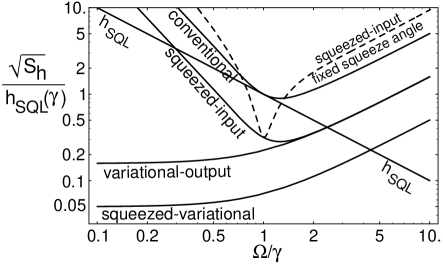
FIG. 4.: The square root of the spectral density $\sqrt{S_{h}}$ of the gravitational-wave noise for several interferometer designs, as a function of angular frequency $\Omega$, with optical losses assumed negligible; $\sqrt{S_{h}}$ is measured in units of the standard quantum limit at frequency $\Omega=\gamma$, and $\Omega$ is measured in units of $\gamma$. The noise curves shown are: (i) the standard quantum limit itself, $h_{\rm SQL}(\Omega)$ [Eq. (27)]; (ii) the noise for a conventional interferometer with laser power $I_{o}=I_{\rm SQL}$ [Eq. (36)]; (iii) the noise for a squeezed-input interferometer with $I_{o}=I_{\rm SQL}$, squeeze factor $e^{-2R}=0.1$, and (a) optimized FD squeeze angle $\lambda=-\Phi(\Omega)$ [Eq. (62); solid curve], (b) optimized frequency-independent squeeze angle [Eq. (67); dashed curve]; (iv) the noise for a variational-output interferometer with $I_{o}=10I_{\rm SQL}$ and optimized frequency-dependent homodyne phase $\zeta=\Phi(\Omega)$ [Eq. (73)]; and (v) the noise for a squeezed-variational interferometer with $I_{o}=10I_{\rm SQL}$, input squeeze factor $e^{-2R}=0.1$, and optimized input squeeze angle $\lambda=\pi/2$ and output homodyne phase $\zeta=\Phi(\Omega)$ [Eq. (92)].

IV Strategies to Beat the SQL, and Their Lossless Performance

A Motivation: Ponderomotive squeezing

The interferometer’s input-output relations $\Delta b_{1}=a_{1}e^{2i\beta}$, $\Delta b_{2}=(a_{2}-{\cal K}a_{1})e^{2i\beta}$ can be regarded as consisting of the uninteresting phase shift $e^{2i\beta}$, and a rotation in the $\{a_{1},a_{2}\}$ plane (i.e., $\{\cos\omega_{o}t,\sin\omega_{o}t\}$ plane), followed by a squeeze:

$$b_{j}=S^{{\dagger}}(r,\phi)R^{{\dagger}}(-\theta)a_{j}e^{2i\beta}R(-\theta)S(r,\phi)\;.$$ (37)

Here $R(-\theta)$ is the rotation operator and $S(r,\phi)$ the squeeze operator for two-photon quantum optics; see Appendix A for a very brief summary, and Refs. [26, 27] for extensive detail. The rotation angle $\theta$, squeeze angle $\phi$ and squeeze factor $r$ are given by

$$\theta=\arctan({\cal K}/2),\;\;\phi={1\over 2}{\rm arccot}({\cal K}/2),\;\;r={\rm arcshinh}({\cal K}/2).$$ (38)

Note that, because the coupling constant $\cal K$ depends on frequency $\Omega$ [Eq. (25)], the rotation angle, squeeze angle, and squeeze factor are frequency dependent. This frequency dependence will have major consequences for the QND interferometer designs discussed below.

The rotate-and-squeeze transformation (37) for the two-photon amplitudes implies corresponding rotate-and-squeeze relations for the one-photon creation and annihilation operators

$$b_{\pm}=S^{{\dagger}}(r,\phi)R^{{\dagger}}(-\theta)a_{\pm}e^{\pm 2i\beta}R(-\theta)S(r,\phi)\;.$$ (39)

Denote by $|0_{a_{+}}\rangle$ the vacuum for the in mode at frequency $\omega_{o}+\Omega$, by $|0_{a_{-}}\rangle$ that for the in mode at $\omega_{o}-\Omega$, and by $|0_{a_{\pm}}\rangle$ the vacuum for one or the other of these modes; and denote similarly the vacuua for the out modes, $|0_{b\pm}\rangle$. Then $|0_{a_{\pm}}\rangle$ is the state annihilated by $a_{\pm}$ and $|0_{b_{\pm}}\rangle$ is that annihilated by $b_{\pm}$. Correspondingly, the rotate-squeeze relation (39) implies that

$$b_{\pm}|0_{b_{\pm}}\rangle=S^{{\dagger}}R^{{\dagger}}a_{\pm}e^{\pm 2i\beta}RS|0_{b_{\pm}}\rangle=0\;,$$ (40)

where the parameters of the squeeze and rotation operators are those given in Eqs. (38) and (39). This equation implies that $e^{\pm 2i\beta}RS|0_{b_{\pm}}\rangle$ is annihilated by $a_{\pm}$ and therefore is the in vacuum $|0_{a_{\pm}}\rangle$ for the in mode $\omega_{o}\pm\Omega$:

$$e^{\pm 2i\beta}RS|0_{b_{\pm}}\rangle=|0_{a_{\pm}}\rangle\;.$$ (41)

Applying $R^{{\dagger}}$ and noting that $R^{{\dagger}}|0_{a_{\pm}}\rangle=|0_{a_{\pm}}\rangle$ (the vacuum is rotation invariant), we obtain

$$|0_{a_{\pm}}\rangle=e^{\pm 2i\beta}S(r,\phi)|0_{b_{\pm}}\rangle\;.$$ (42)

Thus, the in vacuum is equal to a squeezed out vacuum, aside from an uninteresting, frequency-dependent phase shift. The meaning of this statement in the context of a conventional interferometer is the following:

For a conventional interferometer, the in state is

$$|{\rm in}\rangle=|0_{a_{\pm}}\rangle=e^{\pm 2i\beta}S(r,\phi)|0_{b_{\pm}}\rangle\;;$$ (43)

and because we are using the Heisenberg Picture where the state does not evolve, the light emerges from the interferometer in this state. However, in passing through the interferometer, the light’s quadrature amplitudes evolve from $a_{j}$ to $b_{j}$. Correspondingly, at the output we should discuss the properties of the unchanged state in terms of a basis built from the out vacuum $|0_{b_{\pm}}\rangle$. Equation (42) says that in this out language, the light has been squeezed at the angle $\phi$ and squeeze-factor $r$ given by Eq. (38). This squeezing is produced by the back-action force of fluctuating radiation pressure on the test masses. That back action has the character of a ponderomotive nonlinearity first recognized by Braginsky and Manukin [15]. The correlations inherent in this squeezing form the foundation for the QND interferometers discussed below.

One can also deduce this ponderomotive squeezing from the in-out relations $\Delta b_{1}=a_{1}e^{2i\beta}$, $\Delta b_{2}=(a_{2}-{\cal K}a_{1})e^{2i\beta}$ [Eq. (23)], the expressions

$${1\over 2}2\pi\delta(\Omega-\Omega^{\prime})S_{b_{j}}(f) = \langle{\rm in}|\Delta b_{j}\Delta{b_{j^{\prime}}}^{{\dagger}}|{\rm in}\rangle_{\rm sym}\;,$$ (44)

$${1\over 2}2\pi\delta(\Omega-\Omega^{\prime})S_{b_{1}b_{2}}(f) = \langle{\rm in}|{1\over 2}(\Delta b_{1}\Delta{b_{2^{\prime}}}^{{\dagger}}+\Delta b_{1}^{\rm{\dagger}}\Delta b_{2^{\prime}})|{\rm in}\rangle_{\rm sym}$$ (45)

for the spectral densities and cross spectral densities of $b_{1}$ and $b_{2}$, and the spectral densities $S_{a_{1}}=S_{a_{2}}=1$, $S_{a_{1}a_{2}}=0$ [Eqs. (33)]. These imply that for a conventional interferometer

$$S_{b_{1}}=1\;,\quad S_{b_{2}}=1+{\cal K}^{2}\;,\quad S_{b_{1}b_{2}}=-{\cal K}\;.$$ (47)

Rotating $\Delta b_{j}$ through the angle $\phi={1\over 2}{\rm arccot}({\cal K}/2)$ to obtain

$$b^{\prime}_{1}=b_{1}\cos\phi+b_{2}\sin\phi\;,\quad b^{\prime}_{2}=b_{2}\cos\phi-b_{1}\sin\phi\;,$$ (48)

and using Eqs. (LABEL:Sb1b2Def) and (47), we obtain

$$S_{b^{\prime}_{1}} = e^{-2r}=\left(\sqrt{1+({\cal K}/2)^{2}}-{\cal K}/2\right)^{2}\simeq 1/{\cal K}\hbox{ if }{\cal K}\gg 1\;,$$ (49)

$$S_{b^{\prime}_{2}} = e^{+2r}=\left(\sqrt{1+({\cal K}/2)^{2}}+{\cal K}/2\right)^{2}\;,\quad S_{b^{\prime}_{1}b^{\prime}_{2}}=0\;,$$ (50)

which represents a squeezing of the input vacuum noise in the manner described formally by Eqs. (43) and (38).

This ponderomotive squeezing is depicted by the noise ellipse of Fig. 5. For a conventional interferometer ($b_{2}$ measured via photodetection), the signal is the arrow along the $b_{2}$ axis, and the square root of the noise spectral density $S_{b_{2}}$ is the projection of the noise ellipse onto the $b_{2}$ axis. For a detailed discussion of this type of graphical representation of noise in two-photon quantum optics see, e.g., Ref. [26].

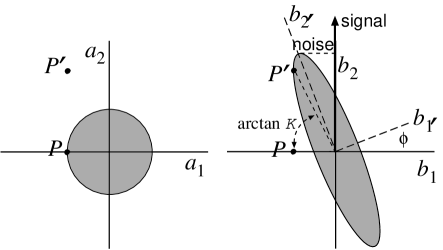
FIG. 5.: Noise ellipses for a conventional interferometer. Left: Noise for vacuum that enters the interferometer’s dark port. Right: Noise for ponderomotively squeezed vacuum that exits at the dark port along with the gravitational-wave signal; the ponderomotive squeeze has moved the point $P$ to the new point $P^{\prime}$ [$b_{1}=a_{1}$, $b_{2}=a_{2}-{\cal K}a_{1}$, Eqs. (23)]. These noise ellipses have dimensions and shapes described by the noise spectral densities (33), (47) and (LABEL:Sb1'b2'), and by the squeeze equations (43) and (38). The minor radius of the output noise ellipse is $\sqrt{S_{b^{\prime}_{1}}}=e^{-r}$, and its major radius is $\sqrt{S_{b^{\prime}_{2}}}=e^{+r}$, where $r$ is the squeeze factor; cf. Eqs. (38) and (LABEL:Sb1'b2'). The conventional interferometer measures $b_{2}$, which contains the indicated noise [cf. Eq. (30)] and the indicated signal [$\delta b_{2}=\sqrt{2{\cal K}}h/h_{\rm SQL}$; cf. Eq. (23)]. For a detailed discussion of noise ellipses in 2-photon quantum optics see, e.g., Ref. [26].

B Squeezed-Input Interferometer

Interferometer designs that can beat the SQL (35) are sometimes called “QND interferometers”. Unruh [14] has devised a QND interferometer design based on (i) putting the input electromagnetic fluctuations at the dark port ($a_{1}$ and $a_{2}$) into a squeezed state, and (ii) using standard photodetection to measure the interferometer’s output field. We shall call this a squeezed-input interferometer. The squeezing of the input has been envisioned as achieved using nonlinear crystals [20, 21], but one might also use ponderomotive squeezing.

The squeezed-input interferometer is identical to the conventional interferometer of Sec. III, except for the choice of the in state $|{\rm in}\rangle$ for the dark-port field. Whereas a conventional interferometer has $|{\rm in}\rangle=|0_{a}\rangle$, the squeezed-input interferometer has

$$|{\rm in}\rangle=S(R,\lambda)|0_{a}\rangle\;,$$ (52)

where $R$ is the largest squeeze factor that the experimenters are able to achieve ($e^{-2R}\sim 0.1$ in the LIGO-III time frame), and $\lambda=\lambda(\Omega)$ is a squeeze angle that depends on side-band frequency. One adjusts $\lambda(\Omega)$ so as to minimize the noise in the output quadrature amplitude $b_{2}$, which (i) contains the gravitational-wave signal and (ii) is measured by standard photodetection.

The gravitational-wave noise for such an interferometer is proportional to

$$\langle{\rm in}|h_{n}h_{n^{\prime}}|{\rm in}\rangle=\langle 0_{a}|h_{ns}h_{ns^{\prime}}|0_{a}\rangle$$ (53)

[Eq. (29)], where $h_{ns}$ is the squeezed gravitational-wave noise operator

$$h_{ns}=S^{{\dagger}}(R,\lambda)h_{n}S(R,\lambda)$$ (54)

and $h_{n}^{\prime}\equiv h_{n}(\Omega^{\prime})$. By inserting expression (28) for $h_{n}$ into Eq. (54) and then combining the interferometer’s ponderomotive squeeze relation $\Delta b_{2}=(a_{2}-{\cal K}a_{1})e^{2i\beta}$ with the action of the squeeze operator on $a_{1}$ and $a_{2}$ [Eq. (A12)], we obtain

$$h_{ns}=-{h_{\rm SQL}\over\sqrt{2{\cal K}}}\sqrt{(1+{\cal K}^{2})}\;e^{i\beta}$$ (55)

$$\quad\times\left(a_{1}\{\cosh R\cos\Phi-\sinh R\cos[\Phi-2(\Phi+\lambda)]\}\right.$$ (56)

$$\quad\;\left.-a_{2}\{\cosh R\sin\Phi-\sinh R\sin[\Phi-2(\Phi+\lambda)]\}\right)\;,$$ (57)

where

$$\Phi\equiv{\rm arccot}{\cal K}\;.$$ (58)

We can read the spectral density of the gravitational-wave noise off of Eq. (57) by recalling that in the $|0_{a}\rangle$ vacuum state [which is relevant because of Eq. (53)], $a_{1}$ and $a_{2}$ can be regarded as random processes with spectral sensities $S_{a_{1}}=S_{a_{2}}=1$ and vanishing cross spectral density [Eqs. (33)]:

$$S_{h}={h_{\rm SQL}^{2}\over 2}\left({1\over{\cal K}}+{\cal K}\right)\Big{(}\cosh 2R-\cos[2(\lambda+\Phi)]\sinh 2R\Big{)}.$$ (59)

It is straightforward to verify that this noise is minimized by making it proportional to $\cosh 2R-\sinh 2R=e^{-2R}$, which is achieved by choosing for the input squeeze angle

$$\lambda(\Omega)=-\Phi(\Omega)\equiv-{\rm arccot}{\cal K}(\Omega)\;.$$ (60)

The result is

$$S_{h}={h_{\rm SQL}^{2}\over 2}\left({1\over{\cal K}}+{\cal K}\right)e^{-2R}\;.$$ (61)

This says that the squeezed-input interferometer has the same noise spectral density as the conventional interferometer, except for an overall reduction by $e^{-2R}$, where $R$ is the squeeze factor for the dark-port input field (a result deduced by Unruh [14] and later confirmed by Jaekel and Reynaud [18] using a different method); see Fig. 4. This result implies that the squeezed-input interferometer can beat the amplitude SQL by a factor $e^{-R}$.

When the laser power $I_{o}$ of the squeezed-input interferometer is optimized for detection at the frequency $\Omega=\gamma$ ($I_{o}=I_{\rm SQL}$ as for a conventional interferometer), the noise spectrum becomes

$$S_{h}={4\hbar\over mL^{2}\Omega^{2}}\left[{2\gamma^{4}\over\Omega^{2}(\gamma^{2}+\Omega^{2})}+{\Omega^{2}(\gamma^{2}+\Omega^{2})\over 2\gamma^{4}}\right]e^{-2R}\;.$$ (62)

This optimized noise is shown in Fig. 4 for $e^{-2R}=0.1$, along with the noise spectra for other optimized interferometer designs.

In previous discussions of this squeezed-input scheme [14, 18, 19], no attention has been paid to the practical problem of how to produce the necessary frequency dependence

$$\lambda(\Omega)=-\Phi(\Omega)=-{\rm arccot}{2\gamma^{4}\over\Omega^{2}(\gamma^{2}+\Omega^{2})}$$ (63)

of the squeeze angle. In Sec. V C, we shall show that this $\lambda(\Omega)$ can be achieved by squeezing at a frequency-independent squeeze angle (using, e.g., a nonlinear crystal for which the squeeze angle will be essentially frequency-independent because the gravity-wave bandwidth, $<1000$ Hz, is so small compared to usual optical bandwidths ) and then filtering through two Fabry-Perot cavities. This squeezing and filtering must be performed before injection into the interferometer’s dark port; see Fig. 1 for a schematic diagram.

The signal and noise for this squeezed-input interferometer are depicted in Fig. 6.

We comment, in passing, on two other variants of a squeezed-input interferometer:

(i) If, for some reason, the filter cavities cannot be implemented successfully, one can still inject squeezed vacuum at the dark port with a frequency-independent phase that is optimized for the lowest point in the noise curve, $\Omega=\gamma$; i.e. (with the input power optimized to $I_{o}=I_{\rm SQL}$):

$$\lambda=-\Phi(\gamma)=-\pi/4\;;$$ (64)

cf.  Eq. (63). In this case the noise spectrum is

$$S_{h}={h_{\rm SQL}^{2}\over 2}\left({1\over{\cal K}}+{\cal K}\right)$$ (65)

$$\quad\times\left[(\cosh R\cos\Phi-\sinh R\sin\Phi)^{2}\right.$$ (66)

$$\quad\;\left.+(\cosh R\sin\Phi-\sinh R\cos\Phi)^{2}\right]\;;$$ (67)

[Eq. (59), translated into gravitational-wave noise via Eq. (30)]. This noise spectrum is shown as a dashed curve in Fig. 4, for $e^{-2R}=0.1$. The SQL is beat by the same factor $\mu=\sqrt{e^{-2R}}\simeq 0.32$ as in the case of a fully optimized squeezed-input interferometer, but the frequency band over which the SQL is beat is significantly smaller than in the optimized case, and the noise is worse than for a conventional interferometer outside that band.

(ii) Caves [17], in a paper that preceeded Unruh’s and formed a foundation for Unruh’s ideas, proposed a squeezed-input interferometer with the squeeze angle set to $\lambda=\pi/2$ independent of frequency. In this case, Eq. (59), translated into gravitational-wave noise via Eq. (30), says that

$$S_{h}={h_{\rm SQL}^{2}\over 2}\left({1\over{e^{2R}\cal K}}+e^{2R}{\cal K}\right)\;.$$ (68)

Since $\cal K$ is proportional to the input laser power $I_{o}$, Caves’ interferometer produces the same noise spectral density as a conventional interferometer [Eq. (34)] but with an input power that is reduced by a factor $e^{-2R}$. This is a well-known result.

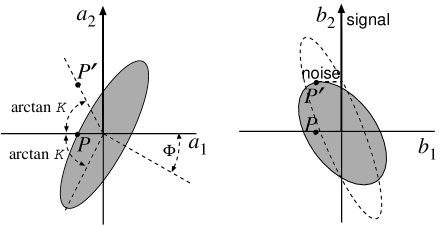
FIG. 6.: Noise ellipses for a squeezed-input interferometer. Left: Noise for squeezed vacuum that enters the interferometer’s dark port. The field is squeezed at the angle $\lambda=-\Phi$. Right: Noise for the field that exits at the dark port along with the gravitational-wave signal. This output field results from the interferometer’s ponderomotive squeezing of the input field [e.g., point $P$ goes to point $P^{\prime}$ in accord with $b_{1}=a_{1}$, $b_{2}=a_{2}-{\cal K}a_{1}$; Eqs. (23)]. If the input field had been vacuum as in a conventional interferometer [Fig. 5], then the output would have been squeezed in the manner of the dashed ellipse. The two squeezes (input and ponderomotive) result in the shaded ellipse, whose projection along the axis measured by the photodetector ($b_{2}$ axis) has been minimized by the choice of squeeze angle, $\lambda=-\Phi$.

C Variational-output interferometer

Vyatchanin, Matsko and Zubova [23, 24, 25] have devised a QND interferometer design based on (i) leaving the dark-port input field in its vacuum state, $|{\rm in}\rangle=|0_{a}\rangle$, and (ii) changing the output measurement from standard photodetection (measurement of $b_{2}$) to homodyne detection at an appropriate, frequency-dependent (FD) homodyne phase $\zeta(\Omega)$ – i.e., measurement of

$$b_{\zeta}=b_{1}\cos\zeta+b_{2}\sin\zeta\;.$$ (69)

In their explorations of this idea, Vyatchanin, Matsko and Zubova [23, 24, 25] did not identify any practical scheme for achieving such a FD homodyne measurement, so they approximated it by homodyne detection with a homodyne phase that depends on time rather than frequency — a technique that they call a “quantum variational measurement”.

In Sec. V below, we show that the optimized FD homodyne measurement can, in fact, be achieved by filtering the interferometer output through two Fabry-Perot cavities and then performing standard, balanced homodyne detection at a frequency-independent homodyne phase; see Fig. 2 for a schematic diagram. We shall call such an scheme a variational-output interferometer. The word “variational” refers to (i) the fact that the measurement entails monitoring a frequency-varying quadrature of the output field, as well as (ii) the fact that the goal is to measure variations of the classical force acting on the interferometer’s test mass (the original Vyatchanin-Matsko-Zubova motivation for the word).

The monitored FD amplitude $b_{\zeta}$ [Eq. (69)] can be expressed in terms of the interferometer’s dark-port input amplitudes $a_{1}$, $a_{2}$ and the Fourier transform of the gravitational-wave field $h$ as

$$b_{\zeta}=\sin\zeta\left(\sqrt{2{\cal K}}{h\over h_{\rm SQL}}e^{i\beta}+[a_{2}+(\cot\zeta-{\cal K})a_{1}]e^{2i\beta}\right)\;;$$ (70)

cf. Eqs. (23) and (69). Correspondingly, the operator describing the Fourier transform of the interferometer’s gravitational-wave noise is

$$h_{n}(\Omega)={h_{\rm SQL}\over\sqrt{2{\cal K}}}e^{i\beta}[a_{2}+a_{1}(\cot\zeta-{\cal K})]\;;$$ (71)

cf. Eq. (30).

The radiation-pressure-induced back action of the measurement on the interferometer’s test masses is embodied in the $-{\cal K}a_{1}$ term of this equation; cf. Eq. (23) and subsequent discussion. It should be evident that by choosing

$$\zeta=\Phi\equiv{\rm arccot}{\cal K}\;,$$ (72)

we can completely remove the back-action noise from the measured interferometer output; cf. Fig. 7. This optimal choice of the FD homodyne phase, together with the fact that the input state is vacuum, $|{\rm in}\rangle=|0_{a}\rangle$, leads to the gravitational-wave noise

$$S_{h}={h^{2}_{\rm SQL}\over 2}{1\over{\cal K}}={1\over I_{o}/I_{\rm SQL}}\left({4\hbar\over mL^{2}\Omega^{2}}\right){\Omega^{2}(\gamma^{2}+\Omega^{2})\over 2\gamma^{4}}\;.$$ (73)

cf. Eqs. (29) and (32).

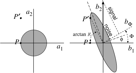
FIG. 7.: Noise ellipses for a variational-output interferometer. Left: Noise for the ordinary vacuum that enters the interferometer’s dark port. Right: Noise for the field that exits at the dark port along with the gravitational-wave signal. These noise ellipses are the same as for a conventional interferometer, Fig. 5, but here the quantity measured is the quadrature amplitude $b_{\Phi}$ with frequency dependent phase $\Phi\equiv{\rm arccot}{\cal K}$. It is informative to compare the measured phase $\Phi$ with the angle of ponderomotive squeeze $\phi={1\over 2}{\rm arccot}({\cal K}/2)$. They are related by $\tan\Phi={1\over 2}\tan 2\phi=\tan\phi/(1-\tan^{2}\phi)$, so $\Phi$ is always larger than $\phi$; but for large ${\cal K}$ (strong beating of the SQL), they become small and nearly equal.

This noise for an optimized variational-output interferometer is entirely due to shot noise of the measured light, and continues to improve $\propto 1/I_{o}$ even when the input light power $I_{o}$ exceeds $I_{\rm SQL}$. Figure 4 shows this noise, along with the noise spectra for other optimized interferometer designs.

It is interesting that the optimal frequency-dependent homodyne phase $\Phi$ for this variational-output interferometer is the same, aside from sign, as the optimal frequency-dependent squeeze angle for the squeezed-input interferometer; cf. Eq. (60).

D Comparison of squeezed-input and variational-output interferometers

The squeezed-input and variational-output interferometers described above are rather idealized, most especially because they assume perfect, lossless optics. When we relax that assumption in Sec. VI below, we shall see that, for realistic squeeze factors $e^{-2R}$ and losses $\epsilon_{*}$, the two interferometers have essentially the same performance, but the variational-output intefermometer requires $\sim 10$ times higher input power $I_{o}$. In this section we shall seek insight into the physics of these interferometers by comparing them in the idealized, lossless limit.

Various comparisons are possible. The noise curves in Fig. 4 illustrate one comparison: When the FD homodyne angle has been optimized, a lossless variational-output interferometer reduces shot noise below the SQL and completely removes back-action noise; by contrast, when the FD squeeze angle has been optimized, a squeezed-input interferometer reduces shot noise and reduces but does not remove back-action noise; cf. Eqs. (73) and (61).

In variational-output interferometers, after optimizing the FD homodyne angle, the experimenter has further control of just one input/output parameter: the laser intensity or equivalently $I_{o}/I_{\rm SQL}={\cal K}(\Omega=\gamma)$. When $I_{o}/I_{\rm SQL}$ is increased, the shot noise decreases; independent of its value, the back-action noise has already been removed completely; cf. Eq. (73). By contrast, in squeezed-input interferometers, after optimizing the FD squeeze phase, the experimenter has control of two parameters: $I_{o}/I_{\rm SQL}$, which moves the minimum of the noise curve back and forth in frequency but does not lower its minimum [17], and the squeeze factor $R$, which reduces the noise by $e^{-2R}$; cf. Eq. (61).

Present technology requires that $R$ be approximately constant over the LIGO frequency band. However, in the same spirit as our assumption that the FD homodyne phase can be optimized at all frequencies, it is instructive to ask what can be achieved with an unconstrained, frequency-dependent (FD) squeeze factor $R(\Omega)$, when coupled to an unconstrained FD squeeze angle $\lambda(\Omega)$.

One instructive choice is $\lambda=-\hbox{arccot}{\cal K}$ as in our previous, optimized interferometer [Eq. (60)], and $e^{-2R}=1/(1+{\cal K}^{2})$. In this case, the squeezed-input interferometer has precisely the same noise spectrum as the lossless variational-output interferometer

$$S_{h}={h_{\rm SQL}^{2}\over 2{\cal K}}\;;$$ (74)

[Eq. (73)], and achieves it with precisely the same laser power.

Another instructive choice is an input squeeze that is inverse to the interferometer’s ponderomotive squeeze (a configuration we shall call “inversely input squeezed” or IIS): Let the dark-port input field before squeezing be described by annihilation operators $c_{\pm}$, so

$$c_{\pm}|{\rm in}\rangle=0\;,$$ (75)

i.e. the pre-squeeze field is vacuum. Then, denoting by $c_{1}$, $c_{2}$ the quadrature amplitudes of this pre-squeeze field, the IIS input squeezing is

$$a_{1}=c_{1}\;,\quad a_{2}=c_{2}+{\cal K}c_{1}\;,$$ (76)

where ${\cal K}(\Omega)$ is the interferometer’s frequency-dependent coupling constant (25). The interferometer’s ponderomotively squeezed output noise is then

$$\Delta b_{1}=a_{1}e^{2i\beta}=c_{1}e^{2i\beta}\;,\quad\Delta b_{2}=(a_{2}-{\cal K}a_{1})e^{2i\beta}=c_{1}e^{2i\beta}$$ (77)

[cf. Eq. (23)], i.e., the noise of the output light is that of the vacuum with a phase shift, but since the vacuum state is insensitive to phase, it is actually just the noise of the vacuum.

Figure 8 illustrates this: The IIS input light is squeezed in a manner that gets perfectly undone by the ponderomotive squeeze, so the output light has no squeeze at all. The fact that the input squeeze is inverse to the ponderomotive squeeze shows up in this diagram as an input noise ellipse that is the same as the output ellipse of the ponderomotively squeezed vacuum, Fig. 5, except for a reflection in the horizontal axis.

FIG. 8.: Noise ellipses for a squeezed-input interferometer whose input squeeze is inverse to the interferometer’s ponderomotive squeeze (“IIS interferomter”).

Because the output of the IIS interferometer is $b_{2}$ (ordinary photodetection) and the output light’s state is the ordinary vacuum, its gravitational-wave noise is

$$S_{h}={h_{\rm SQL}^{2}\over 2{\cal K}}\;;$$ (78)

cf. Eqs. (30), (29) and (33) (with $a_{j}$ replaced by $b_{j}$). Notice that this is identically the same noise spectral density as for our previous example [Eq. (74)] and as for a variational-output interferometer, and it is achieved in all three cases with the same light power.

The fact that our two squeezed-input examples produce the same noise spectrum using different squeeze angles and squeeze factors should not be surprising. The noise spectrum is a single function of $\Omega$ and it is being shaped jointly by the two squeeze functions $\lambda(\Omega)$ and $R(\Omega)$.

The fact that the IIS interferometer and the variational output interferometer produce the same noise spectra results from a reciprocity between the IIS and the variational-output configurations: The IIS interferometer has its input squeezed at the angle $-\Phi=-{\rm arccot}{\cal K}$ and it has vacuum-noise output, whereas the variational-output interferometer has vacuum-noise input and is measured at the homodyne angle $+\Phi=+{\rm arccot}{\cal K}$.

Note that the IIS interferometer has a different input squeeze angle [$\lambda=-{1\over 2}{\rm arccot}({\cal K}/2)$; cf. Eq. (38)] from that of the angle-optimized squeezed-input interferometer of Sec. IV B [$\lambda=-{\rm arccot}{\cal K}$; cf. Eq. (60)]. This difference shows clearly in the noise ellipses of Fig. 8 (the IIS interferometer) and Fig. 6 (the angle-optimized interferomter). Meoreover, this difference implies that by optimizing the IIS interferometer’s squeeze angle (changing it to $\lambda=-{\rm arccot}{\cal K}$), while keeping its squeeze factor unchanged [$R={\rm arcshinh}({\cal K}/2)$; cf. Eq. (38)], we can improve its noise performanance slightly. The improvement is from (78) to

$$S_{h}={h^{2}_{\rm SQL}\over 2{\cal K}}\left[{1+{\cal K}^{2}\over 1+{1\over 2}\left({\cal K}^{2}+{\cal K}\sqrt{{\cal K}^{2}+4}\right)}\right]$$ (79)

[which can be derived by setting $\lambda=-\Phi=-{\rm arccot}{\cal K}$ and $R={\rm arcshinh}({\cal K}/2)$ in Eq. (59), or by inserting $R={\rm arcshinh}({\cal K}/2)$ into Eq. (61)—note that (61) is valid for any angle-optimized, squeezed-input interferometer but not for the IIS interferometer]. The improvement factor in square brackets is quite modest; it lies between 0.889 and unity.

We reiterate, however, that the above comparison of interferometer designs is of pedagogical interest only. In the real world, the noise of a QND interferometer is strongly influenced by losses, which we consider in Sec. VI below.

E Squeezed-variational interferometer

The squeezed-input and variational-output techniques are complementary. By combining them, one can beat the SQL more strongly than using either one alone. We call an interferometer that uses the two techiques simultaneously a squeezed-variational interferometer.

The dark-port input of such an interferometer is squeezed by the maximum achievable squeeze factor $R$ at a (possibly frequency dependent) squeeze angle $\lambda(\Omega)$, so

$$|{\rm in}\rangle=S(R,\lambda)|0_{a}\rangle\;.$$ (80)

The dark-port output is subjected to FD homodyne detection with (possibly frequency dependent) homodyne angle $\zeta(\Omega)$; i.e., the measured quantity is the same output quadrature as for a variational-output interferometer, $b_{\zeta}$ [Eq. (70)], so the gravitational-wave noise operator is also the same

$$h_{n}(\Omega)={h_{\rm SQL}\over\sqrt{2{\cal K}}}\;e^{i\beta}\;[a_{2}+a_{1}(\cot\zeta-{\cal K})]e^{i\beta}$$ (81)

[Eq. (71)].

As for a squeezed-input interferometer, the gravitational-wave noise is proportional to

$$\langle{\rm in}|h_{n}h_{n^{\prime}}|{\rm in}\rangle=\langle 0_{a}|h_{ns}h_{ns^{\prime}}|0_{a}\rangle$$ (82)

[Eq. (29)], where $h_{ns}$ is the squeezed gravitational-wave noise operator

$$h_{ns}=S^{{\dagger}}(R,\lambda)h_{n}S(R,\lambda)\;.$$ (83)

By inserting expression (81) for $h_{n}$ into Eq. (83) and invoking the action of the squeeze operator on $a_{1}$ and $a_{2}$ [Eq. (A12)], we obtain

$$h_{ns}=-{h_{\rm SQL}\over\sqrt{2{\cal K}}}\sqrt{1+\tilde{\cal K}^{2}}\;e^{i\beta}$$ (84)

$$\quad\times\left(a_{1}\{\cosh R\cos\tilde{\Phi}-\sinh R\cos[\tilde{\Phi}-2(\tilde{\Phi}+\lambda)]\}\right.$$ (85)

$$\quad\;\left.-a_{2}\{\cosh R\sin\tilde{\Phi}-\sinh R\sin[\tilde{\Phi}-2(\tilde{\Phi}+\lambda)]\}\right)\;,$$ (86)

where

$$\tilde{\cal K}={\cal K}-\cot\zeta\;,\quad\tilde{\Phi}={\rm arccot\tilde{\cal K}}\;.$$ (87)

As for a squeezed-input interferometer [see passage following Eq. (58)], we can read the gravitational-wave spectral density off of Eq. (86) by regarding $a_{1}$ and $a_{2}$ as random processes with unit spectral densities and vanishing cross spectral density. The result is

$$S_{h} = {h_{\rm SQL}^{2}\over 2{\cal K}}(1+\tilde{\cal K}^{2})$$ (89)

$$\times\left\{e^{-2R}+\sinh 2R[1-\cos 2(\tilde{\Phi}+\lambda)]\right\}\;.$$

This noise is minimized by setting the input squeeze angle $\lambda$ and output homodyne phase $\zeta$ to

$$\lambda=\pi/2\;,\quad\zeta=\Phi={\rm arccot}{\cal K}\;,$$ (90)

which produces $\tilde{\cal K}=0$ and $\lambda=\tilde{\Phi}=\pi/2$, so

$$S_{h} = {h_{\rm SQL}^{2}\over 2{\cal K}}e^{-2R}$$ (91)

$$= {e^{-2R}\over I_{o}/I_{\rm SQL}}\left({4\hbar\over mL^{2}\Omega^{2}}\right){\Omega^{2}(\gamma^{2}+\Omega^{2})\over 2\gamma^{4}}\;;$$ (92)

see Fig. 4

Equation (90) says that, to optimize the (lossless) squeezed-variational interferometer, one should squeeze the dark-port input field at the frequency-independent squeeze angle $\zeta=\pi/2$ (which ends up squeezing the interferometer’s shot noise), and measure the output field at the same FD homodyne phase $\zeta=\Phi$ as for a variational-output interferometer; see Fig. 9. Doing so produces an output, Eq. (92), in which the radiation-pressure-induced back-action noise has been completely removed, and the shot noise has been reduced by the input squeeze factor $e^{-2R}$.

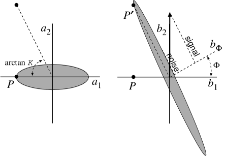
FIG. 9.: Noise ellipses for a squeezed-variational interferometer. Left: Noise for the squeezed vacuum that enters the interferometer’s dark port. Right: Noise for the field that exits at the dark port along with the gravitational-wave signal.

Because the optimal input squeeze angle is frequency independent, the squeezed variational interferometer needs no filter cavities on the input. However, they are needed on the output to enable FD homodyne detection; see Fig. 2 for a schematic diagram.

V FD Homodyne Detection and Squeezing

Each of the QND schemes discussed above requires homodyne detection with a frequency-dependent phase (FD homodyne detection) and/or input squeezed vacuum with a frequency-dependent squeeze angle (FD squeezed vacuum). In this section we sketch how such FD homodyne detection and squeezing can be achieved.

A General Method for FD Homodyne Detection

The goal of FD Homodyne Detection is to measure the electric-field quadrature

$$E_{\zeta}(t)=\sqrt{4\pi\hbar\omega_{o}\over{\cal A}c}\int_{0}^{\infty}\left(b_{\zeta}e^{-i\Omega t}+b_{\zeta}^{{\dagger}}e^{+i\Omega t}\right){d\Omega\over 2\pi}\;,$$ (93)

for which the quadrature amplitude is

$$b_{\zeta}=b_{1}\cos\zeta+b_{2}\sin\zeta\;,\quad\zeta=\zeta(\Omega)\;;$$ (94)

cf. Eqs. (16) and (69). If $\zeta$ were frequency independent, the measurement could be made by conventional balanced homodyne detection, with homodyne phase $\zeta$. In this subsection we shall show that, when $\zeta$ depends on frequency, the measurement can be achieved in two steps: first send the light through an appropriate filter (assumed to be lossless), and then perform conventional balanced homodyne detection.

The filter puts onto the light a phase shift $\alpha$ that depends on frequency. Let the phase shift be $\alpha_{+}$ for light frequency $\omega_{o}+\Omega$, and $\alpha_{-}$ for $\omega_{0}-\Omega$. The input to the filter has amplitudes (annihilation operators) $b_{\pm}$ at these two sidebands, and the filter output has amplitudes (denoted by a tilde)

$$\tilde{b}_{\pm}=b_{\pm}e^{i\alpha_{\pm}}\;.$$ (95)

The corresponding quadrature amplitudes are

$$b_{1}={b_{+}+b_{-}^{{\dagger}}\over\sqrt{2}}\;,\quad b_{2}={b_{+}-b_{-}^{{\dagger}}\over\sqrt{2}i}$$ (96)

at the input [Eqs. (6)], and the analogous expression with tildes at the output. Combining Eqs. (96) with and without tildes, and Eq. (95), we obtain for the output quadrature amplitudes in terms of the input

$$\tilde{b}_{1} = e^{i\alpha_{\rm m}}(b_{1}\cos\alpha_{\rm p}-b_{2}\sin\alpha_{\rm p})\;,$$ (97)

$$\tilde{b}_{2} = e^{i\alpha_{\rm m}}(b_{2}\cos\alpha_{\rm p}+b_{2}\sin\alpha_{\rm p})\;.$$ (98)

Here

$$\alpha_{\rm m}={1\over 2}(\alpha_{+}-\alpha_{-})\;,\quad\alpha_{\rm p}={1\over 2}(\alpha_{+}+\alpha_{-})\;.$$ (99)

The light with the output amplitudes $\tilde{b}_{1}$, $\tilde{b}_{2}$ is then subjected to conventional balanced homodyne detection with frequency-independent homodyne angle $\theta$, which measures an electric-field quadrature with amplitude

$$\tilde{b}_{\theta} = \tilde{b}_{1}\cos\theta+\tilde{b}_{2}\sin\theta$$ (100)

$$= e^{i\alpha_{\rm m}}[b_{1}\cos(\theta-\alpha_{\rm p})+b_{2}\sin(\theta-\alpha_{\rm p})]\;.$$ (101)

If we adjust the filter and the constant homodyne phase so that

$$\theta-\alpha_{\rm p}\equiv\theta-{1\over 2}(\alpha_{+}+\alpha_{-})=\zeta(\Omega)\;,$$ (102)

then, aside from the frequency-dependent phase shift $\alpha_{\rm m}$, the output quadrature amplitude will be equal to our desired FD amplitude:

$$\tilde{b}_{\theta}=e^{i\alpha_{\rm m}}b_{\zeta}\;.$$ (103)

The phase shift $\alpha_{\rm m}(\Omega)$ is actually unimportant; it can be removed from the signal in the data analysis (as can be the phase shift $\beta(\Omega)$ produced by the interferometer’s arm cavities).

To recapituate: FD homodyne detection with homodyne phase $\zeta(\Omega)$ can be achieved by filtering and conventional homodyne detection, with the filter’s phase shifts $\alpha_{\pm}$ (at $\omega=\omega_{o}\pm\Omega$) and the constant homodyne phase $\theta$ adjusted to satisfy Eq. (102).

B Realization of the filter

The desired FD homodyne phase is

$$\zeta=\Phi(\Omega)={\rm arccot}{\cal K} = {\rm arccot}\left({\Lambda^{4}\over\Omega^{2}(\gamma^{2}+\Omega^{2})}\right)$$ (104)

$$= {\rm arctan}\left(\Omega^{2}(\gamma^{2}+\Omega^{2})\over\Lambda^{4}\right)\;,$$ (105)

where

$$\Lambda^{4}=(I_{o}/I_{\rm SQL})2\gamma^{4}$$ (106)

[cf. Eqs. (25) and (58)]. Recall that $\gamma\simeq 2\pi\times 100$Hz is the optimal frequency of operation of the interferometer, and to beat the SQL by a moderate amount will require $I_{o}/I_{\rm SQL}\sim 10$ so $\Lambda^{4}\sim 20\gamma^{4}$, i.e., $\Lambda\sim 2\gamma$.

In Appendix C we show that this desired FD phase can be achieved by filtering the light with two successive lossless Fabry-Perot filter cavities, followed by conventional homodyne detection at homodyne angle

$$\theta=\pi/2$$ (107)

[i.e., homodyne measurement of $\tilde{b}_{2}$ at the filter output; cf. Eq. (101)]. The two filter cavities (denoted I and II) produce phase shifts $\alpha_{{\rm I}\pm}$ and $\alpha_{\rm II}\pm$ on the $\omega_{o}\pm\Omega$ side bands, so upon emerging from the second cavity, the net phase shifts are

$$\alpha_{\pm}=\alpha_{{\rm I}\pm}+\alpha_{{\rm II}\pm}\;.$$ (108)

Each cavity ($J=$I or II) is characterized by two parameters: its decay rate (bandwidth) $2\delta_{J}$ (with $J=\hbox{I or II}$), and its fractional resonant-frequency offset from the light’s carrier frequency $\omega_{o}$,

$$\xi_{J}\equiv{\omega_{o}-\omega_{{\rm res}\,J}\over\delta_{J}}\;.$$ (109)

Here $\omega_{{\rm res}\,J}$ is the resonant frequency of cavity $J$. In terms of these parameters, the phase shifts produced in the $\omega_{o}\pm\Omega$ side bands by cavity $J$ are

$$\alpha_{J\pm}={\rm arctan}(\xi_{J}\pm\Omega/\delta_{J})\;.$$ (110)

The filters’ parameters must be adjusted so that the net phase shift (108), together with the final homodyne angle $\theta=\pi/2$, produce the desired FD phase, Eqs. (102) and (105).

In Appendix C we derive the following values for the filter parameters $\xi_{\rm I}$, $\delta_{\rm I}$, $\xi_{\rm II}$ and $\delta_{\rm II}$ as functions of the parameters $\Lambda$ and $\gamma$ that appear in the desired FD homodyne phase. Define the following four functions of $\Lambda$ and $\gamma$

$$P \equiv {4\Lambda^{4}\over\gamma^{4}}\;,\quad Q\equiv{1+\sqrt{1+P^{2}}\over 2}\;,$$ (112)

$$A_{+} \equiv {Q+\sqrt{Q}\over P}\;,\quad A_{-}\equiv{Q-\sqrt{Q}\over P}\;.$$ (113)

Then in terms of these functions, the filter parameters are

$$\xi_{\rm I} = {1\over 2A_{+}}+\sqrt{1+{1\over(2A_{+})^{2}}}\;,$$ (114)

$$\xi_{\rm II} = {1\over 2A_{-}}-\sqrt{1+{1\over(2A_{-})^{2}}}\;,$$ (115)

$${\delta_{\rm I}\over\gamma} = \sqrt{P\over 8\xi_{\rm I}\sqrt{Q}}\;,$$ (116)

$${\delta_{\rm II}\over\gamma} = \sqrt{P\over 8(-\xi_{\rm II})\sqrt{Q}}\;.$$ (117)

Note that, when the cavity half-bandwidths $\delta_{J}$ are expressed in terms of the half-bandwidth $\gamma$ of the interferometer’s arm cavities, as in Eqs. (116) and (117), then the filter parameters depend on only one characteristic of the desired FD homodyne phase: the quantity $(\Lambda/\gamma)^{4}=2I_{o}/I_{\rm SQL}$. Figure 10 depicts the filter parameters as functions of this quantity.

FIG. 10.: The parameters characterizing the two Fabry-Perot cavities that are used, together with conventional homodyne detection at phase $\theta=\pi/2$, to produce FD homodyne detection at the desired frequency-dependent phase (105). The quantities $\xi_{\rm I}$ and $\xi_{\rm II}$ are the filters’ fractional frequency offsets from the light’s carrier frequency (109); $\delta_{\rm I}/\gamma$ and $\delta_{\rm II}/\gamma$ are the filters’ half bandwidths in units of the half-bandwidth of the interferometer’s identical arm cavities. The functional forms of these parameters are Eqs. (V B).

As Fig. 10 shows, the half-bandwidths of the two filter cavities are within a factor $\sim 2$ of that of the interferometer’s arm cavities. This is so for the entire range of laser powers, $I_{o}/I_{\rm SQL}$, that are likely to be used in QND interferometers, at least in the early years (e.g., LIGO-III; ca. 2008–2010). Moreover, the filter cavities’ fractional frequency offsets $\xi_{J}$ are of order unity ($-0.5<\xi_{J}\lesssim 2$). Thus, the desired properties of the filter cavities are not much different from those of the interferometer’s arm cavities.

In Sec. VI below, we shall see that the most serious limitation on the sensitivities of variational-output and squeezed-variational interferometers is optical loss in the filter cavities. To minimize losses, the cavities should be very long (so the cavities’ stored light encounters the mirrors a minimum number of times). This suggests placing the filter cavities in the interferometer’s 4km-long arms, alongside the interferometer’s arm cavities.

C Squeezing with frequency-dependent squeeze angle

Just as the variational-output and squeezed-variational interferometers require homodyne detection at a FD phase, so a squeezed-input interferometer requires squeezing at a FD angle $\lambda(\Omega)$.

The nonlinear-optics techniques currently used for squeezing will produce a squeeze angle that is nearly constant over the very narrow frequency band of gravitational-wave interferometers, $|\omega-\omega_{o}|\lesssim\hbox{(a few)}\times\gamma\sim 10^{-12}\omega_{o}$. What we need is a way to change the squeeze angle from its constant nonlinear-optics-induced value to the desired frequency-dependent value, $\lambda=-\Phi(\Omega)$ [Eq. (63)].

Just as FD homodyne detection can be achieved by sending the light field through appropriate filters followed by a frequency-independent homodyne device, so also FD squeezing can be achieved by squeezing the input field in the standard frequency-independent way, and then sending it through appropriate filters. Moreover, since the necessary squeeze angle has the same frequency dependence $-\Phi(\Omega)$ as the homodyne phase (aside from sign), the filters needed in FD squeezing are nearly the same as those needed in FD homodyne detection: The filtering can be achieved by sending the squeezed input field through two Fabry-Perot cavities before injecting it into the interferometer, and the cavity parameters are given by formulae analogous to Eqs. (V B):

$$Q \equiv {1+\sqrt{65}\over 2}\;,\quad A_{\pm}\equiv-{Q\pm\sqrt{Q}\over 8}\;,$$ (119)

$$\xi_{\rm I} = {1\over 2A_{+}}-\sqrt{1+{1\over(2A_{+})^{2}}}\;,$$ (120)

$$\xi_{\rm II} = {1\over 2A_{-}}+\sqrt{1+{1\over(2A_{-})^{2}}}\;.$$ (121)

$${\delta_{\rm I}\over\gamma} = \sqrt{1\over(-\xi_{\rm I})\sqrt{Q}}\;,$$ (122)

$${\delta_{\rm II}\over\gamma} = \sqrt{1\over\xi_{\rm II}\sqrt{Q}}\;.$$ (123)

The details of the calculations are essentially the same as Appendix C, but with Eq. (C2) changed into the following expression for the initial frequency-independent squeeze angle $\theta$ and the cavities’ frequency-dependent phase shifts $\alpha_{J\pm}$:

$$\tan\Phi(\Omega) \equiv -{\Omega^{2}(\gamma^{2}+\Omega^{2})\over 2\gamma^{4}}$$ (124)

$$= \tan\left(\theta-{\alpha_{I+}+\alpha_{I-}+\alpha_{II+}+\alpha_{II-}\over 2}\right)\;.$$ (125)

VI Influence of Optical Losses on QND Interferometers

A The role of losses

It is well known that, when one is working with squeezed light, any source of optical loss (whether fundamentally irreversible or not) can debilitate the light’s squeezed state. This is because, wherever the squeezed light can leave one’s optical system, vacuum field can (and must) enter by the inverse route; and the entering vacuum field will generally be unsqueezed [31].

All of the QND interferometers discussed in this paper rely on squeezed-light correlations in order to beat the SQL — with the squeezing always produced ponderomotively inside the interferometer and, in some designs, also present in the dark-port input field. Thus, optical loss is a serious issue for all the QND interferometers.

In this section we shall study the influence of optical losses on the optimized sensitivities of our three types of QND interferometers.

B Sources of optical loss

The sources of optical loss in our interferometers are the following:

1. For light inside the interferometer’s arm cavities and inside the Fabry-Perot filter cavities: scattering and absorption on the mirrors and finite transmissivity through the end mirrors. We shall discuss these quantitatively at the end of the present subsection. (In addition, wave front errors and birefringence produced in the arm cavities and filters, e.g. via power-dependent changes in the shapes and optical properties of the mirrors, will produce mode miss-matching and thence losses in subsequent elements of the output optical train.)

2. For squeezed vacuum being injected into the interferometer: fractional photon losses $\epsilon_{\rm circ}$ in the circulator used to do the injection, in the beam splitter $\epsilon_{\rm bs}$, and in mode-matching into the interferometer $\epsilon_{\rm mm}$.

3. For the signal light traveling out of the interferometer: In addition to losses in the arm cavities and filter cavities, also fractional photon losses in the beam splitter $\epsilon_{\rm bs}$, in the circulator $\epsilon_{\rm circ}$, in mode-matching into each of the filter cavities $\epsilon_{\rm mm}$, in mode-matching with the local-oscillator light used in the homodyne detection $\epsilon_{\rm lo}$, and in the photodiode inefficiency $\epsilon_{\rm pd}$.

It is essential to pursue R&D with the aim of driving these fractional photon losses down to

$$\epsilon_{\rm circ}\sim\epsilon_{\rm bs}\sim\epsilon_{\rm mm}\sim\epsilon_{\rm lo}\sim\epsilon_{\rm pd}\sim 0.001\;.$$ (126)

These loss levels are certainly daunting. However, it is well to keep in mind that attaining the absolute lowest loss levels will likely be an essential component of any advanced interferometer that attempts to challenge and surpass the SQL. In the current case, discussions with Stan Whitcomb and the laboratory experience of one of the authors (HJK) lead us to suggest that it may be technically plausible to achieve the levels of Eq. (126) in the LIGO-III time frame, though a vigorous research effort will be needed to determine the actual feasibility.

These loss levels are certainly daunting, but based on discussions with Stan Whitcomb and on the laboratory experience of one of the authors (HJK), it seems technically plausible that they can be achieved in the LIGO-III time frame.

The arm cavities are a dangerous source of losses because the light bounces back and forth in them so many times. We denote by $\cal L$ the probability that a photon in an arm cavity gets lost during one round-trip through the cavity, due to scattering and absorption in each of the two mirrors and transmission through the end mirror. With much R&D, by the LIGO-III time frame this loss coefficient per round trip may be as low as

$${\cal L}\sim 20\times 10^{-6}\;.$$ (127)

A fraction

$$\epsilon\equiv{2{\cal L}\over T}={{\cal L}\over 2\gamma L/c}\simeq 0.0012$$ (128)

of the carrier photons that impinge on each arm cavity gets lost in the cavity [cf. Eq. (B32) on resonance so ${\cal E}=\epsilon$]. (Note the absence of any subscript on this particular $\epsilon$.) For side-band light the net fractional loss [denoted ${\cal E}(\Omega)$; Eq. (134) below] is also of order $\epsilon$.

Each filter cavity, $J={\rm I}$ or II, has an analogous loss coefficient ${\cal L}_{J}\simeq{\cal L}$ and fractional loss of resonant photons

$$\epsilon_{J}\equiv{2{\cal L}_{J}\over T_{J}}\simeq{{\cal L}\over 2\delta_{J}L_{J}/c}\;.$$ (129)

Because (as we shall see), the filter cavities’ losses place severe limits on the interferometer sensitivity, we shall minimize their net fractional loss in our numerical estimates by making the filter cavities as long as possible: $L_{J}=L=4$km. Then the ratio of Eqs. (129) and (128) gives

$$\epsilon_{J}=\epsilon(\gamma/\delta_{J})\sim(0.5\hbox{ to }2)\epsilon\;.$$ (130)

C Input-output relation for lossy interferometer

We show in Appendix B that, accurate to first order in the arm-cavity losses (and ignoring beam-splitter losses which we shall deal with separately below), the relation between the input to the interferometer’s beam splitter (field amplitudes $a_{j}$) and the output from the beam splitter (field amplitudes $b_{j}$) takes the following form

$$b_{1}=\Delta b_{1}\;,\quad b_{2}=\Delta b_{2}+\sqrt{2{\cal K}_{*}}{h\over h_{\rm SQL}}e^{i\beta_{*}}$$ (131)

[cf. the last sentence of App. B; also the lossless input-output relation (23) and Fig. 3]. Here, accurate to first order in $\epsilon$,

$$\beta_{*}\equiv{\rm arctan}\left({\Omega/\gamma\over 1+\epsilon/2}\right)=\beta-{\epsilon/2\over\Omega/\gamma+\gamma/\Omega}$$ (132)

is the loss-modified phase $\beta$ [Eq. (24)], and the coupling coefficient is reduced slightly by the losses:

$${\cal K}_{*}\equiv{(I_{o}/I_{\rm SQL})2\gamma^{4}\over\Omega^{2}[\gamma^{2}(1+\epsilon/2)^{2}+\Omega^{2}]}={\cal K}\left(1-{1\over 2}{\cal E}\right)\;$$ (133)

[cf. Eq.  (25)], where

$${\cal E}={2\gamma^{2}\over\gamma^{2}+\Omega^{2}}\epsilon={2\epsilon\over 1+(\Omega/\gamma)^{2}}\;$$ (134)

is the net fractional loss of sideband photons in the arm cavities [cf. Eq. (B32)]. Accurate to first order in the losses, the output quadrature noise operators in Eq. (131) have the form

$$\Delta b_{1} = a_{1}e^{2i\beta}\left(1-{1\over 2}{\cal E}\right)+\sqrt{\cal E}e^{i\beta}n_{1}\;,$$ (135)

$$\Delta b_{2} = a_{2}e^{2i\beta}\left(1-{1\over 2}{\cal E}\right)+\sqrt{\cal E}e^{i\beta}n_{2}$$ (137)

$$-{\cal K}_{*}(a_{1}+\sqrt{\epsilon/2}\;n_{1})e^{2i\beta_{*}}$$

[cf. last sentence of App. B and cf. Eq. (23)]. Here $n_{1}$ and $n_{2}$ are the net quadrature field amplitudes that impinge on the interferometer’s arm cavities at their various sites of optical loss. We shall call $n_{j}$ the quadrature amplitudes of the arm cavities’ loss-noise field. They are complete analogs of the input and output fields’ quadrature amplitudes $a_{j}$ and $b_{j}$: they are related to the loss-noise field’s annihilation and creation operators $n_{\pm}$ and $n_{\pm}^{{\dagger}}$ in the standard way [analog of Eqs. (6)], they have the standard commutation relations [analog of Eqs. (9)], and they commute with the dark-port input field amplitudes $a_{j}$.

Equations (137) have a simple physical interpretation. The dark-port input field $a_{j}$ at frequency $\omega_{o}\pm\Omega$ gets attenuated by a fractional amount ${\cal E}/2$ while in the interferometer (corresponding to a photon-number fractional loss ${\cal E}$), and the lost field gets replaced, in the output light, by a small bit of loss-noise field $\sqrt{\cal E}n_{j}$. The phase shift $\beta$ that the interferometer cavities put onto the loss-noise field is half that put onto the dark-port input field because of the different routes by which the $a_{j}$ and $n_{j}$ get into the arm cavities.

The radiation-pressure back-action force on the test mass is produced by a beating of the laser’s carrier light against the in-phase quadrature of the inside-cavity noise field $a_{1}+\sqrt{\epsilon/2}\;n_{1}$. Thus, it is $a_{1}+\sqrt{\epsilon/2}\;n_{1}$ that appears in the output light’s back-action noise (last term of $\Delta b_{2}$).

D Noise from losses in the output optical train and the homodyne filters

The output quadrature operators $b_{j}$ get fed through an output optical train including the beam splitter, circulator (if present), filter cavities (if present in the output as opposed to the input), local-oscillator mixer, and photodiode. Losses in all these elements will modify the $\Delta b_{j}$. In analyzing these modifications, we shall not assume, initially, that the FD homodyne phase is $\Phi(\Omega)$; rather, we shall give it an arbitrary value $\zeta(\Omega)$ (as we did in our lossless analysis, Sec. IV C), and shall optimize $\zeta$ at the end. The optimal $\zeta$ will turn out to be affected negligibly by the losses; i.e., it will still be $\Phi(\Omega)\equiv{\rm arccot}{\cal K}$.

By analogy with the effects of arm-cavity losses [factors $\cal E$ in Eqs. (137)], the effects of the optical-train losses on the output fields $b_{j}$ can be computed in the manner sketched in Fig. 11: The process of sending the quadrature amplitudes $b_{j}$ through the optical train is equivalent to (i) sending $b_{j}$ through a “loss device” to obtain loss-modified fields $\breve{b}_{j}$, and then (ii) sending $\breve{b}_{j}$ through the lossless optical train.

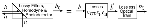
FIG. 11.: The output light $b$ is sent through a lossy output optical train, including a beam splitter, circulator, cavity filters I and II, a mixer with local oscillator light and a photodiode. The result (aside from an unimportant phase shift $\alpha_{\rm m}$) is the desired measured quantity $b_{\rm\zeta(\Omega)}$. This actual process, sketched on the left side of the equality sign, is mathematically equivalent to the idealized process sketched on the right side: The cavities’ loss effects are introduced first, producing $\breve{b}$, which is then sent through an idealized, lossless optical train including the filters.

Because the filter cavities have frequency offsets $\xi_{J}$ that make their losses different in the upper and lower side bands, the influence of the losses is most simply expressed in terms of the annihilation operators for the side bands $\breve{b}_{\pm}$, rather than in terms of the quadrature amplitudes $\breve{b}_{j}$. In terms of $b_{\pm}$, the equation describing the influence of losses is identical to that in the case of the arm cavities with fixed mirrors, Eqs. (137) with ${\cal K}=0$:

$$\breve{b}_{\pm}=\left(1-{1\over 2}\sum_{J}{\cal E}_{J\pm}\right)b_{\pm}+\sum_{J}\sqrt{{\cal E}_{J\pm}}\,n_{J\pm}\;,$$ (138)

Here (i) the sum is over the two filter cavities $J={\rm I}$ and II (which must be treated specially) and over the rest of the output optical train, denoted $J={\rm OT}$; (ii) ${\cal E}_{J}$ is the net fractional loss of photons in element $J$; (iii) $n_{J\pm}$ is the annihilation operator for the loss-noise field introduced by element $J$; (iv) for each filter I or II, the analog of the phase factor $2\beta$ of Eq. (137) gets put onto the light in the subsequent lossless filter and thus is absent here; and (v) we have absorbed a phase factor into the definition of $n_{J\pm}$.

The net fractional photon loss in a filter cavity must be identical to that in an arm cavity, Eq. (134), if written in terms of the cavity’s half bandwidth ($\gamma$ for arm cavity, $\delta_{J}$ for filter cavity) and the difference between the field’s frequency $\omega=\omega_{o}\pm\Omega$ and the cavity’s resonant frequency $\omega_{\rm res}$ ($\omega-\omega_{\rm res}=\pm\Omega$ for arm cavity; $\omega-\omega_{\rm res}=\xi_{J}\delta_{J}\pm\Omega$ for filter cavity). Therefore, Eq. (134) implies that

$${\cal E}_{J\pm}={2\epsilon_{J}\over 1+(\xi_{J}\pm\Omega/\delta_{J})^{2}}\quad\hbox{for }J={\rm I},{\rm II}\;.$$ (139)

For the remainder of the optical train, the net fractional photon loss ${\cal E}_{\rm OT}$ is the sum of the contributions from the various elements and is independent of frequency:

$${\cal E}_{{\rm OT}\pm}={\cal E}_{\rm OT}=\epsilon_{\rm bs}+\epsilon_{\rm circ}+2\epsilon_{\rm mm}+\epsilon_{\rm lo}+\epsilon_{\rm pd}\sim 0.006\;.$$ (140)

By expressing $b_{\pm}$ and $n_{J\pm}$ in terms of $b_{j}$ and $n_{Jj}$ (for $j=1,2$) via the analog of Eq. (6), inserting these expressions into Eq. (138), then computing $\breve{b}_{j}$ via the analog of Eq. (6), we obtain

$$\breve{b}_{1}=\left(1-{1\over 2}{\cal E}_{\rm OTF}\right)b_{1}-{i\over 4}\sum_{J}({\cal E}_{J+}-{\cal E}_{J-})b_{2}$$ (142)

$$+{1\over 2}\sum_{J}\left[(\sqrt{{\cal E}_{J+}}+\sqrt{{\cal E}_{J-}})n_{J1}+i(\sqrt{{\cal E}_{J+}}-\sqrt{{\cal E}_{J-}})n_{J2}\right],$$ (143)

$$\breve{b}_{2}=\left(1-{1\over 2}{\cal E}_{\rm OTF}\right)b_{2}+{i\over 4}\sum_{J}({\cal E}_{J+}-{\cal E}_{J-})b_{1}$$ (144)

$$+{1\over 2}\sum_{J}\left[(\sqrt{{\cal E}_{J+}}+\sqrt{{\cal E}_{J-}})n_{J2}-i(\sqrt{{\cal E}_{J+}}-\sqrt{{\cal E}_{J-}})n_{J1}\right]\;.$$ (145)

Here

$${\cal E}_{\rm OTF} \equiv {1\over 2}\sum_{J}({\cal E}_{J+}+{\cal E}_{J-})$$ (146)

$$= {\cal E}_{\rm OT}+{1\over 2}({\cal E}_{{\rm I}+}+{\cal E}_{{\rm I}-}+{\cal E}_{{\rm II}+}+{\cal E}_{{\rm II}-})$$ (147)

$$\simeq {\cal E}_{\rm OT}+\epsilon\sum_{J={\rm I,II}}\;\sum_{s=+,-}{\gamma/\delta_{J}\over 1+(\xi_{J}+s\Omega/\delta_{J})^{2}}$$ (148)

is the net, $\Omega$-dependent loss factor for the entire output optical train including the filter cavities. From Eqs. (128), (140) and (148) and Fig. 10, we infer that

$${\cal E}_{\rm OTF}\sim 0.009$$ (149)

with only a weak dependence on frequency, which we shall neglect.

In Eqs. (VI D), the terms $i\times($quantity linear in ${\cal E}_{J\pm})b_{j}$ [the $b_{2}$ term in $\breve{b}_{1}$ and the $b_{1}$ term in $\breve{b}_{2}$] will contribute amounts second order in the losses ($\propto{\cal E}_{J}^{2})$ to the signal and/or noise, and thus can be neglected. We shall flag our neglect of these terms below, when they arise.

E Computation of noise spectra for variational-output and squeezed-variational interferometers

The output of a squeezed-variational interferometer or variational-output interferometer is the frequency-dependent quadrature $b_{\zeta}$ depicted in Fig. 11. This quantity, when split into signal $\propto h$ plus noise $\propto\Delta\breve{b}_{\zeta}$, takes the following form:

$$b_{\zeta}=\breve{b}_{1}\cos\zeta+\breve{b}_{2}\sin\zeta$$ (150)

$$=\sin\zeta\left[\sqrt{2{\cal K}_{*}}\left(1-{1\over 2}{\cal E}_{\rm OTF}\right){h\over h_{\rm SQL}}e^{i\beta_{*}}+{\Delta\breve{b}_{\zeta}\over\sin\zeta}\right]\;;$$ (151)

cf. Eqs. (131) and (VI D). Here we have omitted an imaginary part of the factor $1-{1\over 2}{\cal E}_{\rm OTF}$ [arising from the $b_{2}$ term in $\breve{b}_{1}$, Eq. (142)] because its modulus is second order in the losses ($\propto{\cal E}_{J}^{2}$) and therefore it contributes negligibly to the signal strength.

Equation (151) implies that the gravitational-wave noise operator is

$$h_{n}=\left(1+{1\over 2}{\cal E}_{\rm OTF}+{1\over 4}{\cal E}\right){h_{\rm SQL}\over\sqrt{2{\cal K}}}e^{-i\beta_{*}}(\Delta\breve{b}_{2}+\Delta\breve{b}_{1}\cot\zeta)\;,$$ (152)

where we have used Eq. (133) for ${\cal K}_{*}$.

For a squeezed-variational interferometer, the dark-port input field $a_{j}$ is in a squeezed state, with squeeze factor $R$ and squeeze angle $\lambda(\Omega)$ (which, after optimization, will turn out to be $\lambda=\pi/2$ as for a lossless interferometer). For a variational-output interferometer, $a_{j}$ is in its vacuum state, which corresponds to squeezing with $R=0$ so we lose no generality by assuming a squeezed input. Since all the noise fields except $a_{j}$ are in their vacuum states, the light’s full input state is

$$|{\rm in}\rangle=|0_{n}\rangle\otimes|0_{n_{\rm OT}}\rangle\otimes|0_{n_{\rm I}}\rangle\otimes|0_{n_{\rm II}}\rangle\otimes S(R,\lambda)|0_{a}\rangle\;,$$ (153)

where the notation should be obvious.

The gravitational-wave noise is proportional to

$$\langle{\rm in}|h_{n}h_{n^{\prime}}|{\rm in}\rangle=\langle 0|h_{ns}h_{ns^{\prime}}|0\rangle$$ (154)

where $|0\rangle$ is the vacuum state of all the noise fields $a$, $n$, $n_{\rm OT}$, $n_{\rm I}$, and $n_{\rm II}$; and $h_{ns}$ is the usual squeezed noise operator

$$h_{ns}=S^{{\dagger}}(R,\lambda)h_{n}S(R,\lambda)\;.$$ (155)

We bring this squeezed-noise operator into an explicit form by (i) inserting Eq. (152) into Eq. (155), then (ii) replacing the $\Delta\breve{b}_{j}$’s by expressions (VI D) [with $\Delta$ put onto all the $b$’s, i.e. with the signal removed], then (iii) replacing the $\Delta b_{j}$’s by expressions (137), and then (iv) invoking Eqs. (A12) for the action of the squeeze operators on the $a_{j}$’s. The result is

$$h_{ns}=\left(1-{1\over 4}{\cal E}\right)\times\hbox{[Eq.\ (\ref{hns''})]}$$ (156)

$$+{h_{\rm SQL}\over\sqrt{2{\cal K}}}\left\{\left(-{\cal K}e^{i\beta}\sqrt{\epsilon/2}+\sqrt{{\cal E}}\cot\zeta\right)e^{i\beta}n_{1}+\sqrt{\cal E}e^{i\beta}n_{2}\right.$$ (157)

$$+{1\over 2}\sum_{J}\left[(\sqrt{{\cal E}_{J+}}+\sqrt{{\cal E}_{J-}})\cot\zeta-i(\sqrt{{\cal E}_{J+}}-\sqrt{{\cal E}_{J-}})\right]n_{J1}$$ (158)

$$\left.+{1\over 2}\sum_{J}\left[\sqrt{{\cal E}_{J+}}+\sqrt{{\cal E}_{J-}}+i(\sqrt{{\cal E}_{J+}}-\sqrt{{\cal E}_{J-}})\cot\zeta\right]n_{J2}\right\}$$ (159)

(160)

where we have omitted terms, arising from $b_{2}$ in Eq. (142) and from $b_{1}$ in Eq. (144), which contribute amounts ${\cal O}({\cal E}_{J}^{2})$ to $S_{h}$; and we have omitted a term proportional to $\beta_{*}-\beta$ which contributes an amount ${\cal O}(\epsilon^{2})$.

By virtue of Eq. (154) and the argument preceding Eqs. (33), we can regard all of the quadrature noise operators $a_{j}$, $n_{j}$, $n_{Jj}$ in this $h_{ns}$ as random processes with unit spectral densities and vanishing cross-spectral densities. Correspondingly, the gravitational-wave noise is the sum of the squared moduli of the coefficients of the quadrature noise operators in Eq. (160):

$$S_{h} = {h_{\rm SQL}^{2}\over 2{\cal K}}\Big{[}\left(1-{1\over 2}{\cal E}\right)\left(1+{\tilde{\cal K}}^{2}\right)$$ (163)

$$\times\{e^{-2R}+\sinh 2R[1-\cos 2(\tilde{\Phi}+\lambda)]\}$$

$$+{\cal K}^{2}{\epsilon\over 2}+(1-\tilde{\cal K}\cot\zeta){\cal E}+(1+\cot^{2}\zeta){\cal E}_{\rm OTF}\Big{]}$$

where

$${\tilde{\cal K}}={\cal K}-\cot\zeta\;,\quad\tilde{\Phi}={\rm arccot\tilde{\cal K}}$$ (164)

[Eq. (87)]. In Eq. (163), the first two lines come from $a_{1}$ and $a_{2}$ [squeezed vacuum entering the dark port; cf. Eq. (89)] modified by losses in the arm cavities [the factor $1-{\cal E}/2$)]; the first two terms on the third line come from $n_{1}$ and $n_{2}$ [shot noise due to vacuum entering at loss points in the arm cavities]; and the last term comes from $n_{J1}$ and $n_{J2}$ [shot noise due to vacuum entering at loss points in the output optical train, including the filters].

As for the lossless interferometer [Eqs. (90) and (92)], the noise (163) is minimized by setting the input squeeze angle $\lambda$ and output homodyne phase $\zeta$ to

$$\lambda=\pi/2\;,\quad\zeta=\Phi\equiv{\rm arccot}{\cal K}\;$$ (165)

[aside from a neglible correction $\delta\zeta=({\cal E}+2{\cal E}_{\rm OTF})e^{-2R}/$ $({\cal K}+{\cal K}^{-1})$]. This optimization produces $\tilde{\cal K}=0$ and $\lambda=\tilde{\Phi}=\pi/2$, so

$$S_{h}={h_{\rm SQL}^{2}\over 2}$$ (166)

$$\times\left[{\left(1-{1\over 2}{\cal E}\right)e^{-2R}+{\cal E}+{\cal E}_{\rm OTF}\over{\cal K}}+{\cal K}\left({\epsilon\over 2}+{\cal E}_{\rm OTF}\right)\right]\;.$$ (167)

Note that the optimization has entailed a squeezed input with frequency-independent squeeze phase, as in the lossless interferometer; so no filters are needed in the input. The output filters must produce a FD homodyne angle $\zeta=\Phi(\Omega)$ that is the same as in the lossless case and therefore can be achieved by two long, Fabry-Perot cavities.

It is instructive to compare the noise (166) for a lossy squeezed-variational interferometer with that (92) for one without optical losses. In the absence of losses, the output’s FD homodyne detection can completely remove the radiation-pressure back-action noise from the signal; only the shot noise, $\propto 1/{\cal K}\propto 1/I_{o}$, remains. Losses in the interferometer’s arm mirrors prevent this back-action removal from being perfect: they enable a bit of vacuum field $n$ to leak into the arm cavities, and this field produces radiation-pressure noise that remains in the output after the FD homodyne detection (the ${\cal K}\epsilon/2$ term in Eq. (166)].

The ${\cal K}{\cal E}_{\rm OTF}$ noise in Eq. (166) has the same dependence on laser power, $\propto{\cal K}\propto I_{o}$, as the radiation-pressure noise. Nevertheless, it is actually shot noise, not radiation pressure noise. It is produced by the vacuum loss-noise fields that leak into the output signal light when it encounters each lossy optical element. Those fields’ shot noise gets weighted by the factor $\cot\zeta=\cot\Phi={\cal K}$ in the homodyne process, which accounts for their proportionality to ${\cal K}\propto I_{o}$.

A reasonable estimate for the amount of input-light squeezing that might be achieved in LIGO-III is[33]

$$e^{-2R}\simeq 0.1\;.$$ (168)

By contrast, Eqs. (128), (130), (134) and (148) suggest

$$({\cal E}+{\cal E}_{\rm OTF})\sim 0.01\;.$$ (169)

This motivates our neglecting ${\cal E}+{\cal E}_{\rm OTF}$ compared to $e^{-2R}$ in expression (166), and rewriting the noise (166) as

$$S_{h}\simeq{h_{\rm SQL}^{2}\over 2}\left[{e^{-2R}\over{\cal K}}+{\cal K}\epsilon_{*}\right]\;,$$ (170)

where

$$\epsilon_{*}\equiv{\epsilon\over 2}+{\cal E}_{\rm OTF}\sim 0.0010\;;$$ (171)

cf. Eqs. (128) and (149).

Equation (170) is our final form for the noise spectrum of a lossy squeezed-variational interferometer. When we set the input squeeze factor to unity, $e^{-2R}=1$, it becomes the noise spectrum for a lossy variational-output interferometer:

$$S_{h}\simeq{h_{\rm SQL}^{2}\over 2}\left[{1\over{\cal K}}+{\cal K}\epsilon_{*}\right]\;,$$ (172)

Errors $\Delta\lambda=\lambda-\pi/2$ in the input squeeze angle and $\Delta\zeta=\zeta-{\rm arccot}{\cal K}$ in the output homodyne phase will increase the noise spectral density. By performing a power series expansion of expression (163), we obtain for the noise increase

$$\Delta S_{h} = {h_{\rm SQL}^{2}\over{\cal K}}\left[\sinh 2R\;\Delta\lambda^{2}-2(1+{\cal K}^{2})\sinh 2R\;\Delta\lambda\Delta\zeta\right.$$ (174)

$$\quad\quad\quad\left.+{(1+{\cal K})^{2}e^{2R}\over 2}\;\Delta\zeta^{2}\right]$$

$$\simeq {h^{2}_{\rm SQL}\over 2{\cal K}}e^{2R}[\Delta\lambda-(1+{\cal K}^{2})\Delta\zeta]^{2}\;,$$ (175)

where the second expression is accurate in the limit $e^{2R}\gg e^{-2R}$. Numerical evaluations show that, for $e^{-2R}=0.1$ and $\epsilon_{*}=0.01$ (see above), and for ${\cal K}\sim 1$ to $3$ (the range of greatest interest; cf. Sec. VII), $\Delta\sqrt{S_{h}}$ will be less than ${1\over 4}\sqrt{S_{h}}$ so long as: (i) the input squeeze angle is accurate to $|\Delta\lambda|\lesssim 0.05$, and (ii) the FD output homodyne phase is accurate to $|\Delta\zeta|\lesssim 0.01$. At ${\cal K}=1$ the FD phase’s required accuracy is reduced to $|\Delta\zeta|\lesssim 0.04$. The FD phase $\zeta$ is determined by the filter cavities’ half bandwidths $\delta_{J}$ and fractional frequency offsets $\xi_{J}$, and the local oscillator phase or equivalently the final, conventional homodyne detector’s homodyne phase $\theta$. The filter cavities’ half bandwidths $\delta_{J}$ (or equivalently their finesses) are fixed by the mirror coatings. Coating-produced errors in $\delta_{J}$ can be compensated to some degree by tuning the fractional frequency offsets $\xi_{J}$ (via adjusting the mirror positions) and by tuning the local oscillator phase or equivalently $\theta$. Finesse errors as large as five per cent, $|\Delta\delta_{J}|/\delta_{J}\lesssim 0.05$, can be compensated to yield the required $|\Delta\zeta|\lesssim 0.01$ by tuning the offsets and homodyne phase to one percent accuracy, $|\Delta\xi_{J}|\lesssim 0.01$, $\Delta\theta\lesssim 0.01$ [Eqs. (105), (C2), (C3) and Fig. 10]. These requirements are challenging.

F Computation of the noise spectrum for a squeezed-input interferometer

For a squeezed-input interferometer, as for squeezed-variational, the losses in the input optical train influence the noise only through their impact on the squeeze factor $e^{-2R}\sim 0.1$ of the dark-port vacuum when it enters the arm cavities. By contrast, losses in the arm cavities and in the output optical train will produce noise in much the same manner as they do for a squeezed-variational interferometer. More specifically:

The effect of arm-cavity and output-train losses on the squeezed noise operator $h_{ns}$ can be read off of the squeezed-variational formula (160) as follows: (i) Set $\zeta=\pi/2$ so the quantity measured is $\breve{b}_{2}$ [no output filtering; Eq. (151)]; (ii) correspondingly set $\cot\zeta=0$, $\tilde{\cal K}={\cal K}$, and $\tilde{\Phi}=\Phi\equiv{\rm arccot}{\cal K}$ [Eqs. (164)]; (iii) in the sum over $J$ include only $J={\rm OT}$ and not $J={\rm I,II}$ since there are no output filters. The result is

$$h_{ns}=\left(1-{1\over 4}{\cal E}\right)\times\hbox{[Eq.\ (\ref{hnsExpand})]}$$ (176)

$$+{h_{\rm SQL}\over\sqrt{2{\cal K}}}\left(-{\cal K}\sqrt{\epsilon/2}\;e^{2i\beta}n_{1}+\sqrt{\cal E}e^{i\beta}n_{2}+\sqrt{{\cal E}_{\rm OT^{\prime}}}\;n_{\rm OT^{\prime}2}\right)\;.$$ (177)

(178)

Here the prime on the subscript OT indicates that we must omit losses due to mode-matching into the output filters and mixing with the local oscillator, since there are no output filters or homodyne detection. Correspondingly,

$${\cal E}_{\rm OT^{\prime}}=\epsilon_{\rm bs}+\epsilon_{\rm circ}+\epsilon_{\rm pd}\sim 0.003$$ (179)

is the net fractional photon loss in the output optical train.

Treating the quadrature noise operators as random processes with unit spectral density and vanishing cross spectral densities, we read off $S_{h}$ from Eq. (178):

$$S_{h}={h^{2}_{\rm SQL}\over 2}\Bigg{[} {{\cal E}+{\cal E}_{\rm OT^{\prime}}\over{\cal K}}+{\epsilon\over 2}{\cal K}+\left(1-{1\over 2}{\cal E}\right)\left({1\over{\cal K}}+{\cal K}\right)$$ (181)

$$\times\{\cosh 2R-\cos[2(\lambda+\Phi)]\sinh 2R\}\Bigg{]}\;.$$

As in the lossles case, the noise is minimized by squeezing the dark-port input at the FD angle $\lambda(\Omega)=-\Phi\equiv-{\rm arccot}{\cal K}$ [Eq. (60)]. The result is

$$S_{h}={h^{2}_{\rm SQL}\over 2} \left[\left(1-{1\over 2}{\cal E}\right)\left({1\over{\cal K}}+{\cal K}\right)e^{-2R}\right.$$ (183)

$$\left.+{{\cal E}+{\cal E}_{\rm OT}\over{\cal K}}+{\epsilon\over 2}{\cal K}\right]\;.$$

For our estimated squeezing $e^{-2R}\sim 0.1$ and losses ${\cal E}_{\rm OT^{\prime}}\sim{\cal E}\sim\epsilon\lesssim 0.003$ in the LIGO-III time frame, the loss parameters are small compared to the squeeze, and thus contribute negligibly to the noise, so $S_{h}$ is well approximated by the lossless formula

$$S_{h}\simeq{h_{\rm SQL}^{2}\over 2}\left({1\over{\cal K}}+{\cal K}\right)e^{-2R}\;.$$ (184)

However, it is important to keep in mind that the input squeeze factor $e^{-2R}$ is constrained not only by the physics of the squeezing appratus, but also by losses in the input optical train and mode matching into the arm cavities.

By expanding expression (181) in powers of $\Delta\lambda=\lambda+{\rm arccot}{\cal K}$, we see that the fractional increase in noise due to errors in the FD squeeze angle is

$${\Delta\sqrt{S_{h}}\over\sqrt{S_{h}}}=e^{2R}\sinh 2R\;\delta\lambda^{2}\simeq{e^{4R}\over 2}\Delta\lambda^{2}\;.$$ (185)

For $e^{-2R}=0.1$, this fractional noise increase will be less than 1/4 so long as $\Delta\lambda$ is less than $0.07$. This translates into accuracies of $\sim 7$ per cent for the prefilter squeeze angle, $\sim 15$ per cent for the filter cavities’ fractional frequency offsets ($|\Delta\xi_{J}|\lesssim 0.15$), and $\sim 10$ per cent for the cavities’ half bandwidths or equivalently their finesses ($\Delta\delta_{J}/\delta_{J}\lesssim 0.1$). These constraints are significantly less severe than those for a squeezed-variational interferometer (end of Sec. VI E); but, as we shall see, the potential performance of this squeezed-input interferometer is poorer by a factor $\sim 1.5$ – 2 than that of the squeezed-variational one.

VII Discussion of the Interferometers’ Noise Spectra

The noise spectra for our three lossy QND interferometers, Eqs. (170), (172) and (184), all have the same universal form—a form identical to that for a conventional broadband interferometer, Eq. (34). Only the parameters $\mu$ and $\sigma$ characterizing the noise differ from one interferometer to another. This universal form can be written as

$${\sqrt{S_{h}(\Omega)}\over h_{\rm SQL}(\Omega)}=\mu\sqrt{{1\over 2}\left({\Omega_{*}^{2}\over\sigma^{2}}+{\sigma^{2}\over\Omega_{*}^{2}}\right)}\;,$$ (187)

where $\Omega_{*}$ is the following function of angular frequency

$$\Omega_{*}\equiv{\Omega\over\gamma}\sqrt{{1+\Omega^{2}/\gamma^{2}}\over 2}$$ (188)

and $h_{\rm SQL}(\Omega)$ is given by Eq. (27). Notice that $\Omega_{*}=1$ when $\Omega=\gamma\simeq 100$ Hz; $\Omega_{*}=(\Omega/\gamma)/\sqrt{2}$ when $\Omega\ll\gamma$, and $\Omega_{*}=(\Omega/\gamma)^{2}/\sqrt{2}$ when $\Omega\gg\gamma$.

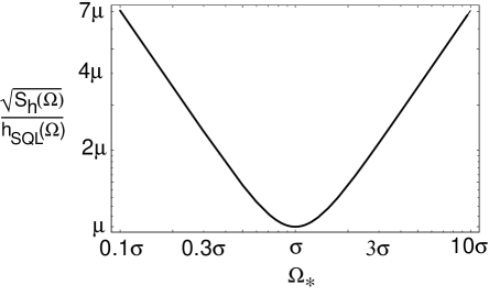
FIG. 12.: Universal noise curve for conventional and QND interferometers [Eqs. (188)].

This universal noise curve is plotted as a function of $\Omega_{*}$ in Fig. 12. Its two parameters are the minimum value $\mu$ of the noise, i.e. the minimum amplitude noise in units of the SQL, and the dimensionless frequency $\sigma$ (in units of $\Omega_{*}$) at which the noise takes on this minimum value.

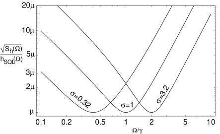
FIG. 13.: Universal noise curve plotted as a function of angular frequency $\Omega$ for various values of the dimensionless frequency parameter $\sigma$.

Figure 13 shows this universal noise curve plotted as a function of angular frequency $\Omega$. Notice that, because of the relation (188) between $\Omega_{*}$ and $\Omega$, the shape of the noise curve depends modestly on the location $\sigma$ of its minimum.

The values of the parameters $\mu$ and $\sigma$ for our various interferometer configurations are shown in Table II. Notice the following details of this table: (i) The minimum noise $\mu$ (the optimal amount by which the SQL can be beat) is independent of the laser input power $I_{o}$ in all cases; it depends only on the level of input squeezing $e^{-2R}$ and the level of losses $\epsilon_{*}$. (ii) For our estimated loss level and squeeze level, the squeezed-input interferometer and variational-output interferometer achieve the same $\mu\simeq 0.32$, while the squeezed-variational interferometer achieves a moderately lower $\mu\simeq 0.18$. (iii) The frequency $\Omega_{*}=\sigma$ at which the minimum noise is achieved is proportional to $\sqrt{I_{o}/I_{\rm SQL}}$. (Recall that $I_{\rm SQL}$ is the input power required for a conventional interferometer to reach the SQL at the angular frequency $\Omega=\gamma\simeq 2\pi\times 100$ Hz, i.e. at $\Omega_{*}=1$; to do so, the conventional interferometer must have $\sigma=1$.) (iv) For $I_{o}=I_{\rm SQL}$, the squeezed-input interferometer has $\sigma=1$, but the variational-output and squeezed-variational interferometers have $\sigma<1$, which means that the minimum of the noise curve is at $\Omega<\gamma\simeq 100$ Hz. To push $\sigma$ up to unity, i.e. to push the noise-curve minimum up to $\Omega=\gamma$, requires $I_{o}/I_{\rm SQL}=1/\sqrt{\epsilon_{*}}\simeq 10$ in a variational-output interferometer, and $I_{o}/I_{\rm SQL}=\sqrt{e^{-2R}/\epsilon_{*}}\simeq 3.2$ in a squeezed-variational interferometer.

TABLE II.: The values of the parameters $\mu=($minimum noise) and $\sigma=($frequency of minimum) for various interferometer (“IFO”) configurations: Conv = Conventional broadband [Eq. (34)], SI = Squeezed-Input [Eq. (184)], VO = Variational-Output [Eq. (172)], and SV = Squeezed-Variational [Eq. (170)]. The numerical values are for $e^{-2R}=0.1$ and $\epsilon_{*}=0.01$.

IFO	$\mu$	$\sigma$
Conv.	1	$\sqrt{I_{o}/I_{\rm SQL}}$
SI	$\sqrt{e^{-2R}}\simeq 0.32$	$\sqrt{I_{o}/I_{\rm SQL}}$
VO	$\epsilon_{*}^{1/4}\simeq 0.32$	$\sqrt{I_{o}/I_{\rm SQL}\over 1/\sqrt{\epsilon_{*}}}\simeq\sqrt{I_{o}/I_{\rm SQL}\over 10}$
SV	$(e^{-2R}\epsilon_{*})^{1/4}\simeq 0.18$	$\sqrt{I_{o}/I_{\rm SQL}\over\sqrt{e^{-2R}/\epsilon_{*}}}\simeq\sqrt{I_{o}/I_{\rm SQL}\over 3.2}$

The importance of pushing $\sigma$ up to unity or higher is explained in Fig. 14. This figure requires some discussion:

The most promising gravitational waves for LIGO are those from the last few minutes of inspiral of black-hole/black-hole binaries, black-hole/neutron-star binaries, and neutron-star/neutron-star binaries. The amplitude signal-to-noise ratio $S/N$ produced by these waves is given by

$${S^{2}\over N^{2}}=4\int_{0}^{\infty}{|\tilde{h}|^{2}\over S_{h}}{d\Omega\over 2\pi}=4\int_{-\infty}^{\infty}{|\Omega\tilde{h}|^{2}\over\Omega S_{h}}{d\ln\Omega\over 2\pi}\;,$$ (189)

where $\tilde{h}$ is the Fourier transform of the waveform $h(t)$. For the inspiraling binary $|\Omega\tilde{h}|$ is nearly independent of frequency throughout the LIGO band [34], so the signal-to-noise ratio is optimized by making $\Omega S_{h}(\Omega)$ as small as possible over as wide a range of $\ln\Omega$ as possible.

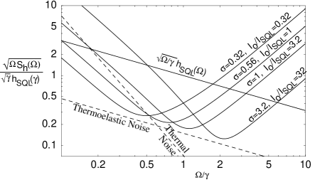
FIG. 14.: Noise curves for SQL interferometers with noise minima $\mu=0.18$ and various values of the frequency parameter $\sigma$. The vertical axis is weighted by $\sqrt{\Omega/\gamma}$ so the curves give an indication of the relative noise in searches for waves from inspiraling binaries; see text. The noise curves are labeled by the power $I_{o}/I_{\rm SQL}$ required by a squeezed-variational interferometer to achieve the given $\sigma$.

Figure 14 plots $\sqrt{\Omega S_{h}(\Omega)}$ as a function of $\Omega/\gamma$ using logarithmic scales on both axes, and using the minimum-noise parameter $\mu=0.18$ corresponding to our fiducial squeezed-variational interferometer (though the specific value of $\mu$ is irrelevant to our present discussion). From the shapes of the curves it should be evident that the larger is the frequency of the noise minimum, i.e. the larger is $\sigma$ at fixed $\mu$, the larger will be the $S/N$ for inspiraling binaries.

A second factor dictates using large $\sigma$, in particular $\sigma\gtrsim 1$. This is thermal noise in the interferometer’s test-mass suspension fibers. The thermal noise scales with frequency as $\sqrt{\Omega S_{h}^{\rm thermal}(\Omega)}\propto\Omega^{-2}$ or $\propto\Omega^{-5/2}$ depending on the nature of the dissipation [35]; see the steep dashed curve in Fig. 14. It seems realistic to expect, in LIGO-III, that this thermal noise will be at approximately the level shown in the figure, so it compromises the performance of QND interferometers at $\Omega\lesssim 0.5\gamma\simeq 50$ Hz [7, 36]. Correspondingly, to avoid the thermal noise significantly debilitating the $S/N$ for inspiraling binaries, it will be necessary to have $\sigma\gtrsim 1$.

Because $\sigma$ scales as $\sqrt{I_{o}/I_{\rm SQL}}$ for all interferometer designs, large $\sigma$ entails large laser power. In particular, $\sigma\gtrsim 1$ requires $I_{o}\gtrsim I_{\rm SQL}$; cf. Table II. For our fiducial parameters (Table I), $I_{\rm SQL}=10$ kW, which corresponds to an optical power circulating in each of the interferometer’s arm cavities

$$W_{\rm circ}^{\rm SQL}={I_{\rm SQL}/2\over\gamma L/c}={mcL\gamma^{3}\over 8\omega_{o}}=0.62\;\hbox{MW}\;.$$ (190)

To construct mirrors capable of handling this huge power will be an enormous technical challenge (even though this is approximately the circulating power contemplated for LIGO-II). To operate with a circulating power much larger than this might not be possible. Therefore, it may be important in LIGO-III to achieve $\sigma\gtrsim 1$ while keeping $I_{o}/I_{\rm SQL}$ not much larger than unity.

The squeezed-input interferometer, with its $\sigma=\sqrt{I_{o}/I_{\rm SQL}}$ (Table II) is the most attractive from this point of view [and also in terms of its required filter and squeeze-phase accuracies; cf. end of Sec. VI F]; and the variational-output with its $\sigma=\sqrt{\sqrt{\epsilon_{*}}I_{o}/I_{\rm SQL}}\simeq\sqrt{0.1I_{o}/I_{\rm SQL}}$ is the least attractive. The squeezed-variational interferometer, with $\sigma=\sqrt{\sqrt{\epsilon_{*}/e^{-2R}}I_{o}/I_{\rm SQL}}\simeq\sqrt{0.32I_{o}/I_{\rm SQL}}$ requires a modestly higher laser power to reach $\sigma=1$ than the squeezed-input [and requires better filter and squeeze-phase accuracies], but it is capable of a lower noise minimum, $\mu\simeq(e^{-2R}\epsilon_{*})^{1/4}\simeq 0.18$ vs. $\mu=\sqrt{e^{-2R}}\simeq 0.32$ for squeezed-input.

This suggests an R&D strategy: Focus on input squeezing as a key foundation for LIGO-III (it is needed both for squeezed-input and squeezed-variational interferometers), and in parallel (i) develop the technology and techniques for the FD homodyne detection required by squeezed-variational configurations, (ii) work to drive down optical losses to the levels $\epsilon\sim\epsilon_{\rm circ}\sim\epsilon_{\rm bs}\sim\epsilon_{\rm mm}\sim\epsilon_{\rm lo}\sim\epsilon_{\rm pd}\sim 0.001$ [Eq. (126)], and (since ponderomotive squeezing, which underlies all our QND interferometers, has never been seen) (iii) carry out experiments in a small test appratus to demonstrate ponderomotive squeezing and to search for unexpected obstacles and imperfections in it.

If both input squeezing and FD homodyne detection can be implemented successfully, then the squeezed-variational interferometer is likely to achieve better performance than any other configuration discussed in this paper, despite its apparent need for higher laser power (e.g. $I_{o}/I_{\rm SQL}\simeq 3.2$ to achieve $\sigma=1$ compared to $I_{o}/I_{\rm SQL}=1$ for squeezed input, with our fiducial parameters). If powers as high as $I_{o}/I_{\rm SQL}\simeq 3.2$ cannot be handled, then we can operate the squeezed-variational interferometer with a lower power without much loss of performance.

Consider, for example, $\sqrt{S_{h}}/h_{\rm SQL}$ evaluated at $\Omega=\sigma\simeq 2\pi\times 100$ Hz, as a function of $I_{o}/I_{\rm SQL}$ in a variational-output interferometer with our fiducial $e^{-2R}=0.1$ and $\epsilon_{*}=0.01$. The optimal $I_{o}/I_{\rm SQL}=3.2$ produces $\sqrt{S_{h}(\gamma)}/h_{\rm SQL}=0.18$; pushing $I_{o}/I_{\rm SQL}$ down by a factor 2, to 1.6, increases the noise at $\Omega=\gamma$ by only 10 percent, to 0.20; pushing down all the way to $I_{o}/I_{\rm SQL}=1$ increases the noise to only $\sqrt{S_{h}(\gamma)}/h_{\rm SQL}=0.23$, which is still significantly lower noise than the optimized squeezed-input interferometer ($0.32$ at $I_{o}/I_{\rm SQL}=1$).

It is worth recalling that for noncosmological sources (sources at distance $\ll 3$ Gpc), the volume of the universe that can be searched for a given type of source scales as the inverse cube of the amplitude noise, so a noise level $\sqrt{S_{h}}/h_{\rm SQL}=0.18$ corresponds to search-volume increase of $1/0.18^{3}\simeq 180$ over a SQL-limited interferometer, i.e. over LIGO-II.

VIII Conclusions

In this paper we have explored three candidate ideas for QND LIGO-III interferometers: squeezed-input, variational-output, and squeezed variational. The squeezed-input and squeezed-variational interferometers both looks quite promising. For our estimated levels of optical loss and levels of squeezing, and for an input laser power $I_{o}/I_{\rm SQL}=1$ (the LIGO-II level), the squeezed-input interferometer could achieve a noise $\mu\simeq 0.32$ of the SQL, with a corresponding increase ${\cal V}\simeq 1/0.32^{3}\simeq 30$ over LIGO-II in the volume of the universe that could be searched for a given source, at non-cosmological distances. The squeezed-variational interferometer could achieve $\mu\simeq 0.23$ of the SQL with a search-volume increase over LIGO-II of ${\cal V}\simeq 80$. If the optics can handle a laser power $I_{o}/I_{\rm SQL}\simeq 3.2$, then the squeezed-variational interferometer could reach $\mu\simeq 0.18$ of the SQL and a search-volume increase of ${\cal V}\simeq 180$. These numbers scale with the losses, squeezing, and laser power as shown in Table II.

The squeezed-input and squeezed-variational designs are therefore sufficiently promising to merit serious further study. Some of the issues that need theoretical analysis are:

• How can one incorporate into these interferometer designs the various light modulations that are required, in a real gravitational-wave interferometer, to (i) make the interferometer be shot-noise limited (put the gravitational-wave signal into $\sim 100$ Hz sidebands of a MHz modulation), (ii) control the mirror positions and orientations, … [37].

• What accuracies and other characteristics are needed for the interferometers’ new elements: the circulator, filter cavities, and input squeezing? How can these be achieved? For example, how stable must be the local oscillator for the conventional homodyne detector, and can it be achieved simply by tapping some light off the interferometer’s output or input beam?

• If the filter cavities are placed in the same long vacuum tubes as the interferometer’s arm cavities (with their enormous circulating power), what will be the nature and level of noise due to scattering of light from the test-mass cavites to the filter cavities? (We thank Eanna Flanagan for raising this issue.)

• Can the filter cavities be made to serve multiple purposes? For example, is it possible to use a single optical cavity for both filters, e.g., with the two filters based on two different polarization states (for which the filter might be made to behave differently via birefringence), or with the two filters based on different, adjacent longitudinal modes? As another example, could an output filter cavity be used as a source of ponderomotively squeezed vacuum for input into the interferometer’s dark port?

• Signal recycling via resonant-sideband extraction (RSE) [38] is likely to be a standard tool in LIGO-II [7]. How can one best implement RSE simultaneously with the FD homodyne detection (and input squeezing) of a variational-output (or squeezed-variational) interferometer? [37] How can one best achieve the FD homodyne’s filtration [which will entail a different frequency dependence $\Phi(\Omega)$ from that in this paper’s non-RSE designs]?

• In this paper’s analysis we have made a number of simplifying approximations [e.g., our approximating the phase of the coefficient of $f_{j}$ in Eq. (B31) by $2\beta$ an approximation that fails by a frequency-dependent amount which can be nearly as large as one per cent]. At what level of sensitivity do these approximations become problematic (e.g., for our proposed two-cavity way of achieving the necessary FD homodyne detection), and how can the resulting problems be overcome?

• Our analysis is based on the crucial assumption that the interferometer’s output is strictly linear in its input [4]. Matsko and Vyatchanin [39] have shown that this is not quite correct. In the interferometer’s arms the back-action-induced mirror displacement $X$ produces a phase shift of reflected light given by $e^{-2i\Omega X/c}$, which our linearized analysis approximates as $1-2i\Omega X/c$ [cf. Eq. (B16)]; when the better approximation $1-2i\Omega X/c-2(\Omega X/c)^{2}$ is used, the result is additional, nonlinear noise, which limits the cancellation of the back-action noise by the shot noise and produces a limit [39]

  $$S_{h}^{\rm NL}\sim{h^{2}_{\rm SQL}\over{2\;{\cal N}_{\rm SQL}^{1/5}}}\sim 5\times 10^{-5}h_{\rm SQL}^{2}$$ (191)

  on the sensitivity that any of our QND designs can achieve. Here

  $${\cal N}_{\rm SQL}={I_{\rm SQL}\over\hbar\omega_{o}\gamma}={1\over 2}\left({Tc/4\omega_{o}\over\sqrt{\hbar/m\gamma}}\right)^{2}\simeq 2\times 10^{20}$$ (192)

  is the number of quanta entering a SQL interferometer in time $\gamma^{-1}\sim 2$ ms. The nonlinear limitation (191) is sufficiently far below the SQL that we need not be concerned about it. Are there any other, more serious sources of nonlinearity that might compromise the performance of these interferometers?

Experimental studies are also needed as foundations for any possible implementation of variational-output or squeezed-variational interferometers [40]. Examples are

• Studies of the debilitating effects of very high circulating powers, $W_{\circ}\sim$ a few MW, and how to control them.

• A continuation of efforts to achieve large squeezing, robustly, via nonlinear optics [33], and exploration of the possibility to do so ponderomotively [41, 42, 43, 44].${}^{\ref{foot:PondVacuum}}$

• A continuation of efforts to achieve low levels of losses in optical cavities and interferometers, so as to minimize the contamination of squeezed light by ordinary vacuum[45].

• Prototyping of FD homodyne detection by the technique proposed in this paper: filtration followed by conventional homodyne detection.

In the meantime, and in parallel with such studies, it is important to push hard on the effort to find practical QND designs that entail circulating light powers well below 1 MW [13], and that might be much less constrained by optical losses than the designs explored in this paper.

A Rotation and Squeeze Operators

In this paper we make extensive use of squeeze operators and some use of rotation operators. In this appendix we list properties of these operators that are be useful in verifying statements made the text. This appendix is based on the formalism for 2-photon quantum optics developed by Caves and Schumaker [26, 27].

The rotation operator $R(\theta)$, which acts on the Hilbert space of the modes with frequencies $\omega=\omega_{o}\pm\Omega$, is defined by

$$R(\theta)=\exp[-i\theta(a_{+}^{{\dagger}}a_{+}+a_{-}^{{\dagger}}a_{-})]$$ (A1)

(Eq. (4.33) of [26]); here $a_{\pm}$ are the annihilation operators, and $a_{\pm}^{{\dagger}}$ the creation operators for photons in these modes. This operator is unitary and has the inverse

$$R^{-1}(\theta)=R^{{\dagger}}(\theta)=R(-\theta)\;.$$ (A2)

The effect of a rotation on the modes’ annihilation operators is

$$R(\theta)a_{\pm}R^{{\dagger}}(\theta)=a_{\pm}e^{i\theta}\;$$ (A3)

(Eq. (4.35) of [26]), and its effect on the two-photon quadrature amplitudes [Eqs. (6)] is

$$R(\theta)a_{1}R^{{\dagger}}(\theta) = a_{1}\cos\theta-a_{2}\sin\theta\;,$$ (A4)

$$R(\theta)a_{2}R^{{\dagger}}(\theta) = a_{1}\sin\theta+a_{2}\cos\theta\;$$ (A5)

(Eq. (4.36) of [26]).

The squeeze operator also acts on the Hilbert space of modes with frequencies $\omega=\omega_{o}\pm\Omega$, and is defined by

$$S(r,\phi)=\exp[r(a_{+}a_{-}e^{-2i\phi}-a_{+}^{{\dagger}}a_{-}^{{\dagger}}e^{2i\phi})]$$ (A6)

(Eq. (4.9) of [26]; Eq. (1.8) of [27]). This squeeze operator is unitary and its inverse is

$$S^{-1}(r,\phi)=S^{{\dagger}}(r,\phi)=S(-r,\phi)=S(r,\phi+\pi/2)$$ (A7)

(Eq. (1.9) of [27]). The effect of a squeeze on the modes’ annihilation operators is

$$S(r,\phi)a_{\pm}S^{{\dagger}}(r,\phi)=a_{\pm}\cosh r+a_{\mp}^{{\dagger}}e^{2i\phi}\sinh r$$ (A8)

(Eq. (4.10) of [26]). From this equation and the definition (6) of the quadrature amplitudes, we infer the effect of a squeeze on those amplitudes

$$S(r,\phi)a_{1}S^{{\dagger}}(r,\phi) = a_{1}(\cosh r+\sinh r\cos 2\phi)$$ (A10)

$$+a_{2}\sinh r\sin 2\phi\;,$$

$$S(r,\phi)a_{2}S^{{\dagger}}(r,\phi) = a_{2}(\cosh r-\sinh r\cos 2\phi)$$ (A12)

$$+a_{1}\sinh r\sin 2\phi\;.$$

B Input-Output Relations for Interferometers

In this appendix we shall derive the input-output relations for the fields $a_{j}$ and $b_{j}$ that enter and leave the interferometer’s dark port. From the outset we shall include optical losses in our derivation, thereby obtaining the lossy input-output relations (131) and (137); the lossless input-output relations (23) then follow by setting $\epsilon=0$.

1 Fields at beam splitter

We describe the field amplitudes entering and leaving the beam splitter by the notation shown in Fig. 15 (cf. Fig. 3. We idealize the beam splitter as lossless in this appendix, and deal with its losses in the body of the paper in the manner sketched in Fig. 11. The amplitudes $D\;\&\;d$ of the field entering the beam splitter from the laser are defined by the following formulae for the positive-frequency part of the electric field

$$E^{(+)}_{\rm in}=\sqrt{2\pi\hbar\omega_{o}\over{\cal A}c}$$ (B1)

$$\quad\times e^{-i\omega_{o}t}\left[D+\int_{0}^{\infty}\left(d_{+}e^{-i\Omega t}+d_{-}e^{+i\Omega t}\right){d\Omega\over 2\pi}\right]\;.$$ (B2)

[cf. Eq. (5)] and for the total electric field

$$E_{\rm in}=\sqrt{4\pi\hbar\omega_{o}\over{\cal A}c}$$ (B3)

$$\quad\times\left\{\cos(\omega_{o}t)\left[\sqrt{2}D+\int_{0}^{\infty}\left(d_{1}e^{-\i\Omega t}+d_{1}^{{\dagger}}e^{+i\Omega t}\right){d\Omega\over 2\pi}\right]\right.$$ (B4)

$$\quad\quad+\left.\sin(\omega_{o}t)\int_{0}^{\infty}\left(d_{2}e^{-\i\Omega t}+d_{2}^{{\dagger}}e^{+i\Omega t}\right){d\Omega\over 2\pi}\right\}\;.$$ (B5)

Thus, $D$ is the classical amplitude of the laser light (carrier with frequency $\omega_{o}$), $d_{\pm}$ are the annihilation operators for the $\omega_{o}\pm\Omega$ sidebands, and $d_{1}$ and $d_{2}$ are the quadrature amplitudes for the side bands. [Notice that the factor out front is a $\sqrt{2\pi}$ in Eq. (B2) but $\sqrt{4\pi}$ in (B5), and notice the $\sqrt{2}D$ in (B5).] The light power $I_{o}$ impinging on the beam splitter is related to the classical amplitude $D$ by

$$I_{o}={\overline{E_{\rm in}^{2}}\over 4\pi}{\cal A}c=\hbar\omega_{o}D^{2}\;,$$ (B6)

where the overbar means time average. (Note that $D^{2}$ has dimensions Hz = 1/sec.)

For all other fields the classical amplitude and sideband amplitudes are as indicated in the figure; for example, the field going toward the east cavity has classical amplitude $D/\sqrt{2}$ and quadrature amplitudes $f^{e}_{1}$, $f^{e}_{2}$.

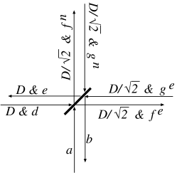
FIG. 15.: Field amplitudes entering and leaving the beam splitter (which here is idealized as lossless). The various amplitudes are defined in Eqs. (B2)–(B8).

With an appropriate choice of conventions [46], the fields’ junction conditions at the splitter are

$$f_{j}^{n}={d_{j}+a_{j}\over\sqrt{2}}\;,\quad f_{j}^{e}={d_{j}-a_{j}\over\sqrt{2}}\;,$$ (B7)

$$b_{j}={g_{j}^{n}-g_{j}^{e}\over\sqrt{2}}\;,\quad e_{j}={g_{j}^{n}+g_{j}^{e}\over\sqrt{2}}\;.$$ (B8)

Here $j=1$ or $2$.

2 Arm cavities and fields

The east and north arm cavities are presumed to be identical, with power reflection and transmission coefficients $R$ and $T$ for the front mirror, and $\tilde{R}$ and $\tilde{T}$ for the back mirror. The amplitude reflection and transmission coefficients are chosen be real, with signs $\{+\sqrt{T},-\sqrt{R}\}$, $\{+\sqrt{\tilde{T}},-\sqrt{\tilde{R}}\}$ for light that impinges on a mirror from outside the cavity; and $\{+\sqrt{T},+\sqrt{R}\}$, $\{+\sqrt{\tilde{T}},+\sqrt{\tilde{R}}\}$ for light that impinges from inside the cavity.

The dominant optical losses are for light impinging on mirrors from inside the cavity (cf. Sec. VI B). The influence of the losses on the interferometer’s signal and noise are independent of the physical nature of the losses—whether it is light scattering off a mirror, absorption in the mirror, or transmission through the end mirror. (We ignore the effects of mirror heating.) For computational simplicity, we model all the losses as due to finite transmissivity ${\cal L}=\tilde{T}\neq 0$ of the end mirror, and correspondingly we set

$$R+T=1\;,\quad\tilde{R}+\tilde{T}=1\;.$$ (B9)

The fractional loss of photons in each round trip in the cavity is then $\tilde{T}$, and the net fractional loss of photons in the arm cavities is

$$\epsilon={2{\cal L}\over T}={2\tilde{T}\over T}\;$$ (B10)

cf. Eqs. (127) and (128). Recall that $T\simeq 0.033$ and $\epsilon\sim 0.0012$, and also that $\Omega\sim\gamma=Tc/4L$ [Eqs. (17), (128)]; correspondingly, we shall make the approximations

$$\tilde{T}\ll T=4\gamma L/c\sim\Omega L/c\ll 1$$ (B11)

throughout our analysis.

Figure 16 shows an arm cavity and the amplitudes of the fields that impinge on or depart from its mirrors. The amplitudes are those at the (front or back) mirror location, and the mirrors, like the beam splitter, are idealized as infinitesimally thin.

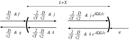
FIG. 16.: Field amplitudes entering and leaving an arm cavity. The cavity’s front-port input and output amplitudes $D$, $f$ and $g$ are defined in Eqs. (B6) and (B8) and Fig. 15, and it’s back-port input $q$ is defined in Eq. (B17).

For pedagogical simplicity, the distance from the beam splitter to the front mirror of each arm cavity is set to an integral multiple of the carrier wavelength and is assumed to be far smaller than $c/\Omega$ (the wavelength associated with the sidebands). This means that there are no net phase shifts of the light in traveling between the beam splitter and the cavity’s front mirror; i.e., the field amplitudes $D/\sqrt{2}\;\&\;f$ (or $D/\sqrt{2}\;\&\;g$) arriving at (or departing from) the mirror are the same as those departing from (or arriving at) the beam splitter; cf. Figs. 16 and 15.

The cavity’s length is adjusted to an integral number of carrier wavelengths so there is no carrier phase shift from one end of the cavity to the other, and inside the cavity the carrier amplitude is amplified by the standard resonance factor $2/\sqrt{T}$. (Losses are small enough to be of little importance for the carrier.) Because the side bands inside the cavity have a frequency dependence $g_{j}e^{-i\Omega t}\cos(\omega_{o}t)$ at the front mirror location [cf. Eq. (B5)], they propagate down the cavity as $g_{j}e^{-i\Omega(t-z)}\cos[\omega_{o}(t-z)]$ and upon reaching the back mirror (where $cos[\omega_{o}(t-z)]=\cos[\omega t]$), they have acquired the phase shift indicated in the figure, $g_{j}e^{i\Omega L/c}$; and similarly for the $k_{j}$ field propagating in the other direction.

The standard junction conditions at the front mirror imply that

$$j_{j}=\sqrt{T}f_{j}+\sqrt{R}k_{j}\;,\quad g_{j}=-\sqrt{R}f_{j}+\sqrt{T}k_{j}\;.$$ (B12)

We denote by $X(t)$ the change of arm length produced by radiation pressure and the gravitational waves, and by $X$ its Fourier transform. The oscillating $X(t)$ pumps carrier light into the side bands. More specifically, in traveling from the front mirror $z=0$ to the perturbed position $z=L+X(t)$ of the back mirror, then reflecting and propagating to the unperturbed location $z=L$, the carrier field acquires the form

$$E_{\rm carrier}=\sqrt{4\pi\hbar\omega_{o}\over{\cal A}c}\sqrt{2\over T}\sqrt{2}D\cos\left(\omega_{o}[t-2X(t)/c]\right)$$ (B13)

$$=\sqrt{4\pi\hbar\omega_{o}\over{\cal A}c}\sqrt{4\over T}D\left(\cos\omega_{o}t+\sin\omega_{o}t{2\omega_{o}\over c}\int_{-\infty}^{+\infty}Xe^{-i\Omega t}{d\Omega\over 2\pi}\right)$$ (B14)

(B15)

Comparing with the standard expression for the field at the location of the unperturbed end mirror [Eq. (B5) with the amplitude changes indicated in the lower right of Fig. 16, $D\rightarrow(2/\sqrt{2})(D/\sqrt{2})$ and $d_{j}\rightarrow k_{j}e^{-i\Omega L/c}$], we obtain the following expression for the field fed from the carrier $D$ into the sideband amplitudes $k_{j}$:

$$\delta k_{1}=0\;,\quad\delta k_{2}={2\over\sqrt{T}}D{2\omega_{o}\over c}X\;.$$ (B16)

This acts as a source term in the standard junction condition for the back mirror:

$$k_{j}e^{-i\Omega L/c}=\sqrt{\tilde{R}}j_{j}e^{i\Omega L/c}+\sqrt{\tilde{T}}q_{j}+\delta k_{j}\;.$$ (B17)

Note that $q_{j}$ is the noise-producing vacuum fluctuation that leaks into the cavity as a result of the optical losses.

3 Cavity’s internal field and radiation-pressure fluctuations

By combining the front-mirror and back-mirror junction conditions (B12) and (B17) we obtain for the side-band amplitude in the cavity

$$j_{j}={\sqrt{T}f_{j}+\sqrt{R}e^{i\Omega L/c}\left(\sqrt{\tilde{T}}\;q_{j}+\delta k_{j}\right)\over 1-\sqrt{R\tilde{R}}e^{2i\Omega L/c}}\;.$$ (B18)

Equations (B11) and $\sqrt{R}=\sqrt{1-T}=\sqrt{1-0.033}\simeq 1$ allow us to make the approximations $\sqrt{R}e^{i\Omega L/c}\simeq 1$ in the numerator and [using (17)]

$$1-\sqrt{R\tilde{R}}e^{2i\Omega L/c}\simeq(2L/c)(\gamma_{*}-i\Omega)\;,\$$ (B19)

$$\gamma_{*}\equiv\gamma(1+\epsilon/2)$$ (B20)

in the denominator (accurate to better than 1 per cent for all $\Omega$ of interest to us), thereby bringing Eq. (B18) into the form

$$j_{j}={\sqrt{T}(f_{j}+\sqrt{\epsilon/2}\;q_{j})+\delta k_{j}\over(2L/c)(\gamma_{*}-i\Omega)}\;,$$ (B21)

where we have used $\tilde{T}={1\over 2}\epsilon T$. The cavity’s internal electric field $E_{\rm int}$ is expression (B5) with $D\rightarrow(2/\sqrt{T})(D/\sqrt{2})$ [Eq. (B15)] and $d_{j}\rightarrow j_{j}$ [expression (B21)]; cf. Fig. 16. The power circulating in the cavity is this $(\overline{E_{\rm int}^{2}}/4\pi){\cal A}c$, and consists of two parts, a steady classical piece

$$W_{\rm circ}={1\over 2}{4D^{2}\over T}\hbar\omega_{o}={2\over T}I_{o}={I_{o}/2\over\gamma L/c}\;,$$ (B22)

and a fluctuating piece

$$\delta W_{\rm circ}=\int_{0}^{\infty}{\sqrt{I_{o}\hbar\omega_{o}}(f_{1}+\sqrt{\epsilon/2}\;q_{1})\over(L/c)(\gamma_{*}-i\Omega)}e^{-i\Omega t}{d\Omega\over 2\pi}+{\rm HC}\;,$$ (B23)

where HC means Hermitian conjugate (adjoint) of the previous term.

4 Mirror motion

The circulating-power fluctuations (B23) produce a fluctuating radiation-pressure (back-action) force

$$F_{\rm BA}=2\delta W_{\rm circ}/c$$ (B24)

on each mirror. This force is equal and opposite on the cavity’s two mirrors and, along with the gravitational waves, it produces the following acceleration of the mirror separation:

$${d^{2}X(t)\over dt^{2}}={1\over 2}\eta_{ne}L{d^{2}h(t)\over dt^{2}}+{4\delta W_{\rm circ}(t)\over mc}\;.$$ (B25)

Here $h(t)$ is the gravitational-wave field (projected onto the interferometer’s arms), and $\eta_{ne}$ is $+1$ for the north arm and $-1$ for the east arm (one arm is stretched while the other is squeezed).

Below we will need an expression for the (Fourier transform of the) arm-length difference, $x=X_{n}-X_{e}$. It can be obtained by Fourier transforming the equation of motion (B25), solving for $X$ (i.e., $X_{n}$ or $X_{e}$), inserting expression (B23) for $\delta W_{\rm circ}$, and then taking the difference of the north and east arms. The result is

$$x=Lh+x_{\rm BA}$$ (B26)

[cf. Eq. (21)], where

$$x_{\rm BA} = {-4\sqrt{2I_{o}\hbar\omega_{o}}\;(a_{1}+\sqrt{\epsilon/2}\;n_{1})\over m\Omega^{2}L(\gamma_{*}-i\Omega)}$$ (B27)

$$= -\sqrt{{\cal K}_{*}/2}\;Lh_{\rm SQL}(a_{1}+\sqrt{\epsilon/2}\;n_{1})e^{i\beta_{*}}\;,$$ (B28)

Here we have introduced the quadrature amplitude for the difference of the arms’ noise fields

$$n_{j}\equiv{q_{j}^{n}-q_{j}^{e}\over\sqrt{2}}\;$$ (B29)

and have used Eq. (B8) for $f_{1}^{n}$ and $f_{1}^{e}$, and Eqs. (133), (132), (26) and (27) for the coupling constant ${\cal K}_{*}$, the phase $\beta_{*}$, the SQL power $I_{\rm SQL}$ and the standard quantum limit $h_{\rm SQL}$.

Below we shall also need the following expression for the difference of the two arms’ sideband fields produced by the mirror motions’ coupling to the carrier:

$${\delta k_{2}^{n}-\delta k_{2}^{e}\over\sqrt{2}}={2\sqrt{2}\over\sqrt{T}}\sqrt{I_{o}\over\hbar\omega_{o}}{\omega_{o}x\over c}\;.$$ (B30)

This follows from Eqs. (B16), (B6) and (18)

5 Cavity output

The field exiting from the (north or east) cavity is obtained by combining Eqs. (B12), (B17) and (B18):

$$g_{j}={\sqrt{\tilde{R}}e^{2i\Omega L/c}-\sqrt{R}\over 1-\sqrt{R\tilde{R}}e^{2i\Omega L/c}}f_{j}+{\left(\sqrt{T\tilde{T}}q_{j}+\sqrt{T}\delta k_{j}\right)e^{i\Omega L/c}\over 1-\sqrt{R\tilde{R}}e^{2i\Omega L/c}}\;.$$ (B31)

Inserting Eq. (B19) for the denominator and analogous expressions for the numerator, and discarding terms that are higher order than linear in the losses, we bring Eq. (B31) into the form

$$g_{j}=\left(1-{1\over 2}{\cal E}\right)e^{2i\beta}f_{j}+\sqrt{\cal E}e^{i\beta}q_{j}+\sqrt{(c/2L)^{2}T\over\gamma_{*}^{2}+\Omega^{2}}e^{i\beta_{*}}\delta k_{j}\;,$$ (B32)

where $\beta_{*}$ is given by Eq. (132).

6 Beam splitter output

By combining Eqs. (B8), (B32), and (B29), we obtain for the dark-port output of the beam splitter

$$b_{j} = \left(1-{1\over 2}{\cal E}\right)a_{j}e^{2i\beta}+\sqrt{\cal E}n_{1}e^{i\beta}$$ (B34)

$$+\sqrt{(c/2L)^{2}T\over\gamma_{*}^{2}+\Omega^{2}}\left({\delta k_{j}^{n}-\delta k_{j}^{e}\over\sqrt{2}}\right)e^{i\beta_{*}}\;.$$

Inserting $\delta k_{1}^{n,e}=0$ [Eq. (B16)] and our expression (B30) for the difference of the $\delta k_{2}$’s, and inserting Eqs. (B26) for $x$ and (133), (27), (B20) for ${\cal K}_{*}$, $h_{\rm SQL}$, $\gamma_{*}$, we obtain for the output fields:

$$b_{1} = \left(1-{1\over 2}{\cal E}\right)a_{1}e^{2i\beta}+\sqrt{\cal E}n_{1}e^{i\beta}\;,$$ (B36)

$$b_{2} = \left(1-{1\over 2}{\cal E}\right)a_{2}e^{2i\beta}+\sqrt{\cal E}n_{2}e^{i\beta}$$ (B38)

$$+\sqrt{2{\cal K}_{*}}\left({h+x_{\rm BA}/L\over h_{\rm SQL}}\right)e^{i\beta_{*}}\;.$$

By inserting expression (B28) for the back-action-induced mirror displacement $x_{\rm BA}$, we obtain the input-output relations quoted in the text: Eqs. (131) and (137) with losses, and Eqs. (23) in the lossless limit

C Filter Parameters

In our discussion of FD homodyne detection [Sec. V], we derived the following requirement for the conventional homodyne phase $\theta$ and the filter parameters $\xi_{J}$ and $\delta_{J}$ (with $J={\rm I}$ and II):

$$\tan\Phi(\Omega) \equiv {\Omega^{2}(\gamma^{2}+\Omega^{2})\over\Lambda^{4}}$$ (C1)

$$= \tan\left(\theta-{\alpha_{{\rm I}+}+\alpha_{{\rm I}_{-}}+\alpha_{{\rm II}+}+\alpha_{{\rm II}_{-}}\over 2}\right)$$ (C2)

[Eqs. (102), (108), and (105)], where

$$\alpha_{J\pm}=\arctan(\xi_{J}\pm\Omega/\delta_{J})\;$$ (C3)

[Eq. (110)]. In this appendix, we shall show that this requirement is satisfied by the parameter choices asserted in the text: Eqs. (107) and (V B).

We initially regard the parameters $\theta$, $\xi_{J}$ and $\delta_{J}$ as unknown. By inserting Eq. (C3) into Eq. (C2) and invoking some trigonometric identities, we obtain the requirement

$${(R_{0}-I_{0}\cot\theta)+(R_{2}-I_{2}\cot\theta)\Omega^{2}+R_{4}\;\Omega^{4}\over(R_{0}\cot\theta+I_{0})+(R_{2}\cot\theta+I_{2})\Omega^{2}+R_{4}\cot\theta\;\Omega^{4}}$$ (C4)

$$={\gamma^{2}\Omega^{2}+\Omega^{4}\over\Lambda^{4}}\;.$$ (C5)

Here $R_{0}+R_{2}\Omega^{2}+R_{4}\Omega^{4}$ is the real part and $I_{0}+I_{2}\Omega^{2}$ is the imaginary part of $(1+i\tan\alpha_{{\rm I}+})(1+i\tan\alpha_{{\rm I}-})(1+i\tan\alpha_{{\rm II}+})(1+i\tan\alpha_{{\rm II}-})$. More specifically,

$$R_{0} = 1-\xi_{\rm I}^{2}-\xi_{\rm II}^{2}-4\xi_{\rm I}\xi_{\rm II}+\xi_{\rm I}^{2}\xi_{\rm II}^{2}\;,$$ (C7)

$$R_{2} = ({1-\xi_{\rm I}^{2})/\delta_{\rm II}^{2}}+({1-\xi_{\rm II}^{2})/\delta_{\rm I}^{2}}\;,$$ (C8)

$$R_{4} = 1/(\delta_{\rm I}^{2}\delta_{\rm II}^{2})\;,$$ (C9)

$$I_{0} = 2(\xi_{\rm I}+\xi_{\rm II})(1-\xi_{\rm I}\xi_{\rm II})\;,$$ (C10)

$$I_{2} = 2\xi_{\rm II}/\delta_{\rm I}^{2}+2\xi_{\rm I}/\delta_{\rm II}^{2}\;.$$ (C11)

To get rid of the $\Omega^{4}$ term in the denominator of Eq. (C5), we must set

$$\theta=\pi/2\;,\quad{\rm so}\cot\theta=0\;.$$ (C12)

(We cannot set $R_{4}=0$ since that would require an infinite bandwidth for one or both of the filters.) To get rid of the $\Omega^{2}$ term in the denominator and the constant term in the numerator, and to make the $\Omega^{2}$ and $\Omega^{4}$ terms in the numerator have the correct coefficients, we must set

$$I_{2} = 0\;,$$ (C14)

$$R_{0} = 0\;,$$ (C15)

$$R_{2}^{2}/(I_{0}R_{4}) = \gamma^{4}/\Lambda^{4}\equiv 4/P\;,$$ (C16)

$$R_{2}/R_{4} = \gamma^{2}\;.$$ (C17)

Here we have used definition (112) of the constant $P$.

Equations (C12) are four equations for the four unkown filter parameters: the fractional frequency offsets $\xi_{\rm I}$, $\xi_{\rm II}$ and the half bandwidths $\delta_{\rm I}$, $\delta_{\rm II}$. In the next four paragraphs we shall explore the consequences of these four equations, arriving finally at the solution (V B) for $\xi_{\rm I}$, $\xi_{\rm II}$, $\delta_{\rm I}$ and $\delta_{\rm II}$ given in the text.

Equation (C14) implies that

$$\delta_{\rm I}^{2}/\delta_{\rm II}^{2}=-\xi_{\rm II}/\xi_{\rm I}\;.$$ (C18)

Equation (C15) implies that $(1-\xi_{\rm I}\xi_{\rm II})^{2}=(\xi_{\rm I}+\xi_{\rm II})^{2}$. It turns out that one of the frequency offsets is positive and the other is negative (cf. Fig. 10); we choose $\xi_{\rm I}$ to be the positive one. It also turns out that $\xi_{\rm I}+\xi_{\rm II}$ is positive (cf. Fig. 10). Consequently, we can take the square root of the above equation to obtain

$$1-\xi_{\rm I}\xi_{\rm II}=\xi_{\rm I}+\xi_{\rm II}\;,$$ (C19)

which enables us to express the frequency offsets in terms of each other:

$$\xi_{\rm I}={1-\xi_{\rm II}\over 1+\xi_{\rm II}}\;,\quad\xi_{\rm II}={1-\xi_{\rm I}\over 1+\xi_{\rm I}}\;.$$ (C20)

Equation (C16), when combined with Eqs. (C18) and (C19), implies that

$${8\over P}={\left[\sqrt{-\xi_{\rm II}\over\xi_{\rm I}}(1-\xi_{\rm I}^{2})+\sqrt{-\xi_{\rm I}\over\xi_{\rm II}}(1-\xi_{\rm II}^{2})\right]^{2}\over(\xi_{\rm I}+\xi_{\rm II})^{2}}\;.$$ (C21)

We shall now combine this equation with Eqs. (C20) to obtain Eqs. (V B) for the frequency offsets $\xi_{\rm I}$ and $\xi_{\rm II}$ in terms of $P=4\gamma^{4}/\Lambda^{4}$. Our first step is to define $A_{\pm}$ by Eqs. (114) and (115), which are equivalent to

$$A_{+}\equiv{\xi_{\rm I}\over\xi_{\rm I}^{2}-1}\;,\quad A_{-}\equiv{\xi_{\rm II}\over\xi_{\rm II}^{2}-1}\;.$$ (C22)

Note that the relation (C20) between $\xi_{\rm I}$ and $\xi_{\rm II}$ is equivalent to

$$4A_{+}A_{-}=1\;.$$ (C23)

By using Eqs. (C20), (C22) and (C23), we can reexpress the right side of Eq. (C21) solely in terms of $A_{+}$:

$${8\over P}={(4A_{+}^{2}-1)^{2}\over A_{+}(4A_{+}^{2}+1)}\;.$$ (C24)

It is convenient to define $Q$ by Eqs. (113), which are equivalent to

$$A_{+}+A_{-}\equiv 2Q/P\;.$$ (C25)

Using Eqs. (C23) and (C25), we can rewrite (C24) in terms of $Q$ instead of $A_{+}$:

$${2\over P}={2Q\over P}-{P\over 2Q}\;,$$ (C26)

which can be solved for $Q$ as a function of $P$

$$Q={1+\sqrt{1+P^{2}}\over 2}\;.$$ (C27)

This is the relation asserted in the text, Eq. (112), and it completes our derivation of Eqs. (112)–(115) for the frequency offsets $\xi_{\rm I}$ and $\xi_{\rm II}$ in terms of $P$.

Turn, finally, to the consequences of Eq. (C17), which says

$$\gamma^{2}=\delta_{\rm I}^{2}(1-\xi_{\rm I}^{2})+\delta_{\rm II}^{2}(1-\xi_{\rm II}^{2})\;.$$ (C28)

By eliminating $\delta_{\rm II}$ with the aid of Eq. (C18), we obtain

$$\gamma^{2}=\delta_{\rm I}^{2}\xi_{\rm I}\left({1-\xi_{\rm I}^{2}\over\xi_{\rm I}}-{1-\xi_{\rm II}^{2}\over\xi_{\rm II}}\right)\;.$$ (C29)

Using Eqs. (C22), (C23), and (113), we can rewrite this as

$${\delta_{\rm I}\over\gamma}=\sqrt{P\over 8\xi_{1}\sqrt{Q}}\;,$$ (C30)

which is the formula for the half bandwidth $\delta_{\rm I}$ given in the text, Eq. (116). The corresponding formula for $\delta_{\rm II}$, Eq. (117), follows directly from Eqs. (C30) and (C18).

REFERENCES

- [1] http://www.ligo.caltech.edu/.
- [2] V. B. Braginsky and F. Ya. Khalili, Rev. Mod. Phys. 68, 1 (1996).
- [3] V. B. Braginsky and F. Ya. Khalili, Quantum Measurement, (Cambridge University Press, Cambridge, 1992). Note: In this reference the spectral densities are double sided and thus are 1/2 the single-sided spectral densities used in the present paper.
- [4] V. B. Braginsky, M. L. Gorodetsky, F. Ya. Khalili, A. B. Matsko, K. S. Thorne, and S. P. Vyatchanin, Phys. Rev. D, submitted; gr-qc/0109003.
- [5] V. B. Braginsky, Sov. Phys.—JETP, 26, 831 (1968); V. B. Braginsky, in Physical Experiments with Test Bodies, NASA Technical Translation TT F-672 (U.S. Technical Information Service, Springfied, VA, 1972).
- [6] V. B. Braginsky and Yu. I. Vorontsov, Sov. Phys.—Uspekhi, 17, 644 (1975).
- [7] E. Gustafson, D. Shoemaker, K. Strain and R. Weiss, LSC White Paper on Detector Research and Development, LIGO Document Number T990080-00-D (Caltech/MIT, 11 September 1999).
- [8] See, e.g., S. Rowan et. al., Phys. Lett. A 233, 303 (1997); V. B. Braginsky, M. L. Gorodetsky and S. P. Vyatchanin, Phys. Lett. A 264, 1 (1999); and references therein.
- [9] For a very general demonstration that MW is the minimum circulating power that is required to beat the standard quantum limit in a wide variety of QND interferometer designs, see V. B. Braginsky, M. L. Gorodetsky, F. Ya. Khalili and K. S. Thorne, in Proceedings of the Third Edoardo Amaldi Meeting on Gravitational Waves, edited by S. Meshkov and V. Kondrashov (AIP Press, Melville, NY), p. 180.
- [10] V. B. Braginsky, M. L. Gorodetsky, F. Ya. Khalili and K. S. Thorne, Phys. Rev. D, 61, 044022 (2000).
- [11] P. Purdue, Phys. Rev. D, in preparation.
- [12] C. M. Caves, K. S. Thorne, R. W. P. Drever, V. D. Sandberg, and M. Zimmermann, Rev. Mod. Phys. 52, 341 (1980); V. B. Braginsky, Yu. I. Vorontsov and K. S. Thorne, Science 209, 547 (1980); C. M. Caves, in Quantum Optics, Experimental Gravity, and Measurement Theory, edited by P. Meystre and M. O. Scully (Plenum, New York, 1982), p. 567. See also W. G. Unruh, Phys. Rev. D 19, 2888 (1979).
- [13] V. B. Braginsky, M. L. Gorodetsky and F. Ya. Khalili, Phys. Lett. A 232, 340 (1997); V. B. Braginsky, M. L. Gorodetsky and F. Ya. Khalili, Phys. Lett. A 246, 485 (1998); V. B. Braginsky and F. Ya. Khalili, Phys. Lett. A 257, 241 (1999).
- [14] W. G. Unruh, in Quantum Optics, Experimental Gravitation, and Measurement Theory, eds. P. Meystre and M. O. Scully, (Plenum, 1982), p. 647.
- [15] V. B. Braginsky and A. B. Manukin, Zh. Teor. Eksp. Fiz. 52, 987 (1967) (Eng. translation: JETP 25, 653 (1967)).
- [16] A similar effect has been considered by A. V. Gusev and V. N. Rudenko, Zh. Eksp. Teor. Fiz. 76, 1488 (1979).
- [17] C. M. Caves, Phys. Rev. D, 23, 1693 (1981),
- [18] M. T. Jaekel and S. Reynaud, Europhys. Lett. 13, 301 (1990).
- [19] A. F. Pace, M. J. Collett and D. F. Walls, Phys. Rev. A 47, 3173 (1993).
- [20] M. Xiao, L.-A. Wu, and H. J. Kimble, Phys. Rev. Lett. 59, 278 (1987).
- [21] P. Grangier, R. E. Slusher, B. Yurke, and A. LaPorta, Phys. Rev. Lett. 59, 2153 (1987).
- [22] See, e.g., the following special issues of journals dealing with squeezing via nonlinear optics: J. Opt. Soc. Am. 4, 1450–1741; and Quantum Noise Reduction in Optical Systems, eds. C. Fabre and E. Giacobino, App. Phys. B 55, 189ff (1992).
- [23] S. P. Vyatchanin and A. B. Matsko, JETP 77, 218 (1993); S. P. Vyatchanin and E. A. Zubova, Phys. Lett. A 203, 269 (1995); S. P. Vyatchanin, Phys. Lett. A, 239, 201 (1998).
- [24] S. P. Vyatchanin and A. B. Matsko, JETP 82, 1007 (1996).
- [25] S. P. Vyatchanin and A. B. Matsko, JETP 83, 690 (1996).
- [26] C. M. Caves and B. L. Schumaker, Phys. Rev. A 31, 3068 (1985).
- [27] B. S. Schumaker and C. M. Caves, Phys. Rev. A 31, 3093 (1985).
- [28] D. F. Walls and G. J. Milburn, Quantum Optics (Springer-Verlag, Berlin, 1994); L. Mandel and E. Wolf, Optical Coherence and Quantum Optics (Cambridge University Press, Cambridge, 1995). Some readers may also find useful background in C. W. Gardiner, Quantum Noise (Springer-Verlag, Berlin, 1991).
- [29] R. W. P. Drever et. al., in P. Meystre and M. O. Scully eds. Quantum Optics, Experimental Gravity and Measurement Theory, (Plenum, New York, 1981), p. 503.
- [30] C. Fabre, M. Pinard, S. Bourzeix, A. Heidmann, E. Giacobino, and S. Reynaud, Phys. Rev. A 49, 1337 (1994); S. Mancini and P. Tombesi, Phys. Rev. A 49, 4055 (1994); A. Heidmann and S. Reynaud, Phys. Rev. A 50, 4237 (1994); M. Pinard, C. Fabre, and A. Heidmann, Phys. Rev. A 51, 2443 (1995).
- [31] H. J. Kimble, in Fundamental Systems in Quantum Optics, Les Houches Session LIII, 1990, edited by J. Dalibard, J. M. Raimond, and J. Zinn-Justin (Elsevier, Amsterdam, 1992), pp. 549–674.
- [32] Y. Chen, private communication.
- [33] For example, although the detected degree of squeezing in L.-A. Wu, M. Xiao and H. J. Kimble, J. Opt. Soc. Am. B, 4, 1465 (1987) was only -4.3 dB, the inferred degree of squeezing was much larger: after making an absolute accounting for passive linear losses, these authors inferred a degree of squeezing corresponding to approximately -12 dB, which provides a benchmark for how well the basis nonlinear optical process of parametric down conversion conforms to simple theoretical models [31]. Somewhat more recently, E. S. Polzik, J. Carri and J. H. Kimble, Appl. Phys. B 55, 279 (1992) have recorded quantum noise reductions of -6 dB directly in the observed homodyne current. In this case the degree of squeezing was limited not by passive linear losses, but instead by nonlinear light induced absorption in the potassium niobate crystal used for parametric down conversion. Quite recently K. Schneider, M. Lang, J. Mlynek and S. Schiller, Optics Express, 2, 59 (1998) have reported 6.5 dB of vacuum squeezing from a below-threshold optical parametric oscillator, with comparable levels reported by P. K. Lam et. al., J. Opt. B – Quant. Semiclass. Opt., 1, 469 (1999).
- [34] Eq. (44) of K. S. Thorne, in 300 Years of Gravitation, edited by S. W. Hawking and W. Israel (Cambridge University Press, Cambridge, 1987).
- [35] P. R. Saulson, Phys. Rev. D, 42, 2437 (1990).
- [36] V. B. Braginsky, V. P. Mitrofanov, and K. V. Tokmakov, Phys. Lett. A, 218, 164 (1996); K. Tokmakov, V. Mitrofanov, V. Braginsky, S. Rowan and J. Hough, in Proceedings of the Third Amaldi Conference on Gravitational Waves, edited by S. Meshkov and V. Kondrashov (AIP Press, Melville, NY), p. 445.
- [37] For analyses of the compatibility of input squeezing, modulations, and and signal recycling, see S. Song, Recycling and Squeezing in High-Precision Optical Measurements, unpublished PhD thesis, University of Southern California (1994); and J. Geabanacloche and G. Leuchs, J. Mod. Opt., 34, 793 (1987).
- [38] J. Mizuno, K. A. Strain, P. G. Nelson, J. M. Chen, R. Schilling, A. Rudiger, W. Winkler, and K. Danzmann, Phys. Lett. A 175, 273 (1993).
- [39] Equation (191) can be derived by the techniques used in Ref. [25]; see especially Eqs. (13)–(15) of [25].
- [40] The experimental challenge simply to reach the SQL for mirror position is daunting. Two recent experiments that addressed this challenge with small masses but were impeded by thermal noise are reported in Refs. [42] and [43].
- [41] A. Dorsel, J. D. McCullen, P. Meystre, E. Vignes, and H. Walther, Phys. Rev. Lett. 51, 1550 (1983).
- [42] Y. Hadjar, P. F. Cohadon, C. J. Aminoff, M. Pinard, and A. Heidmann, Europhys. Lett. 47, 545 (1999).
- [43] I. Tittonen et. al., Phys. Rev. A 59, 1038 (1999);
- [44] K. Jacobs, I. Tittonen, H. M. Wiseman, and S. Schiller, Phys. Rev. A 60, 538 (1999).
- [45] For a detailed discussion of losses and various efficiency factors associated with the spatial overlap of fields in interferometry with squeezed light, see Min Xiao, unpublished PhD thesis, University of Texas at Austion (1988), Chap. 4, Sec. IIA.
- [46] Equation (14) of Appendix C of A. E. Siegman, An Introduction to Lasers and Masers (McGraw-Hill, New York, 1971).