Superfluid analogies of cosmological phenomena

Abstract

In a modern viewpoint the relativistic quantum field theory is the emergent phenomenon arising in the low energy corner of the physical fermionic vacuum – the medium, whose nature remains unknown. The same phenomenon occurs in the condensed matter systems: In the extreme limit of low energy the condensed matter system of special universality class acquires all the symmetries, which we know today in high energy physics: Lorentz invariance, gauge invariance, general covariance, etc. The chiral fermions as well as gauge bosons and gravity field arise as fermionic and bosonic collective modes of the system. The inhomogeneous states of the condensed matter ground state – vacuum – induce nontrivial effective metrics of the space, where the free quasiparticles move along geodesics. This conceptual similarity between condensed matter and quantum vacuum allows us to simulate many phenomena in high energy physics and cosmology, including axial anomaly, baryoproduction and magnetogenesis, event horizon and Hawking radiation, cosmological constant and rotating vacuum, etc., probing these phenomena in ultra-low-temperature superfluid helium, atomic Bose condensates and superconductors. Some of the experiments have been already conducted.

Contents

toc

I Introduction. Physical vacuum as condensed matter.

The traditional Grand Unification view is that the low-energy symmetry of our world is the remnant of a larger symmetry, which exists at high energy and is broken, when the energy is reduced. According to this philosophy the higher the energy the higher is the symmetry: $U(1)\times SU(3)\rightarrow U(1)\times SU(2)\times SU(3)\rightarrow SO(10)\rightarrow$supersymmetry, etc. The less traditional view is quite opposite: it is argued that starting from some energy scale one probably finds that the higher the energy the poorer are the symmetries of the physical laws, and finally even the Lorentz invariance and gauge invariance will be smoothly violated [1, 2]. From this point of view the relativistic quantum field theory is an effective theory [3, 4]. It is an emergent phenomenon arising as a fixed point in the low energy corner of the physical vacuum. In the vicinity of the fixed point the system acquires new symmetries which it did not have at higher energy. And it is quite possible that even such symmetries as Lorentz symmetry and gauge invariance are not fundamental, but gradually appear when the fixed point is approached.

Both scenaria are supported by the condensed matter systems. In particular, superfluid ³He-A provides an instructive example of both ways of the behavior of the symmetry. At high temperature the ³He gas and at lower temperature the ³He liquid have all the symmetries, which the ordinary condensed matter can have: translational invariance, global $U(1)$ group and global $SO(3)$ symmetries of spin and orbital rotations. When the temperature decreases further the liquid ³He reaches the superfluid transition temperature $T_{c}$, below which it spontaneously looses all its symmetries except for the translational one – it is still liquid. This breaking of symmetry at low temperature and thus at low energy reproduces the Grand Unification scheme, where the symmetry breaking is the most important component.

However, this is not the whole story. When the temperature is reduced further the opposite “anti-grand-unification” scheme starts to work: in the limit $T\rightarrow 0$ the superfluid ³He-A gradually acquires from nothing almost all the symmetries, which we know today in high energy physics: (analog of) Lorentz invariance, local gauge invariance, elements of general covariance, etc. It appears that such an enhancement of symmetry in the limit of low energy happens because ³He-A belongs to a special universality class of Fermi systems [5]. For the condensed matter of such class the chiral fermions as well as gauge bosons and gravity field arise as fermionic and bosonic collective modes together with the chirality itself and with corresponding symmetries. The inhomogeneous deformations of the condensed matter ground state – quantum vacuum – induce nontrivial effective metrics of the space, where the free quasiparticles move along geodesics. This conceptual similarity between condensed matter and quantum vacuum gives some hint on the origin of symmetries and also allows us to simulate many phenomena in high energy physics and cosmology.

The quantum field theory, which we have now, is incomplete due to ultraviolet diveregences at small scales. The crucial example is provided by the quantum theory of gravity, which after 70 years of research is still far from realization in spite of numerous beautiful achievements [6]. This is a strong indication that the gravity, both classical and quantum, is not fundamental: It is effective field theory which is not applicable at small scales, where the “microscopic” physics of vacuum becomes important and according to the “anti-grandunification” scenario some or all of the known symmetries in Nature are violated. The analogy between quantum vacuum and condensed matter could give an insight into this transPlanckian physics since it provides examples of the physically imposed deviations from Lorentz and other invariances at higher energy. This is important in many different areas of high energy physics and cosmology, including possible CPT violation and black holes, where the infinite red shift at the horizon opens the route to the transPlanckian physics.

The condensed matter teaches us that the low-energy properties of different condensed matter vacua (magnets, superfluids, crystals, superconductors, etc.) are robust, i.e. they do not depend much on the details of microscopic (atomic) structure of these substances. The main role is played by symmetry and topology of condensed matter: they determine the soft (low-energy) hydrodynamic variables, the effective Lagrangian describing the low-energy dynamics, topological defects and quantization of physical parameters. The microscopic details provide us only with the “fundamental constants”, which enter the effective phenomenological Lagrangian, such as speed of “light” (say, the speed of sound), superfluid density, modulus of elasticity, magnetic susceptibility, etc. Apart from these “fundamental constants”, which can be rescaled, the systems behave similarly in the infrared limit if they belong to the same universality and symmetry classes, irrespective of their microscopic origin.

The detailed information on the system is lost in such acoustic or hydrodynamic limit [7]. From the properties of the low energy collective modes of the system – acoustic waves in case of crystals – one cannot reconstruct the atomic structure of the crystal since all the crystals have similar acoustic waves described by the same equations of the same effective theory, in crystals it is the classical theory of elasticity. The classical fields of collective modes can be quantized to obtain quanta of acoustic waves – the phonons. This quantum field remains the effective field which is applicable only in the long-wave-length limit, and does not give a detailed information on the real quantum structure of the underlying crystal (exept for its symmetry class). In other words one cannot construct the full quantum theory of real crystal using the quantum theory of elasticity. Such theory would always contain divergencies on atomic scale, which cannot be regularized.

The same occurs in other effective theories of condensed matter. In particular the naive approach to calculate the ground state (vacuum) energy of superfluid liquid ⁴ using the zero point energy of phonons gives even the wrong sign of the vacuum energy, as we shall see in Sec. II G.

It is quite probable that in the same way the quantization of classical gravity, which is one of the infrared collective modes of quantum vacuum, will not add more to our understanding of the “microscopic” structure of the vacuum [8, 9, 7]. Indeed, according to this “anti-grandunification” analogy, such properties of our world, as gravitation, gauge fields, elementary chiral fermions, etc., all arise in the low energy corner as a low-energy soft modes of the underlying “condensed matter”. At high energy (of the Planck scale) these modes merge with the continuum of the all high-energy degrees of freedom of the “Planck condensed matter” and thus cannot be separated anymore from each other. Since the gravity is not fundamental, but appears as an effective field in the infrared limit, the only output of its quantization would be the quanta of the low-energy gravitational waves – gravitons. The more deep quantization of gravity makes no sense in this phylosophy. In particular, the effective theory cannot give any prediction for the vacuum energy and thus for the cosmological constant.

The main advantage of the condensed matter analogy is that in principle we know the condensed matter structure at any relevant scale, including the interatomic distance, which plays the part of one of the Planck length scales in the hierarchy of scales. Thus the condensed matter can suggest possible routes from our present low-energy corner of “phenomenology” to the “microscopic” physics at Planckian and trans-Planckian energies. It can also show the limitation of the effective theories: what quantities can be calculated within the effective field theory using, say, renormalization group approach, and what qantities depend essentially on the details of the transPlanckian physics.

In the main part of the review we consider superfluid ³He in its A-phase, which belongs the special class of Fermi liquids, where the effective gravity, gauge fields and chiral fermions appear in the low-energy corner together with Lorentz and gauge invariance [5, 10], and discuss the correspondence between the phenomena in superfluid ³He-A and that in relativistic particle physics. However, some useful analogies can be provided even by Bose liquid – superfluid ⁴He, where a sort of the effective gravitational field appears in the low energy corner. That is why it is instructive to start with the simplest effective field theory of Bose superfluid which has a very restricted number of effective fields.

II Landau-Khalatnikov two-fluid hydrodynamics as effective theory of gravity.

A Superfluid vacuum and quasiparticles.

According to Landau and Khalatnikov [11] a weakly excited state of the collection of interacting ⁴He atoms can be considered as a small number of elementary excitations – quasiparticles (phonons and rotons). In addition, the state without excitation – the ground state or vacuum – can have collective degrees of freedom. The superfluid vacuum can move without friction, and inhomogeneity of the flow serves as the gravitational and/or other effective fields. The matter propagating in the presence of this background is represented by fermionic (in Fermi superfluids) or bosonic (in Bose superfluids) quasiparticles, which form the so called normal component of the liquid. Such two-fluid hydrodynamics introduced by Landau and Khalatnikov [11] is the example of the effective field theory which incorporates the motion of both the superfluid background (gravitational field) and its excitations (matter). This is the counterpart of the Einstein equations, which incorporate both gravity and matter.

One must distinguish between the bare particles and quasiparticles in superfluids. The particles are the elementary objects of the system on a microscopic “transPlanckian” level, these are the atoms of the underlying liquid (³He or ⁴He atoms). The many-body system of the interacting atoms form the quantum vacuum – the ground state. The nondissipative collective motion of the superfluid vacuum with zero entropy is determined by the conservation laws experienced by the atoms and by their quantum coherence in the superfluid state. The quasiparticles are the particle-like excitations above this vacuum state. The bosonic excitations in superfluid ⁴He and fermionic and bosonic excitations in superfluid ³He form the viscous normal component of these liquids, which correspond to matter in our analogy. The normal component is responsible for the thermal and kinetic low-energy properties of superfluids.

B Dynamics of superfluid vacuum.

In the simplest superfluid the coherent motion of the superfluid vacuum is characterized by two collective (hydrodynamic) variables: the particle number density $n({\bf r},t)$ of atoms comprising the liquid and superfluid velocity ${\bf v}_{\rm s}({\bf r},t)$ of their coherent motion. In superfluid ⁴He the superfluid velocity is the gradient of the phase of the order parameter (${\bf v}_{\rm s}=(\hbar/m)\nabla\Phi$, where $m$ is the bare mass of particle – the mass of ⁴He atom) and thus the flow of vacuum is curl-free: $\nabla\times{\bf v}_{\rm s}=0$. This is not however a rule: as we shall see in Sec. V A 3 the superfluid vacuum flow of ³He-A can have a continuous vorticity, $\nabla\times{\bf v}_{\rm s}\neq 0$.

The particle number conservation provides one of the equations of the effective theory of superfluids – the continuity equation:

$${\partial n\over\partial t}+\nabla\cdot{\bf J}=0~{}.$$ (1)

In a strict microscopic theory of monoatomic lquid, $n$ and the particle current ${\bf J}$ are given by the particle distribution function $n({\bf p})$:

$$n=\sum_{\bf p}n({\bf p})~{}~{},~{}~{}{\bf J}={1\over m}\sum_{\bf p}{\bf p}n({\bf p})~{}.$$ (2)

The liquids considered here are nonrelativistic and obeying the Galilean transformation law. In the Galilean system the momentum of particles and the particle current are related by the second Eq.(2).

The particle distribution function $n({\bf p})$ is typically rather complicated function of momentum even at $T=0$ because of the strong interaction between the bare atoms in a real liquid. $n({\bf p})$ can be determined only in a fully microscopic theory and thus never enters the effective theory of superfluidity. The latter instead is determined by quasiparticle distribution function $f({\bf p})$, which is simple because at low $T$ the number of quasiparticles is small and their interaction can be neglected. That is why in equilibrium $f({\bf p})$ given by the thermal Bose distribution (or by the Fermi distribution for fermionic quasiparticles) and in nonequilibrium it can be found from the conventional kinetic equation for quasiparticles.

In the effective theory the particle current has two contributions

$${\bf J}=n{\bf v}_{\rm s}+{\bf J}_{\rm q}~{},~{}{\bf J}_{\rm q}={1\over m}{\bf P}~{},~{}{\bf P}\sum_{\bf p}{\bf p}f({\bf p})~{}.$$ (3)

The first term $n{\bf v}_{\rm s}$ is the current transferred coherently by the collective motion of superfluid vacuum with the superfluid velocity ${\bf v}_{\rm s}$. In equilibrium at $T=0$ this is the only current, but if quasiparticles are excited above the ground state, their momentum ${\bf P}$ gives an additional contribution to the particle current providing the second term in Eq.(3). Note that under the Galilean transformation to the coordinate system moving with the velocity ${\bf u}$, at which the superfluid velocity transforms as ${\bf v}_{\rm s}\rightarrow{\bf v}_{\rm s}+{\bf u}$, the momenta of particle and quasiparticle transform differently: ${\bf p}\rightarrow{\bf p}+m{\bf u}$ for microscopic particles (atoms) and ${\bf p}\rightarrow{\bf p}$ for quasiparticles. The latter occurs because the quasiparticle in effective low-energy theory has no information on such characteristic of the transPlanckian world as the mass of the bare atoms comprising the vacuum state.

The second equation for the collective variables is the London equation for the superfluid velocity, which is curl-free in superfluid ⁴He ($\nabla\times{\bf v}_{\rm s}=0$):

$$m{\partial{\bf v}_{(s)}\over\partial t}+\nabla{\delta{\cal E}\over\delta n}=0~{}.$$ (4)

Together with the kinetic equation for the quasiparticle distribution function $f({\bf p})$, the Eqs.(4) and (1) for collective fields ${\bf v}_{\rm s}$ and $n$ give the complete effective theory for the kinetics of quasiparticles (matter) and coherent motion of vacuum (gravitational field) if the energy functional ${\cal E}$ is known. In the limit of low temperature, where the density if thermal quasiparticles are small, the interaction between quasiparticles can be neglected. Then the simplest Ansatz satisfying the Galilean invariance is

$${\cal E}=\int d^{3}r\left({m\over 2}n{\bf v}_{\rm s}^{2}+\epsilon(n)-\mu n+\sum_{\bf p}\tilde{E}({\bf p},{\bf r})f({\bf p},{\bf r})\right)~{}.$$ (5)

Here $\epsilon(n)$ (or $\tilde{\epsilon}(n)=\epsilon(n)-\mu n$) is the vacuum energy density as a function of the particle density; $\mu$ is the overall constant chemical potential, which is the Lagrange multiplier responsible for the conservation of the total number $N=\int d^{3}x~{}n$ of the ⁴He atoms; $\tilde{E}({\bf p},{\bf r})=E({\bf p},n({\bf r}))+{\bf p}\cdot{\bf v}_{\rm s}({\bf r})$ is the Doppler shifted quasiparticle energy in the laboratory frame with $E({\bf p},n({\bf r}))$ being the quasiparticle energy measured in the frame comoving with the superfluid vacuum.

1 Absence of canonical Lagrangian formalism in effective theories.

The Eqs. (1) and (4) can be obtained from the Hamiltonian formalism using the energy in Eq.(5) as Hamiltonian and the following Poisson brackets

$$\left\{{\bf v}_{\rm s}({\bf r}_{1}),n({\bf r}_{2})\right\}={1\over m}\nabla\delta({\bf r}_{1}-{\bf r}_{2})~{},~{}\left\{n({\bf r}_{1}),n({\bf r}_{2})\right\}=\left\{{\bf v}_{\rm s}({\bf r}_{1}),{\bf v}_{\rm s}({\bf r}_{2})\right\}=0~{}.$$ (6)

The Poisson brackets between components of superfluid velocity are zero only for curl-free superfluidity. In a general case it is

$$\left\{v_{{\rm s}i}({\bf r}_{1}),v_{{\rm s}j}({\bf r}_{2})\right\}=-{1\over mn}e_{ijk}(\nabla\times{\bf v}_{\rm s})_{k}\delta({\bf r}_{1}-{\bf r}_{2})~{}.$$ (7)

In this case even at $T=0$, when the quasiparticles are absent, the Hamiltonian description of the hydrodynamics is only possible: There is no Lagrangian, which can be expressed in terms of the hydrodynamic variables ${\bf v}_{\rm s}$ and $n$. The absence of the Lagrangian in many condensed matter systems is one of the consequences of the reduction of the degrees of freedom in effective field theory, as compared with the fully microscopic description [12]. In ferromagnets, for example, the number of the hydrodynamic variables is odd: 3 components of the magnetization vector ${\bf M}$. They thus cannot form the canonical pairs of conjugated variables. As a result one can use either the Hamiltonian description or introduce the effective action with the Wess-Zumino term, which contains an extra coordinate $\tau$:

$$S_{\rm WZ}\propto\int d^{3}x~{}dt~{}d\tau~{}{\bf M}\cdot(\partial_{t}{\bf M}\times\partial_{\tau}{\bf M})~{}.$$ (8)

According to the analogy the presence of the Wess-Zumino term in the relativistic quantum field theory would indicate that such theory is effective.

C Normal component – “matter”.

In a local thermal equilibrium the distribution of quasiparticles is characterized by local temperature $T$ and by local velocity of the quasiparticle gas ${\bf v}_{\rm n}$, which is called the normal component velocity:

$$f_{\cal T}({\bf p})=\left(\exp{\tilde{E}({\bf p})-{\bf p}{\bf v}_{n}\over T}\pm 1\right)^{-1}~{},$$ (9)

where the sign + is for the fermionic quasiparticles in Fermi superfluids and the sign - is for the bosonic quasiparticles in Bose superfluids. Since $\tilde{E}({\bf p})=E({\bf p})+{\bf p}\cdot{\bf v}_{\rm s}$, the equilibrium distribution is determined by the Galilean invariant quantity ${\bf v}_{\rm n}-{\bf v}_{\rm s}\equiv{\bf w}$, which is the normal component velocity measured in the frame comoving with superfluid vacuum. It is called the counterflow velocity. In the limit when the conterflow velocity ${\bf v}_{\rm n}-{\bf v}_{\rm s}$ is small, the quasiparticle (“matter”) contribution to the liquid momentum and thus to the particle current is proportional to the counterflow velocity:

$$J_{{\rm q}i}=n_{{\rm n}ik}(v_{{\rm n}k}-v_{{\rm s}k})~{},~{}n_{{\rm n}ik}=-\sum_{\bf p}{p_{i}p_{k}\over m}~{}{\partial f_{\cal T}\over\partial E}~{}~{},$$ (10)

where the tensor $n_{{\rm n}ik}$ is the so called density of the normal component. In this linear regime the total current in Eq.(3) can be represented as the sum of the currents carried by the normal and superfluid components

$$J_{i}=n_{{\rm s}ik}v_{{\rm s}k}+n_{{\rm n}ik}v_{{\rm n}k}~{},$$ (11)

where tensor $n_{{\rm s}ik}=n\delta_{ik}-n_{{\rm n}ik}$ is the so called density of superfluid component. In the isotropic superfluids, ⁴He and ³He-B, the normal component density is an isotropic tensor, $n_{{\rm n}ik}=n_{{\rm n}}\delta_{ik}$, while in anisotropic superfluid ³He-A the normal component density is a uniaxial tensor [13]. At $T=0$ the quasiparticles are frozen out and one has $n_{{\rm n}ik}=0$ and $n_{{\rm s}ik}=n\delta_{ik}$ in all monoatomic superfluids.

D Quasiparticle spectrum and effective metric

The structure of the quasiparticle spectrum in superfluid ⁴He becomes more and more universal the lower the energy. In the low energy corner the spectrum of these quasiparticles, phonons, can be obtained in the framework of the effective theory. Note that the effective theory is unable to describe the high-energy part of the spectrum – rotons, which can be determined in a fully microscopic theory only. On the contrary, the spectrum of phonons is linear, $E({\bf p},n)\rightarrow c(n)|{\bf p}|$, and only the “fundamental constant” – the speed of “light” $c(n)$ – depends on the physics of the higher energy hierarchy rank. Phonons represent the quanta of the collective modes of the superfluid vacuum, sound waves, with the speed of sound obeying $c^{2}(n)=(n/m)(d^{2}\epsilon/dn^{2})$. All other information on the microscopic atomic nature of the liquid is lost. Note that for the curl-free superfluids the sound waves represent the only “gravitational” degree of freedom. The Lagrangian for these “gravitational waves” propagating above the smoothly varying background is obtained from equations (1) and (4) at $T=0$ by decomposition of the superfluid velocity and density into the smooth and fluctuating parts: ${\bf v}_{\rm s}={\bf v}_{\rm s~{}~{}smooth}+\nabla\alpha$ [14, 15]. The quadratic part of the Lagrangian for the scalar field $\alpha$ is [16]:

$${\cal L}={m\over 2}n\left((\nabla\alpha)^{2}-{1\over c^{2}}\left(\dot{\alpha}+({\bf v}_{\rm s}\cdot\nabla)\alpha\right)^{2}\right)\equiv{1\over 2}\sqrt{-g}g^{\mu\nu}\partial_{\mu}\alpha\partial_{\nu}\alpha~{}.$$ (12)

The quadratic Lagrangian for sound waves has necessarily the Lorentzian form, where the effective Riemann metric experienced by the sound wave, the so called acoustic metric, is simulated by the smooth parts of the hydrodynamic fields:

$$g^{00}=-{1\over mnc}~{},~{}g^{0i}=-{v_{\rm s}^{i}\over mnc}~{},~{}g^{ij}={c^{2}\delta^{ij}-v_{\rm s}^{i}v_{\rm s}^{j}\over mnc}~{},$$ (13)

$$g_{00}=-{mn\over c}(c^{2}-{\bf v}_{\rm s}^{2})~{},~{}g_{0i}=-{mnv_{{\rm s}i}\over c}~{},~{}g_{ij}={mn\over c}\delta_{ij}~{},~{}\sqrt{-g}={m^{2}n^{2}\over c}~{}.$$ (14)

Here and further ${\bf v}_{\rm s}$ and $n$ mean the smooth parts of the velocity and density fields. Phonons in superfluids and crystals provide a typical example of how an enhanced symmetry and effective Lorentzian metric appear in condensed matter in the low energy corner.

The energy spectrum of sound wave quanta, phonons, which represent the “gravitons” in this effective gravity, is determined by

$$g^{\mu\nu}p_{\mu}p_{\nu}=0~{},~{}~{}{\rm or}~{}~{}(\tilde{E}-{\bf p}\cdot{\bf v}_{\rm s})^{2}=c^{2}p^{2}~{}.$$ (15)

E Effective metric for bosonic collective modes in other systems.

The effective action in Eq.(12) is typical for the low energy collective modes in ordered systems. The more general case is provided by the Lagrangian for the Goldstone bosons in antiferromegnets – the spin waves. The spin wave dynamics in $x-y$ antiferromagnets and in ³He-A is governed by the Lagrangian for the Goldstone variable $\alpha$, which is the angle of the antiferromagnetic vector:

$${\cal L}={1\over 2}\eta^{ij}\nabla_{i}\alpha\nabla_{j}\alpha-{1\over 2}\chi\left(\dot{\alpha}+({\bf v}\cdot\nabla)\alpha\right)^{2}\equiv{1\over 2}\sqrt{-g}g^{\mu\nu}\partial_{\mu}\alpha\partial_{\nu}\alpha~{}.$$ (16)

Here the matrix $\eta^{ij}$ is the spin rigidity; $\chi$ is the spin susceptibility; and ${\bf v}$ is the local velocity of crystall in antiferromagnets and superfluid velocity, ${\bf v}={\bf v}_{\rm s}$, in ³He-A. In antiferromagnets these 10 coefficients give rise to all ten components of the effective Riemann metric:

$$g^{00}=-(\eta\chi)^{1/2}~{},~{}g^{0i}=-(\eta\chi)^{1/2}v^{i}~{},~{}g^{ij}=\left({\eta\over\chi}\right)^{1/2}(\eta^{ij}-\chi v^{i}v^{j})~{},~{}\eta^{-1}={\rm det}(\eta^{ij})~{},$$ (17)

$$g_{00}=-(\eta\chi)^{-1/2}(1-\chi\eta_{ij}v^{i}v^{j})~{},~{}g_{0i}=-\left({\chi\over\eta}\right)^{1/2}\eta_{ij}v^{j}~{},~{}g_{ij}=\left({\chi\over\eta}\right)^{1/2}\eta_{ij}~{},~{}\sqrt{-g}=\left({\chi\over\eta}\right)^{1/2}~{}.$$ (18)

The effective interval is

$$ds^{2}=-{1\over(\eta\chi)^{1/2}}dt^{2}+\left({\chi\over\eta}\right)^{1/2}\eta_{ij}(dx^{i}-v^{i}dt)(dx^{j}-v^{j}dt)~{}.$$ (19)

This form of the interval corresponds to the Arnowitt-Deser-Misner decomposition of the space-time metric, where the function

$$N={1\over(\eta\chi)^{1/4}}~{},$$ (20)

is known as lapse function; $g_{ij}=\left(\chi/\eta\right)^{1/2}\eta_{ij}$ gives the three-metric describing the geometry of space; and the velocity vector ${\bf v}$ plays the part of the so-called shift function (see e.g. the book [17]).

F Effective quantum field and effective action

The effective action in Eq.(12) for phonons and in Eq.(16) for spin waves (magnons) formally obeys the general covariance. In addition, in the classical limit of Eq.(15) corresponding to geometrical optics (in our case this is geometrical acoustics) the propagation of phonons is invariant under the conformal transformation of metric, $g^{\mu\nu}\rightarrow\Omega^{2}g^{\mu\nu}$. This symmetry is lost at the quantum level: the Eq.(12) is not invariant under general conformal transformations, however the reduced symmetry is still there: Eq.(12) is invariant under scale transformations with $\Omega={\rm Const}$.

As we shall see further, in the superfluid ³He-A the other effective fields and new symmetries appear in the low energy corner, including also the effective $SU(2)$ gauge fields and gauge invariance. The symmetry of fermionic Lagrangian induces, after integration over the quasiparticles degrees of freedom, the corresponding symmetry of the effective action for the gauge fields. Moreover, in addition to superfluid velocity field there are appear the other gravitational degrees of freedom with the spin-2 gravitons. However, as distinct from the effective gauge fields, whose effective action is very similar to that in particle physics, the effective gravity cannot reproduce in a full scale the Einstein theory: the effective action for the metric is contaminated by the noncovariant terms, which come from the “transPlanckian” physics [5]. The origin of difficulties with effective gravity in condensed matter is probably the same as the source of the problems related to quantum gravity and cosmological constant.

The quantum quasiparticles interact with the classical collective fields ${\bf v}_{\rm s}$ and $n$, and with each other. In Fermi superfluid ³He the fermionic quasiparticles interact with many collective fields describing the multicomponent order parameter and with their quanta. That is why one obtains the interacting Fermi and Bose quantum fields, which are in many respect similar to that in particle physics. However, this field theory can be applied to a lowest orders of the perturbation theory only. The higher order diagrams are divergent and nonrenormalizable, which simply means that the effective theory is valid when only the low energy/momentum quasiparticles are involved even in their virtual states. This means that only those terms in the effective action can be derived by integration over the quasiparticle degrees of freedom, whose integral are concentrated solely in the low-energy region. For the other processes one must go beyond the effective field theory and consider the higher levels of description, such as Fermi liquid theory, or further the microscopic level of the underlying liquid with atoms and their interactions. In short, all the terms in effective action come from the microscopic “Planck” physics, but only some fraction of them can be derived in a self-consistent way within the effective field theory itself.

In Bose supefluids the fermionic degrees of freedom are absent, that is why the quantum field theory there is too restrictive, but nevertheless it is useful to consider it since it provides the simplest example of the effective theory. On the other hand the Landau-Khalatnikov scheme is rather universal and is easily extended to superfluids with more complicated order parameter and with fermionic degrees of freedom (see the book [13]).

G Vacuum energy and cosmological constant. Nullification of vacuum energy.

The vacuum energy densities $\epsilon(n)$ and $\tilde{\epsilon}(n)=\epsilon(n)-\mu n$, and also the parameters which characterize the quasparticle energy spectrum cannot be determined by the effective theory: they are provided solely by the higher (microscopic) level of description. The vacuum is characterized by the equilibrium value of the particle number density $n_{0}(\mu)$ at given chemical potential $\mu$, which is determined by the minimization of the energy $\tilde{\epsilon}(n)$ which enters the functional in Eq.(5): $d\tilde{\epsilon}/dn=0$. This energy is related to the pressure in the liquid created by external sources provided by the environment. From the definition of the pressure, $P=-d(V\epsilon(N/V))/dV$ where $V$ is the volume of the system and $N$ is the total number of the ⁴He atoms, one obtains that the energy density $\tilde{\epsilon}(n)=\epsilon(n)-\mu n$ of the vacuum in equilibrium and the vacuum pressure are related in the same way as in the Einstein cosmological term:

$$\tilde{\epsilon}_{\rm vac~{}equilibrium}=-P_{\rm vac}~{}.$$ (21)

Close to the equilibrium state one can expand the vacuum energy in terms of deviations of particle density from its equilibrium value. Since the linear term disappears due to the stability of the superfluid vacuum, one has

$$\tilde{\epsilon}(n)\equiv\epsilon(n)-\mu n=-P_{\rm vac}+{1\over 2}{mc^{2}\over n_{0}(\mu)}(n-n_{0}(\mu))^{2}~{}.$$ (22)

It is important that our vacuum is liquid, i.e. it can be in equilibrium without interaction with the environment. In this equilibrium state the pressure in the liquid is absent, $P_{\rm vac}=0$, and thus the vacuum energy density $\tilde{\epsilon}$ is zero:

$$\tilde{\epsilon}_{\rm vacuum~{}of~{}self-sustaining~{}system}\equiv 0~{}.$$ (23)

This can be the possible route to the solution of the problem of the vacuum energy in quantum field theory. From the only assumption that the underlying physical vacuum is liquid, i.e. the self-sustaining system, it follows that the energy of the vacuum in its equilibrium state at $T=0$ is identically zero and thus does not depend on the microscopic details. The nullification of the relevant vacuum energy $\tilde{\epsilon}$ in Eq.(23) remains even after the phase transition to the broken symmetry state occurs. At first glance, the vacuum energy must decrease in a phase transition, as is usually follows from the Ginzburg-Landau description of the phase transition. But in the isolated system the chemical potential $\mu$ will be automatically ajusted to preserve the zero external pressure and thus the zero energy of the vacuum.

As distinct from the energy density $\tilde{\epsilon}$ which enters the action and thus corresponds to the energy density of the quantum vacuum, the value of the energy $\epsilon$, which is the proper energy of the liquid, is not zero in equilibrium. It does depend on the microscopic (transPlanckian) details and can be found in microscopic calculations only. At zero external pressure the vacuum energy per one atom of the liquid ⁴He coincides with the chemical potential $\mu$. From numerical simulations of the many-body problem it was obtained that $\mu=\epsilon(n_{0}(\mu))/n_{0}(\mu)\sim-7$K [18]. The negative value of the chemical potential is the property of the liquid.

Let us now compare these two vacuum energies $\tilde{\epsilon}=0$ and $\epsilon<0$ with what the effective theory can tell us on the vacuum energy. In the effective theory the vacuum energy is given by the zero point energy of (in our case) the phonon modes

$$\epsilon_{\rm eff}=(1/2)\sum_{E({\bf p})<\Theta}cp={1\over 16\pi^{2}}{\Theta^{4}\over\hbar^{3}c^{3}}={1\over 16\pi^{2}}\sqrt{-g}\left(g^{\mu\nu}\Theta_{\mu}\Theta_{\nu}\right)^{2}~{}.$$ (24)

Here $c$ is the speed of sound; $\Theta\sim\hbar c/a$ is the Debye characteristic temperature with $a$ being an interatomic space; $\Theta_{\mu}=(-\Theta,0,0,0)$. $\Theta$ plays the part of the “Planck” cut-off energy scale $E_{\rm P}$. In superfluid ⁴He this cut-off is of the same order of magnitude as $mc^{2}$, i.e. the “Planck mass” $E_{\rm P}/c^{2}$ appears to be of order of the mass of ⁴He atom $m$. Thus the effective theory gives for the vacuum energy density the value of order $E_{\rm P}^{4}/c^{3}$, while the stability condition which comes from the microscopic “transPlanckian” physics gives an exact nullification of the vacuum energy at $T=0$. Being mapped to the cosmological constant problem, the estimation in Eq.(24), with $c$ being the speed of light and $\Theta$ being the real Planck energy $E_{\rm P}$, gives the cosmological term by 120 orders of magnitude higher than its upper experimental limit [19]. This certainly confirms that the effective field theory is unable to predict the relevant energy of the vacuum.

We wrote the Eq.(23) in the form which is different from the conventional cosmological term $\Lambda\sqrt{-g}$. This is to show that both forms (and the other possible forms too) have the similar drawbacks. The Eq.(24) is conformal invariant due to conformal invariance experienced by the quasiparticle energy spectrum in Eq.(15) (actually, since this term does not depend on derivatives, the conformal invariance is equivalent to invariance under multiplication of $g_{\mu\nu}$ by constant factor). However, in Eq.(24) the general covariance is violated by the cut-off. On the contrary, the conventional cosmological term $\Lambda\sqrt{-g}$ obeys the general covariance, but it is not invariant under transformation $g_{\mu\nu}\rightarrow\Omega^{2}g_{\mu\nu}$ with constant $\Omega$. Thus both forms of the vacuum energy violate one or the other symmetry of the low-energy effective Lagrangian Eq.(12) for phonons, which means that the vacuum energy cannot be determined exclusively within the low-energy domain.

The estimation within the effective theory cannot resolve between vacuum energies $\epsilon$ and $\tilde{\epsilon}=\epsilon-\mu n$, since in the effective theory there is no notion of the conserved number of the ⁴He atoms of the underlying liquid. And in both cases the effective theory gives a wrong answer. It certainly violates the zero condition (23) for $\tilde{\epsilon}$. Comparing it with the liquid energy $\epsilon$, one finds that the magnitude of $\epsilon_{\rm eff}(n_{0})/n_{0}\sim 10^{-2}\Theta\sim 10^{-1}$K (as follows from Eq.(24)) is smaller than the result obtained for $\epsilon$ in the microscopic theory. Moreover it has an opposite sign. This means again that the effective theory must be used with great caution, when one calculates those quantities, which crucially (non-logarithmically) depend on the “Planck” energy scale. For them the higher level “transPlanckian” physics must be used only. In a given case the many-body wave function of atoms of the underlying quantum liquid has been calculated to obtain the vacuum energy [18]. The quantum fluctuations of the phonon degrees of freedom in Eq.(23) are already contained in this microscopic wave function. To add the energy of this zero point motion of the effective field to the microscopically calculated energy $\epsilon$ would be the double counting.

Consideration of the equilibrium condition Eq. (22) shows that the proper regularization of the equilibrium vacuum energy in the effective action must by equating it to exact zero. In addition, from the Eq. (22) it follows that the variation of the vacuum energy over the metric determinant must be also zero in equilibrium: $d\tilde{\epsilon}/dg|_{n=n_{0}(\mu)}=(d\tilde{\epsilon}/dn)_{n=n_{0}(\mu)}/(dg/dn)_{n=n_{0}(\mu)}=0$. This apparently shows that the vacuum energy in ³He-A can be neither of the form of Eq.(24) nor in the form $\Lambda\sqrt{-g}$. The metric dependence of the vacuum energy consistent with the Eq.(22) could be only of the type $\Lambda(g-g_{0})^{2}$, so that the cosmological term in Einstein equation would be $\propto\Lambda(g-g_{0})g_{\mu\nu}$. This means that in equilibrium, i.e. at $g=g_{0}$, the cosmological term is zero and thus only the nonequilibrium vacuum is “gravitating”.

Thus the condensed matter analogy suggests two ways how to resolve the cosmological constant puzzle. Both are based on the notion of the stable equilibrium state of the quantum vacuum, which is determined by the “microscopic” transPlanckian physics.

(1) If one insists that the cosmological term must be $\Lambda\sqrt{-g}$, then for the self-sustaining vacuum the absence of the external pressure requires that $\Lambda=0$ in equilibrium at $T=0$. At nonzero $T$ the vacuum energy (and thus the vacuum gravitating mass) must be of order of the energy density of matter (see Sec.III F and Sec.X C), which agrees with the modern experimental estimation of the cosmological constant [20].

This however does not exclude the Casimir effect, which appears if the vacuum is not homogeneous and describes the change in the zero-point oscillations due to, say, boundary conditions. The smooth deviations from the homogeneous equilibrium vacuum are within the responsibility of the low-energy domain, that is why these deviations can be successfully described by the effective field theory, and their energy can gravitate.

(2) The cosmological term has a form $\Lambda(g-g_{0})^{2}$ with the preferred background metric $g_{0}$. The equilibrium vacuum with this background metric is not gravitating, while in nonequilibrium, when $g\neq g_{0}$, the perturbations of the vacuum are grivitating. In relativistic theories such dependence of the Lagrangian on $g$ can occur in the models where the determinant of the metric is the dynamical variable which is not transformed under coordinate transformations, i.e. the “fundamental” symmetry in the low-energy corner is not the general covariance, but the the invariance under coordinate transformations with unit determinant.

In conclusion of this Section, the gravity is the low-frequency, and actually the classical output of all the quantum degrees of freedom of the “Planck condensed matter”. So one should not quantize the gravity again, i.e. one should not use the low energy quantization for construction of the Feynman diagrams technique with diagrams containing the integration over high momenta. In particular, the effective field theory is not appropriate for the calculation of the vacuum energy and thus of the cosmological constant. Moreover, one can argue that, whatever the real “microscopic” structure of the vacuum is, the energy of the equilibrium vacuum is not gravitating: The diverging energy of quantum fluctuations of the effective fields and thus the cosmological term must be regularized to zero as we discussed above, since (i) these fluctuations are already contained in the “microscopic wave function” of the vacuum; (ii) the stability of this “microscopic wave function” of the vacuum requires the absence of the terms linear in $g_{\mu\nu}-g_{\mu\nu}^{(0)}$ in the effective action; (iii) the self-sustaining equilibrium vacuum state requires the nullification of the vacuum energy in equilibrium at $T=0$.

H Einstein action and higher derivative terms

In principle, there are the higher order nonhydrodynamic terms in the effective action, which are not written in Eq.(5) since they contain space and time derivatives of the hydrodynamics variable, $n$ and ${\bf v}_{\rm s}$, and thus are relatively small. Though they are determined by the microscopic “transPlanckian” physics, some part of them can be obtained using the effective theory. The standard procedure, which was first used by Sakharov to obtain the effective action for gravity [21], is the integration over the fermionic or bosonic fields in the gravitational background. In our case we must integrate over the massless scalar field $\alpha$ propagating in inhomogeneous $n$ and ${\bf v}_{\rm s}$ fields, which provide the effective metric. The integration gives the curvature term in Einstein action, which can also be written in two ways. The form which respects the general covariance of the Lagrangian for $\alpha$ field in Eqs. (12) and (16) is

$${\cal L}_{\rm Einstein}=-{1\over 16\pi G}\sqrt{-g}R~{}~{},$$ (25)

This form does not obey the invariance under multiplication of $g_{\mu\nu}$ by constant factor, which shows its dependence on the “Planck” physics. The gravitational Newton constant $G$ is expressed in terms of the “Planck” cutoff: $G^{-1}\sim\Theta^{2}$. Another form, which explicitly contains the “Planck” cutoff,

$${\cal L}_{\rm Einstein}=-{1\over 16\pi}\sqrt{-g}Rg^{\mu\nu}\Theta_{\mu}\Theta_{\nu}~{}~{},$$ (26)

is equally bad: the action is invariant under the scale transformation of the metric, but the general covariance is violated since the cut-off four-vector provides the preferred reference frame. Such incompatibility of different low-energy symmetries is the hallmark of the effective theories.

To give an impression on the relative magnitude of the Einstein action let us express the Ricci scalar in terms of the superfluid velocity field only, keeping $n$ and $c$ fixed:

$$\sqrt{-g}R={mn\over c^{2}}\left(2\partial_{t}\nabla\cdot{\bf v}_{\rm s}+\nabla^{2}(v_{\rm s}^{2})\right)~{}.$$ (27)

In superfluids the Einstein action is small compared to the dominating kinetic energy term $mn{\bf v}_{\rm s}^{2}/2$ in Eq.(5) by factor $a^{2}/l^{2}$, where $a$ is again the atomic (“Planck”) length scale and $l$ is the characteristic macroscopic length at which the velocity field changes. That is why it can be neglected in the hydrodynamic limit, $a/l\rightarrow 0$. Moreover, there are many terms of the same order in effective actions which do not display the general covariance, such as $(\nabla\cdot{\bf v}_{\rm s})^{2}$. They are provided by microscopic physics, and there is no rule in superfluids according to which these noncovariant terms must be smaller than the Eq.(25). But in principle, if the gravity field as collective field arises from the other degrees of freedom, different from the superfluid condensate motion, the Einstein action can be dominating. We shall discuss this on example of the “improved” ³He-A in Sec. XIV.

The effective action for the gravity field must also contain the higher order derivative terms, which are quadratic in the Riemann tensor,

$$\sqrt{-g}(q_{1}R_{\mu\nu\alpha\beta}R^{\mu\nu\alpha\beta}+q_{2}R_{\mu\nu}R^{\mu\nu}+q_{3}R^{2})~{}\ln\left({g^{\mu\nu}\Theta_{\mu}\Theta_{\nu}\over R}\right)~{}.$$ (28)

The parameters $q_{i}$ depend on the matter content of the effective field theory. If the “matter” consists of scalar fields, phonons or spin waves, the integration over these collectives modes gives $q_{1}=-q_{2}=(2/5)q_{3}=1/(180\cdot 32\pi^{2})$ (see e.g. [22]). These terms logarithmically depend on the cut-off and thus their calculation in the framework of the effective theory is justified. Because of the logarithmic divergence (they are of the relative order $(a/l)^{4}~{}\ln(l/a)$) these terms dominate over the noncovariant terms of order $(a/l)^{4}$, which can be obtained only in fully microscopic calculations. Being determined essentially by the phononic Lagrangian in Eq.(12), these terms respect (with logarithmic accuracy) all the symmetries of this Lagrangian including the general covariance and the invariance under rescaling the metric. That is why they are the most appropriate terms for the self-consistent effective theory of gravity.

This is the general rule: the logarithmically divergent terms in action play a special role, since they always can be obtained within the effective theory and with the logarithmic accuracy they are dominating over the nonrenormalizable terms. As we shall see below the logarithmic terms arise in the effective action for the effective gauge fields, which appear in superfluid ³He-A in a low energy corner (Sec.VI C 2). These terms in superfluid ³He-A have been obtained first in microscopic calculations, however it appeared that their physics can be completely determined by the low energy tail and thus they can be calculated within the effective theory. This is well known in particle physics as running coupling constants, zero charge effect and asymptotic freedom.

Unfortunately in effective gravity of superfluids the logarithmic terms as well as Einstein term are small compared with the main terms – the vacuum energy and the kinetic energy of the vacuum flow, which depend on the 4-th power of cut-off parameter. This means that the superfluid liquid is not the best condensed matter for simulation of Einstein gravity. In ³He-A there are other components of the order parameter, which also give rise to the effective gravity, but superfluidity of ³He-A remains to be an obstacle. To fully simulate the Einstein gravity, one must try to construct the non-superfluid condensed matter system which belongs to the same universality class as ³He-A, and thus contains the effective Einstein gravity as emergent phenomenon, which is not contaminated by the superfluidity. Such a system with suppressed superfluidity is discussed in Sec. XIV.

III “Relativistic” energy-momentum tensor for “matter” moving in “gravitational” superfluid background in two fluid hydrodynamics

A Kinetic equation for quasiparticles (matter)

Now let us discuss the dynamics of “matter” (normal component) in the presence of the “gravity field” (superfluid motion). It is determined by the kinetic equation for the distribution function $f$ of the quasiparticles:

$$\dot{f}-{\partial\tilde{E}\over\partial{\bf r}}\cdot{\partial f\over\partial{\bf p}}+{\partial\tilde{E}\over\partial{\bf p}}\cdot{\partial f\over\partial{\bf r}}={\cal J}_{coll}~{}.$$ (29)

The collision integral conserves the momentum and the energy of quasiparticles, i.e.

$$\sum_{\bf p}{\bf p}{\cal J}_{coll}=\sum_{\bf p}\tilde{E}({\bf p}){\cal J}_{coll}=\sum_{\bf p}E({\bf p}){\cal J}_{coll}=0~{},$$ (30)

but not necessarily the number of quasiparticle: the quasiparticle number is not conserved in superfluids, though in the low-energy limit there can arise an approximate conservation law.

B Momentum exchange between superfluid vacuum and quasiparticles

From the Eq.(30) and from the two equations for the superfluid vacuum, Eqs.(1,4), one obtains the time evolution of the momentum density for each of two subsystems: the superfluid background (vacuum) and quasiparticles (matter). The momentum evolution of the superfluid vacuum is

$$m\partial_{t}(n{\bf v}_{{\rm s}})=-m\nabla_{i}(J_{i}{\bf v}_{\rm s})-n\nabla\left({\partial\epsilon\over\partial n}+\sum_{\bf p}f{\partial E\over\partial n}\right)+P_{i}\nabla v_{{\rm s}i}~{}.$$ (31)

where ${\bf P}=m{\bf J}_{\rm q}$ is the momentum of lquid carried by quasiparticles (see Eq.(3)), while the evolution of the momentum density of quasiparticles:

$$\partial_{t}{\bf P}=\sum_{\bf p}{\bf p}\partial_{t}f=-\nabla_{i}(v_{{\rm s}i}{\bf P})-\nabla_{i}\left(\sum_{\bf p}{\bf p}f{\partial E\over\partial p_{i}}\right)-\sum_{\bf p}f\nabla E-P_{i}\nabla v_{{\rm s}i}~{}.$$ (32)

Though the momentum of each subsystem is not conserved because of the interaction with the other subsystem, the total momentum density of the system, superfluid vacuum + quasiparticles, must be conserved because of the fundamental principles of the underlying microscopic physics. This can be easily checked by summing two equations, (31) and (32),

$$m\partial_{t}J_{i}=\partial_{t}(mnv_{{\rm s}i}+P_{i})=-\nabla_{i}\Pi_{ik}~{},$$ (33)

where the stress tensor

$$\Pi_{ik}=mJ_{i}v_{{\rm s}k}+v_{{\rm s}i}P_{k}+\sum_{\bf p}p_{k}f{\partial E\over\partial p_{i}}+\delta_{ik}\left(n\left({\partial\epsilon\over\partial n}+\sum_{\bf p}f{\partial E\over\partial n}\right)-\epsilon\right)~{}.$$ (34)

C Covariance vs conservation.

The same happens with the energy. The total energy of the two subsystems is conserved, while there is an energy exchange between the two subsystems of quasiparticles and superfluid vacuum. It appears that in the low energy limit the momentum and energy exchange between the subsystems occurs in the same way as the exchange of energy and momentum between matter and the gravitational field. This is because in the low energy limit the quasiparticles are “relativistic”, and thus this exchange must be described in the general relativistic covariant form. The Eq.(32) for the momentum density of quasiparticles as well as the corresponding equation for the quasiparticle energy density can be represented as

$$T^{\mu}{}_{\nu;\mu}=0~{}~{},~{}~{}{\rm or}~{}~{}{1\over\sqrt{-g}}\partial_{\mu}\left(T^{\mu}{}_{\nu}\sqrt{-g}\right)-{1\over 2}T^{\alpha\beta}\partial_{\nu}g_{\alpha\beta}=0\,,$$ (35)

where $T^{\mu}{}_{\nu}$ is the usual “relativistic” energy-momentum tensor of “matter”, which will be discussed in the next Sec.III D. This result does not depend on the dynamic equations for the superfluid condensate (gravity field); the latter are even not covariant in our case. The Eq.(35) follows solely from the “relativistic” spectrum of quasiparticles. As is known from the general relativity, the Eq.(35) does not represent any conservation in a strict sense, since the covariant derivative is not a total derivative [23]. The extra term, the second term in Eq.(35) which is not the total derivative, describes the force acting on quasiparticles (matter) from the superfluid condensate (an effective gravitational field). For $\nu=i$ this extra term represents two last terms in Eq.(32) for quasiparticle momentum (see Sec.III D).

The covariant form of the energy and momentum “conservation” for matter in Eq.(35) cannot be extended to the “gravity” field. In the conservation law $\partial_{\mu}T^{\mu}{}_{\nu}({\rm total})=0$ the total energy-momentum tensor of superfluid and quasiparticles is evidently noncovariant, as is seen from Eq.(33). This happens partly because the dynamics of the superfluid background is not covariant. However, even for the fully covariant dynamics of gravity in Einstein theory the problem of the energy-momentum tensor remains. It is impossible to construct such total energy momentum tensor, $T^{\mu}{}_{\nu}({\rm total})=T^{\mu}{}_{\nu}({\rm matter})+T^{\mu}{}_{\nu}({\rm gravity})$, which could have a covariant form and simultaneously satisfy the real conservation law $\partial_{\mu}T^{\mu}{}_{\nu}({\rm total})=0$. Instead one has the noncovariant energy momentum pseudotensor for the gravitational background [23].

From the condensed-matter point of view, this failure to construct the fully covariant conservation law is a clear indication that the Einstein gravity is really an effective theory. As we mentioned above, effective theories in condensed matter are full of such contradictions related to incompatible symmetries. In a given case the general covariance is incompatible with the conservation law; in cases of the vacuum energy term (Sec.II G) and the Einstein term (Sec.II H), obtained within the effecive theory the general covariance is incompatible with the scale invariance; in the case of an axial anomaly, which is also reproduced in condensed matter (Sec.VII), the conservation of the baryonic charge is incompatible with quantum mechanics; the action of the Wess-Zumino type, which cannot be written in 3+1 dimension in the covariant form (as we discussed at the end of Sec.II B, Eq.(8)), is almost typical phenomenon in various condensed matter systems whose low-energy dynamics cannot be described by theeverywhere deterimined Lagrangian; the momentum density determined as variation of the hydrodynamic energy over ${\bf v}_{\rm s}$ does not coincide with the canonical momentum in most of the condensed matter systems; etc. There are many other examples of apparent inconsistencies in the effective theories of condensed matter. All such paradoxes are naturally built in the effective theory; they necessarily arise when the fully microsopic description is reduced to the effective theory with restricted number of collective degrees of freedom.

The paradoxes disappear completely (together with the effective symmetries of the low-energy physics) on the fundamental level, i.e. in a fully microscopic description where all degrees of freedom are taken into account. In an atomic level of description the dynamics of ⁴He atoms is fully determined by the well defined microscopic Lagrangian which respects all the symmetries of atomic physics, or by canonical Hamiltonian formalism for pairs of canonically conjugated variables, coordinates and momenta of atoms. Though this “Theory of Everything” does not contain the paradoxes, in most case it fails to describe the low-energy physics just because of the enormous amount of degrees of freedom. The effective theory is to be constructed to incorporate the phenomena of the low-energy physics, which sometimes are too exotic (the Quantum Hall Effect is an example) to be predicted by “The Theory of Everything” [7].

D Energy-momentum tensor for “matter”.

Let us specify the tensor $T^{\mu}{}_{\nu}$ for quasiparticles, which enters Eq.(35), for the simplest case, when the gravity is simulated by the superflow only. If we neglect the space-time dependence of the density $n$ and of the speed of sound $c$, then the constant factor $mnc$ can be removed from the metric in Eqs.(13-14) and the effective metric is simplified:

$$g^{00}=-1~{},~{}g^{0i}=-v_{\rm s}^{i}~{},~{}g^{ij}=c^{2}\delta^{ij}-v_{\rm s}^{i}v_{\rm s}^{j}~{},$$ (36)

$$g_{00}=-\left(1-{{\bf v}_{\rm s}^{2}\over c^{2}}\right)~{},~{}g_{0i}=-{v_{{\rm s}i}\over c^{2}}~{},~{}g_{ij}={1\over c^{2}}\delta_{ij}~{},~{}\sqrt{-g}={1\over c^{3}}~{}.$$ (37)

In this case the energy-momentum tensor of quasiparticles can be represented as [182]

$$\sqrt{-g}T^{\mu}{}_{\nu}=\sum_{\bf p}fv_{G}^{\mu}p_{\nu}\,,\qquad v_{G}^{\mu}v_{G\mu}=-1+\frac{1}{c^{2}}\frac{\partial E}{\partial p_{i}}\frac{\partial E}{\partial p_{i}}\,,$$ (38)

where $p^{0}=E$; $p_{0}=-\tilde{E}=-E-{\bf p}\cdot{\bf v}_{\rm s}$; $v_{G}^{\mu}$ is the group four velocity of quasiparticle defined as

$$v_{G}^{i} = \frac{\partial\tilde{E}}{\partial p_{i}}\,,\quad v_{G}^{0}=1\,,\quad v_{Gi}=\frac{1}{c^{2}}\frac{\partial E}{\partial p_{i}}\,,\quad v_{G0}=-\left(1+\frac{{v_{\rm s}^{i}}}{c^{2}}\frac{\partial E}{\partial p_{i}}\right)\,.$$ (39)

Space-time indices are throughout assumed to be raised and lowered by the metric in Eqs.(36-37). The group four velocity is null in the relativistic domain of the spectrum only: $v_{G}^{\mu}v_{G\mu}=0$ if $E=cp$. The relevant components of the energy-momentum tensor are:

$$\sqrt{-g}T^{0}{}_{i} = \sum_{\bf p}f{p}_{i}=P_{i}\qquad\mbox{\sf momentum density in either frame},$$ (40)

$$\quad-\sqrt{-g}T^{0}{}_{0} = \sum_{\bf p}f\tilde{E}\qquad\mbox{\sf energy density in laboratory frame},$$ (41)

$$\sqrt{-g}T^{k}{}_{i} = \sum_{\bf p}fp_{i}v_{G}^{k}\qquad\mbox{\sf momentum flux in laboratory frame},$$ (42)

$$-\sqrt{-g}T^{i}{}_{0} = -\sum_{\bf p}f\tilde{E}\frac{\partial E}{\partial p_{i}}=\sum_{\bf p}f\tilde{E}v_{G}^{i}\qquad\mbox{\sf energy flux in laboratory frame},$$ (43)

$$\sqrt{-g}T^{00} = \sum_{\bf p}fp^{0}=\sum_{\bf p}fE\qquad\mbox{\sf energy density in comoving frame}.$$ (44)

With this definition of the momentum-energy tensor the covariant conservation law in Eq.(35) acquires the form:

$$(\sqrt{-g}T^{\mu}{}_{\nu})_{,\mu}=\sum_{\bf p}f\partial_{\nu}\tilde{E}=P_{i}\partial_{\nu}v_{\rm s}^{i}+\sum_{\bf p}f|{\bf p}|\partial_{\nu}c\,.$$ (45)

The right-hand side represents “gravitational” forces acting on the “matter” from the superfluid vacuum (for $\nu=i$ this is just the two last terms in Eq.(32)).

E Local thermodynamic equilibrium.

Local thermodynamic equilibrium is characterized by the local temperature $T$ and local normal component velocity ${\bf v}_{\rm n}$ in Eq.(9). In local thermodynamic equilibrium the components of energy-momentum for the quasiparticle system (matter) are determined by the generic thermodynamic potential (the pressure), which has the form

$$\Omega=\mp T\frac{1}{(2\pi\hbar)^{3}}\sum_{s}\int d^{3}p~{}{\rm ln}(1\mp f)\,,$$ (46)

with the upper sign for fermions and lower sign for bosons. For phonons one has

$$\Omega=\frac{\pi^{2}}{30\hbar^{3}}T_{\rm eff}^{4}\sqrt{-g}\,,\qquad T_{\rm eff}=\frac{T}{\sqrt{1-w^{2}}}~{}\,,$$ (47)

where the renormalized effective temperature $T_{\rm eff}$ absorbs all the dependence on two velocities of liquid. The components of the energy momentum tensor are given as

$$T^{\mu\nu}=(\varepsilon+\Omega)u^{\mu}u^{\nu}+\Omega g^{\mu\nu}\,,\qquad\varepsilon=-\Omega+T{\partial\Omega\over\partial T}=3\Omega\,,\qquad T^{\mu}{}_{\mu}=0~{}.$$ (48)

The four velocity of the “matter”, $u^{\alpha}$ and $u_{\alpha}=g_{\alpha\beta}u^{\beta}$, which satisfies the normalization equation $u_{\alpha}u^{\alpha}=-1$, is expressed in terms of superfluid and normal component velocities as

$$u^{0}={1\over\sqrt{1-w^{2}}}\,,\qquad u^{i}={v_{(n)}^{i}\over\sqrt{1-w^{2}}}\,,\qquad u_{i}={w_{i}\over\sqrt{{1-w^{2}}}}\,,\qquad u_{0}=-{1+{{\bf w}\cdot{\bf v}_{{\rm s}}}\over\sqrt{{1-w^{2}}}}\,.$$ (49)

F Global thermodynamic equilibrium. Tolman temperature. Pressure of “matter” and “vacuum” pressure.

The distribution of quasiparticles in local equilibrium in Eq.(9) can be expressed via the temperature four-vector $\beta^{\mu}$ and thus via the effective temperature $T_{\rm eff}$:

$$f_{\cal T}={1\over 1+\exp[-\beta^{\mu}p_{\mu}]}\,,\qquad\beta^{\mu}={u^{\mu}\over T_{\rm eff}}=\left({1\over T},{{\bf v}_{n}\over T}\right)\,,\qquad\beta^{\mu}\beta_{\mu}=-T_{\rm eff}^{-2}~{}.$$ (50)

For the relativistic system, the true equilibrium with vanishing entropy production is established if $\beta^{\mu}$ is a timelike Killing vector satisfying

$$\beta_{\mu;\nu}+\beta_{\nu;\mu}=0~{},\;\;{\rm or}\qquad\beta^{\alpha}\partial_{\alpha}g_{\mu\nu}+(g_{\mu\alpha}\partial_{\nu}+g_{\nu\alpha}\partial_{\mu})\beta^{\alpha}=0~{}.$$ (51)

For a time-independent, space-dependent situation the condition $0=\beta_{0;0}=\beta^{i}\partial_{i}g_{00}$ gives $\beta^{i}=0$, while the other conditions are satisfied when $\beta^{0}={\rm constant}$. Hence the true equilibrium requires that ${\bf v}_{\rm n}=0$ in the frame where the superfluid velocity field is time independent (i.e. in the frame where $\partial_{t}{\bf v}_{\rm s}=0$), and $T={\rm constant}$. These are just the global equilibrium conditions in superfluids, at which no dissipation occurs. From the equilibrium conditions $T={\rm constant}$ and ${\bf v}_{\rm n}=0$ it follows that under the global equilibrium the effective temperature in Eqs.(47) is space dependent according to

$$T_{\rm eff}({\bf r})={T\over\sqrt{1-v_{\rm s}^{2}({\bf r})}}={T\over\sqrt{-g_{00}({\bf r})}}\,.$$ (52)

According to Eq.(50) the effective temperature $T_{\rm eff}$ corresponds to the “covariant relativistic” temperature in general relativity. It is an apparent temperature as measured by the local observer, who “lives” in superfluid vacuum and uses sound for communication as we use the light signals. The Eq.(52) is exactly the Tolman’s law in general relativity [24], which shows how the local temperature ($T_{\rm eff}$) changes in the gravity field in equilibrium. The role of the constant Tolman temperature is played by the real constant temperature $T$ of the liquid.

Note that $\Omega$ is the pressure created by quasiparticles (“matter”). In superfluids this pressure is supplemented by the pressure of the superfluid component – the vacuum pressure discussed in Sec.II G– so that the total pressure in equilibrium is

$$P=P_{\rm vac}+P_{\rm matter}=P_{\rm vac}+\frac{\pi^{2}}{30\hbar^{3}}T_{\rm eff}^{4}\sqrt{-g}~{},$$ (53)

For the liquid in the absence of the interaction with environment the total pressure of the liquid is zero in equilibrium, which means that the the vacuum pressure compensates the pressure of matter. In noneqilibrium situation this compensation is not complete, but the two pressures are of the same order of magnitude. Maybe this can provide the natural solution of the cosmological constant problem: $\Lambda$ appears to be almost zero without fine tuning.

In conclusion of this Section, the normal part of the superfluid ⁴He fully reproduces the dynamics of the relativistic matter in the presence of the gravity field. Though the “gravity” itself is not determined by Einstein equations, using the proper superflow fields we can simulate many phenomena related to the classical and quantum behavior of matter in a curved space-time, including the black-hole physics.

IV Universality classes of fermionic vacua.

Now we proceed to the Fermi systems, where the effective theory involves both bosonic and fermionic fields. What kind of the effective fields arises depends on the universality class of the Fermi systems, which determines the behavior of the fermionic quasiparticle spectrum at low energy.

1 Classes of fermionic quasiparticle spectrum

There are three generic classes of the fermionic spectrum in condensed matter.

In (isotropic) Fermi liquid the spectrum of fermionic quasiparticles approaches at low energy the universal behavior

$$E({\bf p},n)\rightarrow v_{F}(n)\left(|{\bf p}|-p_{F}(n)\right)~{},~{}~{}{\rm class~{}~{}~{}(i)}~{}~{},$$ (54)

with two “fundamental constants”, the Fermi velocity $v_{F}$ and Fermi momentum $p_{F}$. The values of these parameters are governed by the microscopic physics, but in the effective theory of Fermi liquid they are the fundumental constants. The energy of the fermionic quasiparticle in Eq.(54) is zero on a two dimensional manifold $|{\bf p}|=p_{F}(n)$ in 3D momentum space, called the Fermi surface (Fig. 1).

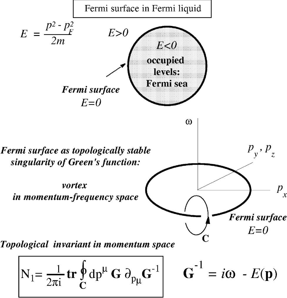
FIG. 1.: Fermi surface as a topological object in momentum space. Top: In the Fermi gas the Fermi surface bounds the solid Fermi sphere of the occupied negative energy states. Bottom: Fermi surface survives even if the interaction between the particles is introduced. The reason for that is that the Fermi surface is the topologically stable object: it is the vortex in the 4D momentum-frequency space $(\omega,{\bf p}$.

In isotropic superconductor and in superfluid ³He-B the energy of quasipartilce is nowhere zero (Fig.2), the gap $\Delta_{0}$ in the spectrum appears as an additional “fundamental constant”

$$E^{2}({\bf p})\rightarrow\Delta_{0}^{2}+v_{F}^{2}\left(|{\bf p}|-p_{F}\right)^{2}~{},~{}~{}{\rm class~{}~{}~{}(ii)}~{}~{}.$$ (55)

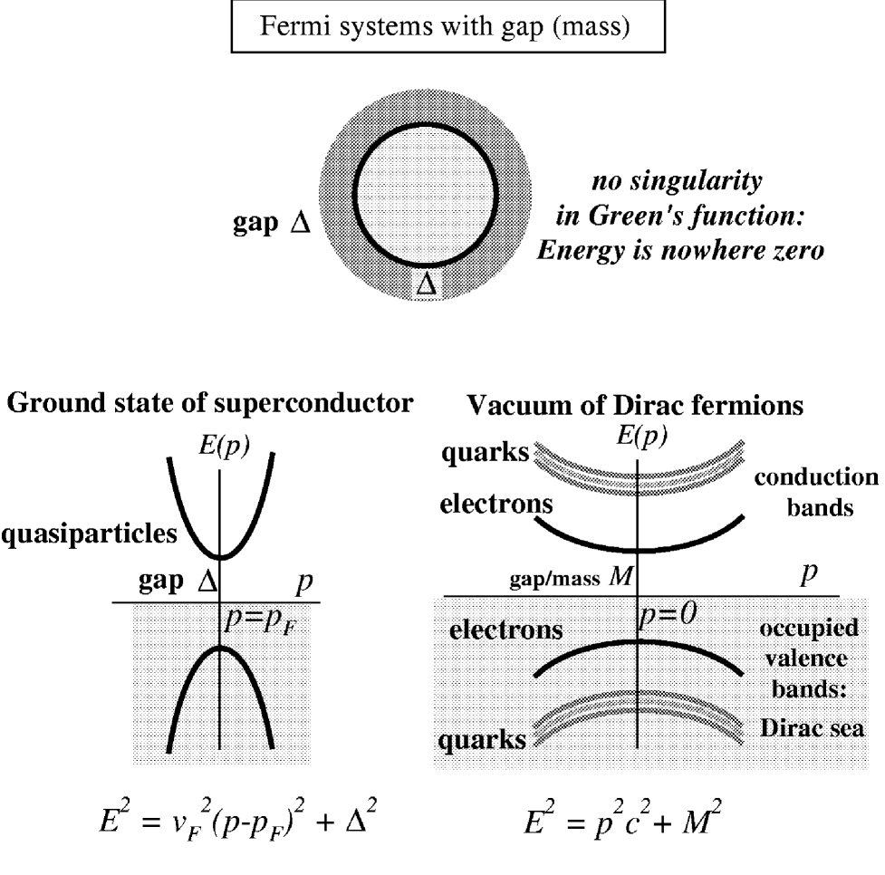
FIG. 2.: Fermi systems with gap or mass. Top: The gap which appears on the Fermi surface in conventional superconductors and in ³He-B. Bottom left: Quasiparticle spectrum in conventional superconductors and ³He-B. Bottom right: The spectrum of Dirac particles and quasiparticle spectrum in semiconductors.

In ³He-A the gap $\Delta({\bf p})$ depends on the direction of the momentum ${\bf p}$: $\Delta^{2}({\bf p})=\Delta_{0}^{2}({\bf p}\times{\hat{\bf l}})^{2}/p_{F}^{2}$. It becomes zero in two opposite directions called the gap nodes – along and opposite to the unit vector ${\hat{\bf l}}$. As a result the quasiparticle energy is zero at two isolated points ${\bf p}=\pm p_{F}{\hat{\bf l}}$ in 3D momentum space (Fig. 3). Close to the gap node at ${\bf p}={\bf p}_{0}$ the spectrum has a form

$$E^{2}({\bf p})\rightarrow g^{ik}(p_{i}-p_{0i})(p_{i}-p_{0k})~{},~{}~{}{\rm class~{}~{}~{}(iii)}~{}~{}.$$ (56)

These three spectra represent three topologically distinct universality classes of the fermionic vacuum in 3+1 dimension: (i) Systems with Fermi surface (Fig. 1); (ii) Systems with gap or mass (Fig. 2); and (iii) Systems with Fermi points (Fig. 3). Systems with the Fermi lines in the spectrum are topologically unstable and by small perturbations can be transformed to one of the three classes. The same topological classification is applicable to the fermionic vacua in high energy physics. The vacuum of Dirac fermions, with the excitation spectrum $E^{2}({\bf p})\rightarrow M^{2}+c^{2}|{\bf p}|^{2}$, belongs to the class (ii). The vacuum of the Weyl fermions in the Standard Model, with the excitation spectrum $E^{2}({\bf p})\rightarrow c^{2}|{\bf p}|^{2}$, belongs to the class (iii). As we shall see below, the latter class is very special, since in this class the relativistic quantum field theory with chiral fermions emerges in the low energy corner, while the collective fields form the gauge fields and gravity.

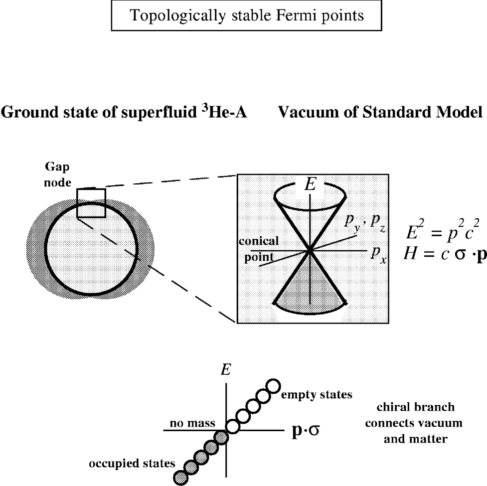
FIG. 3.: Top: Gap node in superfluid ³He-A is the conical point in the energy-momentum space. Bottom: The spectrum of the right-handed chiral particle particle: its spin ${\bf\sigma}$ is oriented along the momentum ${\bf p}$. Quasiparticles in the vicinity of the nodes in ³He-A and elementary particles in the Standard Model above the electroweak transition are chiral fermions.

³He liquids present examples of all 3 classes. The normal ³He liquid at $T>T_{c}$ and also the “high energy physics” of superfluid ³He phases (with energy $E\gg\Delta_{0}$) are representative of the class (i). Below the superfluid transition temperature $T_{c}$ one has either an isotropic superfluid ³He-B of the class (ii) or superfluid ³He-A, which belongs to the class (iii), where the relativistic quantum field theory with chiral fermions gradually arises at low temperature. The great advantage of superfuid ³He-A is that it can be described by the BCS theory, which incorporates all the hierarchy of the energy scales: The “transPlanckian” scale of energies $E\gg\Delta_{0}$ which in the range $v_{F}p_{F}\gg E\gg\Delta_{0}$ is described by the effective theory of universality class (i); the “Planck” scale physics at $E\sim\Delta_{0}$; and the low-energy physics of energies $E\ll\Delta_{0}^{2}/v_{F}p_{F}$ which is described by the effective relativistic theory of universality class (iii). Let us start with the universality class (i).

A Fermi surface as topological object

The Fermi surface (Fig.1) naturally appears in the noninteracting Fermi gas, where the energy spectrum of fermions is

$$E(p)={p^{2}\over 2m}-\mu~{},$$ (57)

and $\mu>0$ is as before the chemical potential. The Fermi surface bounds the volume in the momentum space where the energy is negative, $E(p)<0$, and where the particle states are all occupied at $T=0$. In this isotropic model the Fermi surface is a sphere of radius $p_{F}=\sqrt{2m\mu}$. Close to the Fermi surface the energy spectrum is $E(p)\approx v_{F}(p-p_{F})$, where $v_{F}=\partial_{p}E|_{p=p_{F}}$ is the Fermi velocity.

It is important that the Fermi surface survives even if interactions between particles are introduced. Such stability of the Fermi surface comes from the topological property of the Feynman quantum mechanical propagator – the one-particle Green’s function

$${\cal G}=(z-{\cal H})^{-1}~{}.$$ (58)

Let us write the propagator for a given momentum ${\bf p}$ and for the imaginary frequency, $z=ip_{0}$. The imaginary frequency is introduced to avoid the conventional singularity of the propagator “on the mass shell”, i.e. at $z=E(p)$. For noninteracting particles the propagator has the form

$$G={1\over ip_{0}-v_{F}(p-p_{F})}~{}.$$ (59)

Obviously there is still a singularity: On the 2D hypersurface $(p_{0}=0,p=p_{F})$ in the 4-dimensional space $(p_{0},{\bf p})$ the propagator is not well defined. This singularity is stable, i.e. it cannot be eliminated by small perturbations. The reason is that the phase $\Phi$ of the Green’s function $G=|G|e^{i\Phi}$ changes by $2\pi$ around the path $C$ embracing this 2D hypersurface in the 4D-space (see the bottom of Fig.1, where one dimension is skipped, so that the Fermi surface is presented as a closed line in 3D space). The phase winding number $N_{1}=1$ cannot change continuously, that is why it is robust towards any perturbation. Thus the singularity of the Green’s function on the 2D-surface in the momentum space is preserved, even when interactions between particles are introduced.

Exactly the same topological conservation of the winding number leads to the stability of the quantized vortex in superfluids and superconductors, the only difference being that, in the case of vortices, the phase winding occurs in the real space, instead of the momentum space. The complex order parameter $\Psi=|\Psi|e^{i\Phi}$ changes by $2\pi n_{1}$ around the path embracing the vortex line in 3D space or vortex sheet in 3+1 space-time. The connection between the space-time topology and the energy-momentum space topology is, in fact, even deeper (see e.g. Ref.[25]). If the order parameter depends on space-time, the propagator in semiclassical aproximation depends both on 4-momentum and on space-time coordinates $G(p_{0},{\bf p},t,{\bf r})$. The topology in the 4+4 dimensional space describes: the momentum space topology of the homogeneous system; topological defects of the order parameter in space-time; topology of the energy spectrum within the topological defects [26]; and quantization of physical parameters (see Section IV D).

In the more complicated cases, when the Green’s function is the matrix with spin and band indices, the phase of the Green’s function becomes meaningless. In this case one should use a general analytic expression for the integer momentum-space topological invariant which is responsible for the stability of the Fermi surface:

$$N_{1}={\bf Tr}~{}\oint_{C}{dl\over 2\pi i}{\cal G}(p_{0},p)\partial_{l}{\cal G}^{-1}(p_{0},p)~{}.$$ (60)

Here the integral is taken over an arbitrary contour $C$ in the momentum space $({\bf p},p_{0})$, which encloses the Fermi hypersurface (Fig. 1 bottom); and ${\bf Tr}$ is the trace over the spin and band indices.

1 Landau Fermi liquid

The topological class of systems with Fermi surface is rather broad. In particular it contains conventional Landau Fermi-liquids, in which the propagator preserves the pole. Close to the pole the propagator is

$$G={Z\over ip_{0}-v_{F}(p-p_{F})}~{}.$$ (61)

Evidently the residue $Z\neq 1$ does not change the topological invariant for the propagator, Eq.(60), which remains $N_{1}=1$. This is essential for the Landau theory of an interacting Fermi liquid; it confirms the assumption that there is one to one correspondence between the low energy quasiparticles in Fermi liquids and particles in a Fermi gas. It is also important for the consideration of the bosonic collective modes of the Landau Fermi-liquid. The interaction between the fermions cannot not change the topology of the fermionic spectrum, but it produces the effective field acting on a given particle by the other moving particles. This effective field cannot destroy the Fermi surface owing to its topological stability, but it can locally shift the position of the Fermi surface. Therefore a collective motion of the particles is seen by an individual quasiparticle as dynamical modes of the Fermi surface (Fig. 4. These bosonic modes are known as the different harmonics of the zero sound [11].

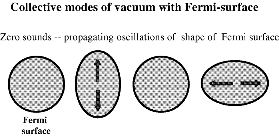
FIG. 4.: Bosonic collective modes in the fermionic vacuum of the Fermi-surface universality class. Collective motion of particles comprising the vacuum is seen by an individual quasiparticle as dynamical modes of the Fermi surface. Here the propagating elliptical deformations of the Fermi surface are drawn.

Note that the Fermi hypersurface exists for any spatial dimension. In the 2+1 dimension the Fermi hypersurface is a line in 2D momentum space, which cooresponds to the vortex loop in the 3D frequency-momentum space in Fig. 1.

Topological stability also means that any adiabatic change of the system will leave the system within the same class. Such adiabatic perturbation can include the change of the interaction strength between the particles, deformation of the Fermi surface, etc. Under adiabatic perturbation no spectral flow across the Fermi surface occurs (of course, if the deformation is slow enough), so the state without excitations transforms to the other state, in which excitations are also absent, i.e. the vacuum transforms to the vacuum. The absence of the spectral flow leads in particular to the Luttinger’s theorem which states that the volume of the Fermi surface is invariant under adiabatic deformations, if the number of particles is kept constant [27]. Since the isotropic Fermi liquid can be obtained from the Fermi gas by adiabatical switching on the interaction between the particles, the relation between the particle density and the Fermi momentum remains the same as in the Fermi gas,

$$n={p_{F}^{3}\over 3\pi^{2}\hbar^{3}}~{}.$$ (62)

Topological approach to Luttinger’s theorem has been recently discussed in [28]. The processes related to the spectral flow of quasiparticle energy levels will be considered in Sections VII and IX in connection with the phenomenon of axial anomaly.

2 Non-Landau Fermi liquids

In the 1+1 dimension, the Green’s function looses its pole but nevertheless the Fermi surface is still there [29, 30]. Though the Landau Fermi liquid transforms to another states, this occurs within the same topological class with given $N_{1}$. An example is provided by the Luttinger liquid. Close to the Fermi surface the Green’s function for the Luttinger liquid can be approximated as (see [31, 29, 32])

$$G(z,p)\sim$$ (63)

$$(ip_{0}-v_{1}\tilde{p})^{g-1\over 2}(ip_{0}+v_{1}\tilde{p})^{g\over 2}(ip_{0}-v_{2}\tilde{p})^{g-1\over 2}(ip_{0}+v_{2}\tilde{p})^{g\over 2}$$ (64)

where $v_{1}$ and $v_{2}$ correspond to Fermi velocities of spinons and holons and $\tilde{p}=p-p_{F}$. The above equation is not exact but reproduces the momentum space topology of the Green’s function in Luttinger Fermi liquid. If $g\neq 0$ and $v_{1}\neq v_{2}$, the singularity in the $(\tilde{p},z=ip_{0})$ momentum space occurs on the Fermi surface, i.e. at $(p_{0}=0,~{}\tilde{p}=0)$. The momentum space topological invariant in Eq.(60) remains the same $N_{1}=1$, as for the conventional Landau Fermi-liquid. The difference from Landau Fermi liquid occurs only at real frequency $z$: The quasiparticle pole is absent and one has the branch cut singularities instead of the mass shell, so that the quasiparticles are not well defined. The population of the particles has no jump on the Fermi surface, but has a power-law singularity in the derivative [30].

Another example of the non-Landau Fermi liquid is the Fermi liquid with exponential behavior of the residue [33]. It also has the Fermi surface with the same topological invariant, but the singularity at the Fermi surface is exponentially weak.

B Fully gapped systems: “Dirac particles” in superconductors and in superfluid ³He-B

Although the systems we have discussed in Sec.IV A contain fermionic and bosonic quantum fields, this is not the relativistic quantum field theory which we need for the simulation of quantum vacuum: There is no Lorentz invariance and the oscillations of the Fermi surface do not resemble the gauge field even remotely. The situation is somewhat better for superfluids and superconductors with fully gapped spectra. For example, the Nambu-Jona-Lasinio model in particle physics provides a parallel with conventional superconductors [34]; the symmetry breaking scheme in superfluid ³He-B was useful for analysis of the color superconductivity in quark matter [35].

In ³He-B the Hamiltonian of free Bogoliubov quasiparticles is the $4\times 4$ matrix (see Eq.(91) below):

$${\cal H}=\left(\matrix{M({\bf p})&c{\bf\sigma}\cdot{\bf p}\cr c{\bf\sigma}\cdot{\bf p}&-M({\bf p})\cr}\right)={\check{\tau}}_{3}M({\bf p})+c{\check{\tau}}_{1}{\bf\sigma}\cdot{\bf p}~{},$$ (65)

$$M({\bf p})={p^{2}\over 2m}-\mu\approx v_{F}(p-p_{F})~{},~{}c={\Delta_{0}\over p_{F}}~{}~{}~{},~{}~{}~{}{\cal H}^{2}=E^{2}\approx M^{2}({\bf p})+\Delta_{0}^{2}~{},~{}$$ (66)

where the Pauli $2\times 2$ matrices ${\bf\sigma}$ describe the conventional spin of fermions and $2\times 2$ matrices $\check{\bf\tau}$ describe the Bogoliubov-Nambu isospin in the particle-hole space (see Sec.V A 2). The Bogoliubov-Nambu Hamiltonian becomes “relativistic” in the limit $mc^{2}\gg\mu$, where it asymptotically approaches the Dirac Hamiltonian for relativistic particles of mass $\mu$. However in a real ³He-B one has an opposite limit $mc^{2}\ll\mu$ and the energy spectrum is far from being “relativistic”. Nevertheless ³He-B also serves as a model system for simulations of phenomena in particle physics and cosmology. In particular, vortex nucleation in nonequilibrium phase transition has been observed [36] as experimental verification of the Kibble mechanism describing formation of cosmic strings in expanding Universe [37]; the global vortices in ³He-B were also used for experimental simulation of the production of baryons by cosmic strings mediated by spectral flow [38] (see Sec.IX).

C Systems with Fermi points

1 Chiral particles and Fermi point

In particle physics the energy spectrum $E({\bf p})=cp$ is characteristic of the massless chiral fermion, lepton or quark, in the Standard Model with $c$ being the speed of light. As distinct from the case of Fermi surface, where the energy of quasiparticle is zero at the surface in 3D momentum space, the energy of a chiral particle is zero at the point ${\bf p}=0$. We call such point the Fermi point. The Hamiltonian for the massless spin-1/2 particle is a $2\times 2$ matrix

$${\cal H}=\pm c{\bf\sigma}\cdot{\bf p}$$ (67)

which is expressed in terms of the Pauli spin matrices ${\bf\sigma}$. The sign $+$ is for a right-handed particle and $-$ for a left-handed one: the spin of the particle is oriented along or opposite to its momentum, respectively.

2 Topological invariant for Fermi point

Even if the Lorentz symmetry is violated far from the Fermi point, the Fermi point will survive. The stability of the Fermi point is prescribed by the mapping of the surface $S_{2}$ surrounding the degeneracy point in 3D-momentum space into the complex projective space $CP^{N-1}$ of the eigenfunction $\omega({\bf p})$ of $N\times N$ Hamiltonian describing the fermion with $N$ components [39] ($N=2$ for one Weyl spinor). The topological invariant can be written analytically in terms of the Green’s function ${\cal G}=(ip_{0}-{\cal H})^{-1}$ determined on the imaginary frequency axis, $z=ip_{0}$ [40] (Fig.5). One can see that this propagator has a singularity at the point in the 4D momentum-frequency space: $(p_{0}=0,{\bf p}=0)$. The invariant is represented as the integral around the 3-dimensional surface $\sigma$ embracing such singular point

$$N_{3}={1\over{24\pi^{2}}}e_{\mu\nu\lambda\gamma}~{}{\bf tr}\int_{\sigma}~{}dS^{\gamma}~{}{\cal G}\partial_{p_{\mu}}{\cal G}^{-1}{\cal G}\partial_{p_{\nu}}{\cal G}^{-1}{\cal G}\partial_{p_{\lambda}}{\cal G}^{-1}~{}.$$ (68)

Here ${\cal G}$ is an arbitrary matrix function of ${\bf p}$ and $p_{0}$, which is continuous and differentiable outside the singular point. One can check that under continuous variation of the matrix function the integrand changes by the full derivative. That is why the integral over the closed 3-surface does not change, i.e. $N_{3}$ is invariant under continuous deformations of the Green’s function and also of the closed 3-surface. The possible values of the invariant can be easily found: if one chooses the matrix function which changes in $U(2)$ space one obtains the integer values of $N_{3}$. They describe the mapping of the $S^{3}$ sphere surrounding the degeneracy point in 4-space of the energy-momentum $(p_{0},{\bf p})$ into the $SU(2)=S^{3}$ space. The same integer values $N_{3}$ are preserved for any Green’s function matrix, if it is well determined, i.e. if ${\rm det}~{}G^{-1}\neq 0$. The index $N_{3}$ thus represent topologically different Fermi points – the singular points in 4D momentum-frequency space.

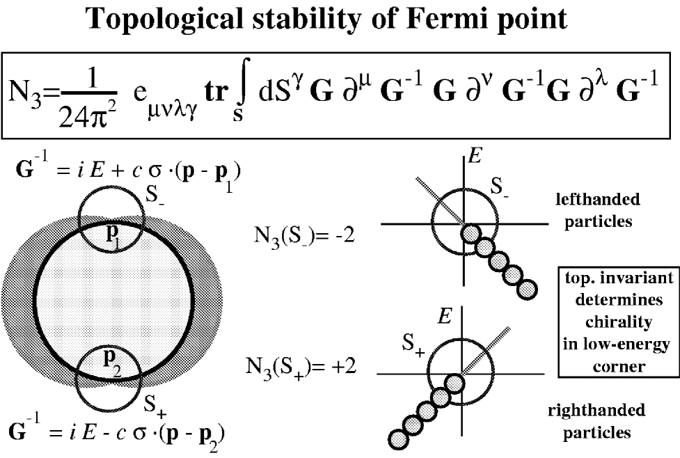
FIG. 5.: The Green’s function for fermions in ³He-A and in the Standard Model have point singularity in the 4D momentum-frequency space, which is described by the integer-valued topological invariant $N_{3}$. The Fermi points in ³He-A at ${\bf p}=\pm p_{F}{\hat{\bf l}}$ have $N_{3}=\mp 2$. The Fermi point at ${\bf p}$ for the chiral relativistic particle in Eq. (67) has $N_{3}=C_{a}$, where $C_{a}=\pm 1$ is the chirality. The chirality, however, appears only in the low energy corner together with the Lorentz invariance. Thus the topological index $N_{3}$ is the generalization of the chirality to the Lorentz noninvariant case.

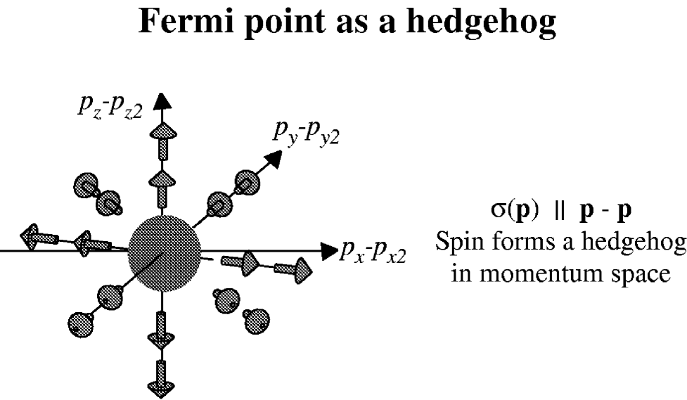
FIG. 6.: Illustration of the meaning of the topological invariant for the simplest case: Fermi point as a hedgehog in 3D momentum space. For each momentum ${\bf p}$ we draw the direction of the quasiparticle spin, or its equivalent in ³He-A – the Bogoliubov spin. Topological invariant for the hedgehog is the mapping $S^{\rightarrow}S^{2}$ with integer index $N_{3}$ which is $N_{3}=+1$ for the drawn case of right-handed particle. The topological invariant $N_{3}$ is robust to any deformation of the spin field ${\bf\sigma}({\bf p})$: one cannot comb the hedgehog smooth.

3 Topological invariant as the generalization of chirality.

For the chiral fermions in Eq.(67) this invariant has values $N_{3}=C_{a}$, where $C_{a}=\pm 1$ is the chirality of the fermion. For this case the meaning of this topological invariant can be easily visualized (Fig. 6). Let us consider the behavior of the particle spin ${\bf s}({\bf p})$ as a function the particle momentum ${\bf p}$ in the 3D-space ${\bf p}=(p_{x},p_{y}.p_{z})$. For the right-handed particle, whose spin is parallel to the momentum, one has ${\bf s}({\bf p})={\bf p}/2p$, while for left-handed ones ${\bf s}({\bf p})=-{\bf p}/2p$. In both cases the spin distribution in the momentum space looks like a hedgehog, whose spines are represented by spins. Spines point outward for the right-handed particle producing the mapping of the sphere $S^{2}$ in 3D momentum space onto the sphere $S^{2}$ of the spins with the index $N_{3}=+1$. For the left-handed particle the spines of the hadgehog look inward and one has the mapping with $N_{3}=-1$. In the 3D-space the hedgehog is topologically stable.

What is important here that the Eq.(68), being the topological invariant, does not change under any (but not very large) perturbations. This means that even if the interaction between the particles is introduced and the Green’s functions changes drastically, the result remains the same: $N_{3}=1$ for the righthanded particle and $N_{3}=-1$ for the lefthanded one. The singularity of the Green’s function remains, which means that the quasiparticle spectrum remain gapless: fermions are massless even in the presence of interaction.

Above we considered the relativistic fermions. However, the topological invariant is robust to any deformation, including those which violate the Lorentz invariance. This means that the topological description is far more general than the description in terms of chirality, which is valid only when the Lorentz symmetry is obeyed. In paticular, the notion of the Fermi point can be extended to the nonrelativistic condensed matter, such as superfluid ³He-A (Fig. 5), while the chirality of quasiparticles is not determined in the nonrelativistic system. This means that the charge $N_{3}$ is the topological generalization of chirality.

From the topological point of view the Standard Model and the Lorentz noninvariant ground state of ³He-A belong to the same universality class of systems with Fermi points, though the underlying “microscopic” physics can be essentially different.

4 Relativistic massless chiral fermions emerging near Fermi point.

The most remarkable property of systems with the Fermi point is that the relativistic invariance always emerges at low energy. Close to the Fermi point $p_{\mu}^{(0)}$ in the 3+1 momentum-energy space one can expand the propagator in terms of the deviations from this Fermi point, $p_{\mu}-p_{\mu}^{(0)}$. If the Fermi point is not degenerate, i.e. $N_{3}=\pm 1$, then close to the Fermi point only the linear deviations survive. As a result the general form of the inverse propagator is

$${\cal G}^{-1}=\sigma^{a}e^{\mu}_{a}(p_{\mu}-p_{\mu}^{(0)})~{}.$$ (69)

Here we returned back from the imaginary frequency axis to the real energy, so that $z=E=-p_{0}$ instead of $z=ip_{0}$; and $\sigma^{a}=(1,{\bf\sigma})$. The quasiparticle spectrum $E({\bf p})$ is given by the poles of the propagator, and thus by equation

$$g^{\mu\nu}(p_{\mu}-p_{\mu}^{(0)})(p_{\nu}-p_{\nu}^{(0)})=0~{},~{}g^{\mu\nu}=\eta^{ab}e^{\mu}_{a}e^{\nu}_{b}~{},$$ (70)

where $\eta^{ab}=diag(-1,1,1,1)$. Thus in the vicinity of the Fermi point the massless quasiparticles are always described by the Lorentzian metric $g^{\mu\nu}$, even if the underlying Fermi system is not Lorentz invariant; superfluid ³He-A is an example (see next Section). On this example we shall also see that the quantities $g^{\mu\nu}$ and $p_{\mu}^{(0)}$ are dynamical variables, related to the collective modes of ³He-A, and they play the part of the effective gravity and gauge fields correspondingly (Fig. 7).

In conclusion, from the condensed matter point of view, the classical (and quantum) gravity is not a fundamental interaction. Matter (chiral particles and gauge fields) and gravity (vierbein or metric field) inevitably appear together in the low energy corner as collective fermionic and bosonic zero modes of the underlying system, if the system belongs to the universality class with Fermi points.

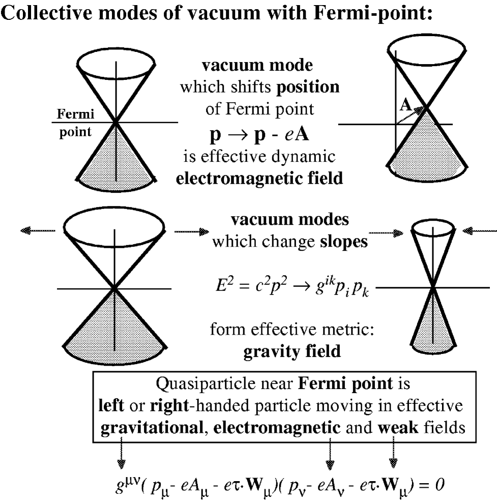
FIG. 7.: Bosonic collective modes of the fermionic vacuum which belongs to the Fermi-point universality class. The slow (low-energy) vacuum motion cannot destroy the topologically stable Fermi point, it can only shift the point and/or change its slopes. The shift corresponds to the change of the gauge field ${\bf A}$, while the slopes (“speeds of light”) form the metric tensor $g^{ik}$. are oscillating Collective motion of particles comprising the vacuum is thus seen by an individual quasiparticle as gauge and gravity fields. Thus the chiral fermions, gauge fields and gravity appear in low-energy corner together with physical laws: Lorentz, gauge, conformal invariance and general covariance.

D Gapped systems with nontrivial topology in 2+1 dimensions

Even for the fully gapped systems there can exist the momentum-space topological invariants, which characterize the vacuum states. Typically this occurs in 2+1 systems, e.g. in the 2D electron system exhibiting quantum Hall effect [43]; in thin film of ³He-A (see [41] and Sec.9 of Ref.[40]); in the 2D superconductors with broken time reversal symmetry [42]; in the 2+1 world of fermions living within the domain walls. The quantum (Lifshitz) transition between the states with different topological invariants occurs through the intermediate gapless regime [40].

The ground states, vacua, in 2D systems or in quasi-2D thin films are characterized by invariants of the type

$$N_{3}={1\over{24\pi^{2}}}e_{\mu\nu\lambda}~{}{\bf tr}\int d^{2}pdp_{0}~{}{\cal G}\partial_{p_{\mu}}{\cal G}^{-1}{\cal G}\partial_{p_{\nu}}{\cal G}^{-1}{\cal G}\partial_{p_{\lambda}}{\cal G}^{-1}~{},$$ (71)

The integral now is over the whole 3D momentum-energy space $p_{\mu}=(p_{0},p_{x},p_{y})$, or if the crystalline system is considered the integration over $p_{x},p_{y}$ is bounded by Brillouin zone. The integrand is determined everywhere in this space since the system is fully gapped and thus the Green’s function is nowhere singular. In thin films, in addition to spin indices, the Green’s function matrix ${\cal G}$ contains the indices of the transverse levels, which come from quantization of motion along the normal to the film [40]. Fermions on different transverse levels represent different families of fermions with the same properties. This would correspond to generations of fermions in the Standard Model, if our 3D world is situated within the soliton wall in 4D space.

The topological invariants of the type in Eq.(71) determine the anomalous properties of the film. In particular, they are responsible for quantization of physical parameters, such as Hall conductivity [43] and spin Hall conductivity [41, 44, 45]. The Eq.(71) leads to quantization of the $\theta$-factor [41]

$$\theta={\pi\over 2}~{}N_{3}~{},$$ (72)

in front of the Chern-Simons term

$$S_{\theta}={\hbar\theta\over{32\pi^{2}}}\int d^{2}x\hskip 2.84526ptdt\hskip 2.84526pte^{\mu\nu\lambda}A_{\mu}F_{\nu\lambda}~{},~{}F_{\nu\lambda}=\partial_{\nu}A_{\lambda}-\partial_{\lambda}A_{\nu}=\hat{\bf d}\cdot\left(\partial_{\nu}\hat{\bf d}\times\partial_{\lambda}\hat{\bf d}\right),$$ (73)

where $\hat{\bf d}$ is unit vector characterizing the fermionic spectrum. The $\theta$-factor determines the quantum statistics of the skyrmions. They are fermions or bosons depending on the thickness of the film and their statistics abruptly changes when the film grows [40]. For more general 2+1 condensed matter systems with different types of momentum-space invariants, see [46].

The action in Eq.(73) represents the product of two topological invariants: $N_{3}$ in momentum space and Hopf invariant in 2+1 coordinate space-time. This is an example of topological term in action characterized by combined momentum-space/real-space topology.

V Fermi points: ³He-A vs Standard Model

The reason why all the attributes of the relativistic quantum field theory arise from nothing in ³He-A is that both systems, the Standard Model and ³He-A, have the same topology in momentum space. The energy spectrum of fermions in ³He-A also contains point zeroes, the gap nodes, which are described by the same topological invariant in the momentum space in Eq.(68) (see Fig. 5). For one isolated Fermi point the nonzero topological invariant gives singularity in the Green’s function and thus the gapless spectrum, which for the relativistic system means the absence of the fermion mass.

It appears, however, that in both systems the total topological charge of all the Fermi points in the momentum space is zero. In ³He-A one has $\sum_{a}N_{3a}=2-2=0$. Nevertheless, the separation of zeroes in momentum space prohibits masses for fermions. The mass can appear when the Fermi points merge. But even in this case the absence of the fermionic mass can be provided by the symmetry of the system. This happens in the so called planar phase of ³He [13] and also in the Standard Model, where the for each Fermi point one has $\sum_{a}N_{3a}=\sum_{a}C_{a}=0$, but the discrete symmetry in the planar phase of ³He-A and the electroweak symmetry in the Standard Model prohibit masses for fermions. Fermions become massive when this symmetry is broken. This will be discussed in more detail in Sec.V B (see also ref. [47]).

A Superfluid ³He-A

1 Fermi liquid level.

In ³He-A, the number of Fermi points and thus the number of Fermionic species is essentially smaller than in the Standard Model of strong ane electroweak interactions. In place of the various quarks and leptons, there are only four species occurring as left and right “weak” doublets. One way to write these might be [48]

$$\chi_{L}=\pmatrix{\nu\cr e\cr}_{L}\ ,\chi_{R}=\pmatrix{\nu\cr e\cr}_{R}\ .$$ (74)

In this section we discuss how this is obtained.

The pair-correlated systems (superconductors and ³He superfluids) in their unbroken symmetry state above $T_{c}$ belong to the class of Fermi systems with Fermi surface. In terms of the field operator $\psi_{\alpha}$ for ³He atoms the action is

$$S=\int dt~{}d^{3}x~{}\left[\psi^{\dagger}_{\alpha}\left(i\partial_{t}-{{{\bf p}^{2}}\over{2m}}+\mu\right)\psi_{\alpha}\right]~{}+~{}S_{int}\ ,$$ (75)

where $S_{int}$ includes the time-independent interaction of two atoms (the quartic term), $m$ is the mass of ³He atom, ${\bf p}=-i\nabla$ is the momentum operator and $\mu$ is the chemical potential. In general this system is described by the large number of fermionic degrees of freedom. However, in the low-temperature limit, the number of degrees of freedom is effectively reduced and the system is well described as a system of noninteracting quasiparticles (dressed particles). Since the Fermi liquid belongs to the same universality class as the weakly interacting Fermi gas, at low energy one can map it to the Fermi gas degrees of freedom. This is the essence of the Landau theory of Fermi liquids. The particle-particle interaction renormalizes the effective mass of quasiparticle: $m\rightarrow m^{*}$. The residual interaction is reduced at low $T$ because of the small number of thermal quasiparticles above the Fermi-surface and can be neglected. Thus the effective action for quasiparticles becomes

$$S=\int dt~{}d^{3}x~{}\psi^{\dagger}_{\alpha}[i\partial_{t}-M({\bf p})]\psi_{\alpha}~{}~{},$$ (76)

where $M({\bf p})$ is the quasiparticle energy spectrum. In a Fermi-liquid this description is valid in the so called degeneracy limit, when the temperature $T$ is much smaller than the effective Fermi temperature, $\Theta\sim\hbar^{2}/(ma^{2})$, which plays the part of the Planck energy in the Fermi liquid. Here $a$ is again the interparticle distance in the liquid. Further for simplicity we use the following Ansatz for the quasiparticle energy in Fermi liquid

$$M({\bf p})={p^{2}-p_{F}^{2}\over 2m^{*}}\approx v_{F}(p-p_{F})$$ (77)

where $m^{*}$ is the renormalized mass of the quasiparticle, and the Fermi velocity is now; the last expression is the most general form of the low-energy spectrum of excitations in the isotropic Landau Fermi liquids in the vicinity of the Fermi surface.

2 BCS level.

Below the superfluid/superconducting transition temperature $T_{c}$, new collective degrees of freedom appear, which are the order parameter fields, corresponding to the Higgs field in particle physics. In superconductors the order parameter is the vacuum expectation value of the product of two annihilation operators (Cooper pair wave function)

$$\Delta\propto<{\rm vac}|\psi\psi|{\rm vac}>~{}~{}.$$ (78)

The order parameter $\Delta$ is a $2\times 2$ matrix in conventional spin space. It breaks the global $U(1)_{N}$ symmetry $\psi_{\mu}\rightarrow e^{i\alpha}{\bf\psi}_{\mu}$, which is responsible for the conservation of the particle number $N$ of ³He atoms, since under $U(1)_{N}$ the order parameter transforms as $\Delta(x,y)\rightarrow e^{2i\alpha}\Delta(x,y)$. If $\Delta$ has nontrivial spin and orbital structure, it also breaks the $SO(3)_{L}$ and $SO(3)_{S}$ symmetries under rotations in orbital and spin spaces correspondingly.

The interaction of the fermionic degrees of freedom with the order parameter can be obtained in BCS model using the Hubbard-Stratonovich procedure. The essence of this procedure, which can be easily visualized if one omits all the coordinate dependence and spin indices, is the decomposition of pair interaction $S_{int}=\int g\psi^{\dagger}\psi^{\dagger}\psi\psi$, where $g$ is the generalized interaction potential. The formal way is to introduce the constant Gaussian term in the path integral $\int d\Delta~{}d\Delta^{*}\exp(i\Delta~{}\Delta^{*}/g)$ and shift the argument $\Delta\rightarrow\Delta-\psi\psi$. In this way the quartic term in action is cancelled and one has the BCS action with only quadratic forms:

$$S=\int dt~{}d^{3}x~{}\psi^{\dagger}_{\alpha}\left[i\partial_{t}-M({\bf p})\right]\psi_{\alpha}$$ (79)

$$+\int dt~{}d^{3}x~{}d^{3}y~{}[\psi^{\dagger}_{\alpha}(x){\bf\psi}^{\dagger}_{\beta}(y)\Delta_{\alpha\beta}(x,y)+\Delta_{\alpha\beta}^{\star}(x,y)\psi_{\beta}(y)\psi_{\alpha}(x)]$$ (80)

$$-\int{|\Delta|^{2}\over g}~{}.$$ (81)

The last term is the symbolic form of the quadratic form of the order parameter.

The interaction of fermions with the bosonic order parameter field in Eq.(80) allows transitions between states differing by two atoms, $N$ and $N\pm 2$. The order parameter $\Delta$ serves as the matrix element of such transition. This means that the particle number $N$ is not conserved in the broken symmetry state and the single-fermion elementary excitation of this broken symmetry vacuum represents the mixture of the $N=1$ (particle) and $N=-1$ (hole) states.

In electroweak theory the interactions corresponding to those in Eq.(80) are the Yukawa coupling which appear in the broken symmetry state between the left-handed $SU(2)_{L}$ doublets and the right-handed fermion singlets. An example of such an interaction is the term:

$$G_{d}({\bar{u}},{\bar{d}})_{L}\Phi d_{R}$$ (82)

in the electroweak Lagrangian. When $\Phi$ acquires a vacuum expectation value during the electroweak phase transition, this gives rise to the nonconservation of the isospin and hypercharge in the same manner as the charge $N$ is not conserved in the broken symmetry action Eq.(80). Such hybridization of left and right particles leads to the lepton and quark masses. Similarly, in superfluids and superconductors these terms give rise to the gap on the Fermi surface.

However, the more close link to the BCS has the color superconductivity in quark matter [35], where the order parameter is the matrix element between the states differing by two quarks. Among the different phases of the color superconductivity there is a representative of the Fermi point universality class, the phase where the gap hass point node like in ³He-A [49].

For the $s$-wave spin-singlet pairing in superconductors and the $p$-wave spin-triplet pairing in superfluid ³He the matrix element has the following general form:

$$\Delta_{s-{\rm wave}}({\bf r},{\bf p})=i\sigma^{(2)}\Psi({\bf r})~{}~{},$$ (83)

$$\Delta_{p-{\rm wave}}({\bf r},{\bf p})=i\sigma^{(\mu)}\sigma^{(2)}A_{\mu\,i}({\bf r})p_{i}~{}~{}.$$ (84)

Here ${\bf\sigma}$ are the Pauli matrices in spin space, ${\bf r}=({\bf x}+{\bf y})/2$ is the center of mass coordinate of the Cooper pair, while the momentum ${\bf p}$ describes the relative motion of the two fermions within the Cooper pair: it is the Fourier transform of the coordinates $({\bf x}-{\bf y})$. The complex scalar function $\Psi({\bf r})$ and $3\times 3$ matrix $A_{\mu\,i}({\bf r})$ are the order parameters for $s$- and $p$-wave pairing respectively, which are space independent in global equilibrium.

Two superfluid states with $p$-wave pairing are realized in ³He. The state which belongs to the Fermi point universality class is the ³He-A phase. In ³He-A the matrix order parameter is factorized into the product of the spin part described by the real unit vector $\hat{\bf d}$ and the orbital part described by the complex vector $\hat{\bf e}_{1}+i\hat{\bf e}_{2}$

$$A_{\mu\,i}=\Delta_{0}\hat{d}_{\mu}\left(\hat{e}_{1i}+i\hat{e}_{2i}\right)~{}~{},~{}~{}\hat{\bf e}_{1}\cdot\hat{\bf e}_{1}=\hat{\bf e}_{2}\cdot\hat{\bf e}_{2}=1~{}~{},~{}~{}\hat{\bf e}_{1}\cdot\hat{\bf e}_{2}=0~{}.$$ (85)

The ³He-B belongs to the universality class with gap, its the matrix order parameter is

$$A_{\mu\,i}=\Delta_{0}R_{\mu\,i}e^{i\theta}~{},$$ (86)

where $R_{\mu\,i}$ is the real orthogonal matrix. These two broken symmetry vacua correspond to two different routes of the symmetry breaking: $U(1)_{N}\times SO(3)_{L}\times SO(3)_{S}\rightarrow U(1)_{N-L}\times U(1)_{S}$ for ³He-A and $U(1)_{N}\times SO(3)_{L}\times SO(3)_{S}\rightarrow SO(3)_{S+L}$ for ³He-B.

The easiest way to treat the action in Eq.(79-81), in which the states with 1 particle and -1 particle are hybridized by the order parameter, is to double the number of degrees of freedom introducing the antiparticle (hole) for each particle by introducing the Bogoliubov-Nambu field operator $\chi$. It is the spinor in a new particle-hole space (Nambu space):

$${\bf\chi}=\pmatrix{{\bf u}\cr{\bf v}\cr}=\pmatrix{\Phi\cr i\sigma^{(2)}\Phi^{\dagger}\cr}~{}~{};~{}~{}{\bf\chi}^{\dagger}=({\bf u}^{\dagger}~{},~{}{\bf v}^{\dagger})~{}~{}.$$ (87)

Under $U(1)_{N}$ symmetry operation $\Phi_{\alpha}\rightarrow e^{i\phi}\Phi_{\alpha}$ this spinor transforms as

$${\bf\chi}\rightarrow e^{i\check{\tau}_{3}\phi}{\bf\chi}~{}~{}.$$ (88)

Here $\check{\tau}_{i}$ are Pauli matrices in the Nambu space, such that $\check{\tau}_{3}$ is the particle number operator ${\bf N}$ with eigenvalues $+1$ for the particle component of the quasiparticle and $-1$ for its hole component.

The eigenvalue equation for the quasiparticle spectrum is

$${\cal H}\chi=E\chi~{}~{},$$ (89)

where the Hamiltonian for quasiparticles in $s$-wave superconductors:

$${\cal H}_{s-{\rm wave}}=M({\bf p})\check{\tau}_{3}+\pmatrix{0&\Psi({\bf r})\cr\Psi^{*}({\bf r})&0\cr}~{}~{};$$ (90)

in the B-phase of ³He:

$${\cal H}_{\rm B-phase}=M({\bf p})\check{\tau}_{3}+{{\Delta_{0}}\over{p_{F}}}({\bf\sigma}\cdot{\bf p})\check{\tau}_{1}~{};$$ (91)

and in ³He-A:

$${\cal H}_{\rm A-phase}=M({\bf p})\check{\tau}_{3}+{{\Delta_{0}}\over{p_{F}}}({\bf\sigma}\cdot\hat{\bf d}({\bf r}))(\check{\tau}_{1}\hat{e}_{1}({\bf r})\cdot{\bf p}-\check{\tau}_{2}\hat{e}_{2}({\bf r})\cdot{\bf p})~{}.$$ (92)

It is also instructive to consider the so called planar phase, where:

$${\cal H}_{\rm planar}=M({\bf p})\check{\tau}_{3}+{{\Delta_{0}}\over{p_{F}}}\check{\tau}_{1}((\hat{e}_{1}({\bf r})\cdot{\bf p})\sigma_{x}+(\hat{e}_{2}({\bf r})\cdot{\bf p})\sigma_{y})~{}.$$ (93)

The square of the fermionic energy in these pair-correletaed states is correspondingly

$$E_{s-{\rm wave}}^{2}({\bf p})={\cal H}^{2}=M^{2}({\bf p})+|\Psi|^{2}~{}~{},$$ (94)

$$E_{{\rm B-phase}}^{2}({\bf p})={\cal H}^{2}=M^{2}({\bf p})+{\Delta_{0}^{2}\over p_{F}^{2}}p^{2}\approx\left({p^{2}-p_{F}^{2}\over 2m^{*}}\right)^{2}+\Delta_{0}^{2}~{}~{},$$ (95)

$$E_{\rm A-phase}^{2}({\bf p})=E_{\rm planar}^{2}({\bf p})={\cal H}^{2}=M^{2}({\bf p})+\left({{\Delta_{0}}\over{p_{F}}}\right)^{2}({\bf p}\times{\bf\hat{l}})^{2}~{}~{},~{}~{}{\bf\hat{l}}={\bf\hat{e}}_{1}\times{\bf\hat{e}}_{2}~{}.$$ (96)

Here we took into accont that $\Delta_{0}\ll v_{F}p_{F}$ in ³He. These equations show that fermionic quasiparticles in the $s$-wave superfluids/superconductors and in ³He-B have a gap in the spectrum and thus belong to the unviersality class of Dirac vacuum. In the A-phase of ³He the quasiparticle spectrum has two zeros at ${\bf p}=\pm p_{F}\hat{\bf l}$ (Fig. 3). Each of these nodes is topologically stable and is described by the topological invariant in Eq.(68) which characterizes the Fermi point. One obtains that $N_{3}=-2$ for the Fermi point at ${\bf p}=+p_{F}\hat{\bf l}$, which means that there are two fermionic species living near this node, and similarly $N_{3}=+2$ for the Fermi point at ${\bf p}=-p_{F}\hat{\bf l}$, where the other two fermionic species live. The nonzero values of the invariant, show that the ³He-A belongs to the universality class of Fermi points.

3 “Relativistic” level.

As we already discussed in Sec.IV C 4, for the system of this universality class, in the vicinity of each Fermi point $a$ the energy spectrum becomes “relativistic”. In our case of Bogoliubov-Nambu fermions, the expansion of Eq.(92) in terms of the deviations from the Fermi points gives the following “relativistic” Hamiltonian

$${\cal H}_{a}=\sum_{b}(e^{j}_{b})_{a}{\bf{\check{\tau}}}^{b}(p_{j}-e_{a}A_{j})\ .$$ (97)

Here ${\bf A}=p_{F}\hat{\bf l}$ plays the role of a vector potential of “electromagnetic” field, $e_{a}$ is the corresponding “electric” charge of the $a$-th fermion. Altogether, there are four chiral fermionic species $a$ in ³He-A. The two left fermions living in the vicinity of the node ${\bf p}=p_{F}\hat{\bf l}$ have “electric” charge $e_{a}=+1$; the quantum number which distinguishes between these two fermions is $S_{3}=\pm 1/2$ – the projection of the conventional spin $(1/2)\sigma$ of the ³He atom on the axis $\hat{\bf d}$. The chirality is determined by the projection of Bogoliubov-Nambu spin, not by the conventional spin (see discussion in Sec. V A 5). For the two right fermions living in the vicinity of the opposite node at ${\bf p}=-p_{F}\hat{\bf l}$ the “electric” charge is $e_{a}=-1$. Thus one has $e_{a}=-C_{a}$, where $C_{a}$ is the chirality of the fermion.

The coefficients $(e^{i}_{b})_{a}$ for each fermion $a$ form the so called $dreibein$, or triad, the local coordinate frames for the fermionic particles are

$${\bf e}_{1}=2S_{3}c_{\perp}\hat{\bf e}_{1}\ ,\ {\bf e}_{2}=-2S_{3}c_{\perp}\hat{\bf e}_{2}\ ,\ {\bf e}_{3}=-C_{a}c_{\parallel}\hat{\bf l}\ ,\$$ (98)

where

$$c_{\perp}={{\Delta_{0}}\over{p_{F}}}~{}~{},~{}~{}c_{\parallel}=v_{F}={p_{F}\over m^{*}}$$ (99)

play the part of the speed of light propagating in directions perpendicular and parallel to $\hat{\bf l}$ respectively. At zero external pressure one has $c_{\perp}\sim 3~{}$cm/sec and $v_{F}\sim 55~{}$m/sec.

Eq.(98) represents the 3-dimensional version of the $vierbein$ or tetrads, which are used to describe gravity in the tetrad formalism of general relativity. Eq.(97) is the Weyl Hamiltonian for charged chiral particles. From Eq.(98) it follows that $det[e^{i}_{b}]$ has the same sign as the topological invariant $N_{3}$, which reflects the connection between the chirality $C_{a}$ and topological invariant: $N_{3}=2C_{a}$. The factor 2 comes from two spin projections $S_{3}$ of each fermion to the axis $\hat{\bf d}$ (see below Sec.V A 5).

The superfluid velocity ${\bf v}_{\rm s}$ in superfliud ³He-A is determined by the twist of the triad ${\hat{\bf e}}_{1},{\hat{\bf e}}_{2},{\hat{\bf e}}_{3}={\hat{\bf l}}$ and corresponds to torsion in the tetrad formalism of gravity (the space dependent rotation of vectors ${\hat{\bf e}}_{1}$ and ${\hat{\bf e}}_{2}$ about axis ${\hat{\bf l}}$):

$${\bf v}_{\rm s}={\hbar\over 2m}\hat{e}_{1}^{i}{\bf\nabla}\hat{e}_{2}^{i}~{}.$$ (100)

One can check that the superfluid velocity is properly transformed under the Galilean transformation: ${\bf v}_{\rm s}\rightarrow{\bf v}_{\rm s}+{\bf u}$. As distinct from the curl-free superfluid velocity in superfluid ⁴He the vorticity in ³He-A can be nonzero and continuous as follows from Eq.(100) [50]:

$$\nabla\times{\bf v}_{\rm s}={\hbar\over 4m~{}}e_{ijk}\hat{l}_{i}{\bf\nabla}\hat{l}_{j}\times{\bf\nabla}\hat{l}_{k}~{}~{}.$$ (101)

The conventional 3+1 metric tensor expressed in terms of the triad $e^{i}_{b}$ is

$$g^{ij}=\sum_{b=1}^{3}e^{j}_{b}e^{i}_{b}=c_{\parallel}^{2}\hat{l}^{i}\hat{l}^{j}+c_{\perp}^{2}(\delta^{ij}-\hat{l}^{i}\hat{l}^{j})~{}~{},~{}~{}g^{00}=-1~{}~{},~{}~{}g^{0i}=0~{},$$ (102)

so the energy spectrum of fermions in the vicinity of each of the nodes is

$$E_{a}^{2}({\bf p})=g^{ij}(p_{i}-e_{a}A_{i})(p_{j}-e_{a}A_{j}).$$ (103)

The fully “relativistic” equation

$$g^{\mu\nu}(p_{\mu}-e_{a}A_{\mu})(p_{\nu}-e_{a}A_{\nu})=0,$$ (104)

includes also the nonzero nondiagonal metric $g^{0i}$ and scalar potential $A_{0}$, both being induced by superfluid velocity ${\bf v}_{\rm s}$ which produces the Doppler shift

$$\tilde{E}_{a}({\bf p})=E_{a}({\bf p})+{\bf p}\cdot{\bf v}_{\rm s}=E_{a}({\bf p})+({\bf p}-e_{a}{\bf A})\cdot{\bf v}_{\rm s}+e_{a}p_{F}\hat{\bf l}\cdot{\bf v}_{\rm s}~{}.$$ (105)

This gives finally all the components of the effective metric tensor and effective electromagnetic field in terms of the obsrevables in ³He-A:

$$g^{ij}=c_{\parallel}^{2}\hat{l}^{i}\hat{l}^{j}+c_{\perp}^{2}(\delta^{ij}-\hat{l}^{i}\hat{l}^{j})-v_{\rm s}^{i}v_{\rm s}^{j},~{}g^{00}=-1,~{}g^{0i}=-v_{\rm s}^{i},~{}\sqrt{-g}={1\over c_{\parallel}c_{\perp}^{2}},$$ (106)

$$g_{ij}={1\over c_{\parallel}^{2}}\hat{l}^{i}\hat{l}^{j}+{1\over c_{\perp}^{2}}(\delta^{ij}-\hat{l}^{i}\hat{l}^{j}),~{}g^{00}=-(1-g_{ij}v_{\rm s}^{i}v_{\rm s}^{j}),~{}g^{0i}=-g_{ij}v_{\rm s}^{j},$$ (107)

$$ds^{2}=-dt^{2}+g_{ij}(dx^{i}-v_{\rm s}^{i})(dx^{j}-v_{\rm s}^{j})~{},$$ (108)

$$A_{0}=p_{F}\hat{\bf l}\cdot{\bf v}_{\rm s}~{},~{}{\bf A}=p_{F}\hat{\bf l}~{}.$$ (109)

Ironically the enhanced symmetry of the “relativistic” equation (104) arises due to the spontaneous symmetry breaking in ³He-A, i.e. the symmetry emerges from the symmetry breaking. In ³He-A the anisotropy of space along the $\hat{\bf l}$ direction appears in previously isotropic liquid giving rise to the Fermi points at ${\bf p}_{a}=-C_{a}p_{F}\hat{\bf l}$ and to all phenomena following from the existence of the Fermi points. The propagating oscillations of the anisotropy axis ${\bf A}=p_{F}\hat{\bf l}$ are the Goldstone bosons arisng in ³He-A due to the symmetry breaking. They are viewed by quasiparticles living near the Fermi points as the propagating electromagnetic waves. However, the spontaneous symmetry breaking is not the necessary condition for the Fermi points to exist. For example, the Fermi point can naturally appear in semicondictors without any symmetry breaking [51], and if it is there it is difficult to destroy the Fermi point because of its topological stability. Moreover, it is the symmetry breaking, which is the main reason why the effective action for the metric $g^{\mu\nu}$ and gauge field $A_{\nu}$ is contaminated by the non-covariant terms. The latter come from the gradients of Goldstone fields, and in most cases they dominate over the natural Maxwell and Einstein terms in the effective action. An example is the $n{\bf v}_{\rm s}^{2}$ term in Eq. 5: it dominates over the Einstein action for $g^{\mu\nu}$, which contains derivatives of ${\bf v}_{\rm s}$ (see Sec. II H). That is why the condensed matter, where the analogy with the relativistic fiedl theory is realized in full, would be such system where the Fermi point exists without the symmetry breaking. Unfortunately, at the moment we have no such condensed matter.

4 Hierarchy of energy scales.

The expansion in Eq.(97) and thus the relativistic description of quasiparticles dynamics occurs at low enough energy and is violated at higher (“trans-Planckian”) energies where the Lorentz and other symmetries disappear. There is a hierarchy of energy scales of the “trans-Planckian” physics in ³He-A:

$${\Delta_{0}^{2}\over v_{F}p_{F}}\ll\Delta_{0}\ll v_{F}p_{F}\ll E_{\rm el}~{},$$ (110)

where $E_{\rm el}$ is the energy of excitations of the electronic states in the ³He atom. These energy scales are correspondingly $\sim~{}10^{-10}$ eV, $10^{-7}$ eV, $10^{-4}$ eV and 1 eV.

The first “Planckian” energy scale $\Delta_{0}^{2}/v_{F}p_{F}=m^{*}c_{\perp}^{2}$ serves as the Lorentzian cut-off: At energies $E\ll\Delta_{0}^{2}/v_{F}p_{F}$ the quasiparticle spectrum determined by Eq.(92) can be expanded in the vicinity of the Fermi point to give the Lorentz invariant form of the Weyl Hamiltonian in Eq.(97). In this region $g^{ik}(p_{i}-p_{0i})(p_{k}-p_{0k})\ll(m^{*}c_{\perp}^{2})^{2}$, and the nonlinear corrections to the energy spectrum are small and in many cases can be neglected. These corrections become important when the physics of the black hole horizon and other exotic space-times are discussed (see Secs. XI A and XIII).

The region between two “Planckian” energy scales, $\Delta_{0}^{2}/v_{F}p_{F}\ll E\ll\Delta_{0}$, is the so called quasiclassical region, in this nonrelativistic region we can use the quasiclassical approximation to calculate, say, the quasiparticle bound states in the core of the vortex (Sec. IX).

In the region between the second and third “Planck” scale, $\Delta_{0}\ll E\ll v_{F}p_{F}$, the effect of pairing can be neglected and one effectively has the degenerate Fermi-system described by the Fermi surface universality class. The BCS theory in the Bogoliubov-Nambu representation is appropriate for the whole range up to third “Planck” scale, $E\ll p_{F}v_{F}$, and thus represents the self-consistent quantum field theory describing simultaneously the “relativistic” low-energy physics of the Fermi point scale and two high-energy levels of the “transPlanckian” physics. This is a great advantage of the BCS theory of superfluid ³He-A.

Finally, at $v_{F}p_{F}\ll E\ll E_{\rm el}$ the system can be described as that of classical weakly interacting atoms.

5 Spin vs isospin.

The nonunit values of $N_{3}=2C_{a}$ show that each Fermi point is doubly degenerate due to the spin degree of freedom of the ³He atom. For each projection $S_{3}$ of spin one has $N_{3}=+1$ at ${\bf p}=-p_{F}\hat{\bf l}$ and $N_{3}=-1$ at ${\bf p}=+p_{F}\hat{\bf l}$. Thus we have two doublets, one left at ${\bf p}=+p_{F}\hat{\bf l}$ and one right at ${\bf p}=-p_{F}\hat{\bf l}$,

$$\chi_{L}=\pmatrix{\chi_{L}^{S_{3}=+1/2}\cr\chi_{L}^{S_{3}=-1/2}\cr}\equiv\pmatrix{\nu\cr e\cr}_{L}\ ,~{}~{}\chi_{R}=\pmatrix{\nu\cr e\cr}_{R}\equiv\pmatrix{\chi_{R}^{S_{3}=+1/2}\cr\chi_{R}^{S_{3}=-1/2}\cr}\equiv\pmatrix{\nu\cr e\cr}_{R}\ .$$ (111)

From Eq.(111) it follows that spin ${\bf\sigma}$ of quasiparticle plays the part of the isospins in the extended Standard Model with $SU(2)_{L}\times SU(2)_{R}$ symmetry. The conventional spin of the ³He atom is thus responsible for the $SU(2)$ degeneracy, but not for chirality. On the other hand the Bogoliubov spin $\check{\bf\tau}$ is responsible for chirality in ³He-A and thus plays the same role as the conventional spin $\bf\sigma$ of chiral fermions in Standard Model in Eq.(67).

Such interchange of spin and isospin shows that that the only origin of the chirality of the (quasi)particle is the nonzero value of the topological invariant $N_{3}$. What kind of spin is related to the chirality depends on the details of the matrix structure of the Fermi point. In this sense there is no principle difference between spin and isospin: changing the matrix structure one can gradually convert isospin to spin, while the topological charge $N_{3}$ of the Fermi point remains invariant under such a rotation.

B Standard Model and its Momentum Space Topology

1 Fermions in Standard Model

In Standard Model of electroweak and strong interactions (if the righthanded neutrino is present, as follows from the Kamiokande experiments) each family of quarks and leptons contains 8 lefthanded and 8 righthanded fermions transforming under the gauge group $G(213)=SU(2)_{L}\times U(1)_{Y}\times SU(3)_{C}$ of weak, hypercharge and strong interactions correspondingly. The 16 fermions with their diverse hypercharges and electric charges can be organized in a simple way, if one assumes the higher symmetry group, such as $SO(10)$ at a grand unification scale. We use here a type of Pati-Salam model [52, 53] with the symmetry group $G(224)=SU(2)_{L}\times SU(2)_{R}\times SU(4)_{C}$. This group $G(224)$ is the minimal subgroup of $SO(10)$ group which preserves all its important properties [54]. The advantage of the group $G(224)$ as compared with the $SO(10)$ group, which is important for the correct definition of the topological charge, is that $G(224)$ organizes 16 fermions not into one multiplet of 16 left fermions as the $SO(10)$ group does, but into the left and right baryon-lepton octets with the left-right symmetry on the fundamental level:

$$\matrix{~{}&SU(2)_{L}&SU(2)_{R}\cr SU(4)_{C}&\left(\matrix{u_{L}&d_{L}\cr u_{L}&d_{L}\cr u_{L}&d_{L}\cr\nu_{L}&e_{L}\cr}\right)&\left(\matrix{u_{R}&d_{R}\cr u_{R}&d_{R}\cr u_{R}&d_{R}\cr\nu_{R}&e_{R}\cr}\right)\cr}$$ (112)

Here the $SU(3)_{C}$ colour group is extended to $SU(4)_{C}$ colour group by introducing as a charge the difference between baryonic and leptonic numbers $B-L$; and the $SU(2)_{R}$ group for the right particles is added. When the energy is reduced the $G(224)$ group transforms to the intermediate subgroup $G(213)$ of the electroweak and strong interactions with the hypercharge given by $Y={1\over 2}(B-L)+W_{R3}$. At energy below about 200 GeV the electroweak symmetry is violated and we have the group $SU(3)_{C}\times U(1)_{Q}$ of strong and electromagnetic interactions with the electric charge $Q=Y+W_{L3}={1\over 2}(B-L)+W_{R3}+W_{L3}$. These charges are:

$$\matrix{Fermion&W_{L3}&W_{R3}&B-L&\rightarrow&Y&\rightarrow&Q\cr u_{L}(3)&+{1\over 2}&0&{1\over 3}&~{}&{1\over 6}&~{}&{2\over 3}\cr u_{R}(3)&0&+{1\over 2}&{1\over 3}&~{}&{2\over 3}&~{}&{2\over 3}\cr d_{L}(3)&-{1\over 2}&0&{1\over 3}&~{}&{1\over 6}&~{}&-{1\over 3}\cr d_{R}(3)&0&-{1\over 2}&{1\over 3}&~{}&-{1\over 3}&~{}&-{1\over 3}\cr\nu_{L}&+{1\over 2}&0&-1&~{}&-{1\over 2}&~{}&0\cr\nu_{R}&0&+{1\over 2}&-1&~{}&0&~{}&0\cr e_{L}&-{1\over 2}&0&-1&~{}&-{1\over 2}&~{}&-1\cr e_{R}&0&-{1\over 2}&-1&~{}&-1&~{}&-1\cr}$$ (113)

In the above $G(224)$ model, 16 fermions of one generation can be represented as the product $Cw$ of 4 bosons and 4 fermions [55]. This scheme is similar to the slave-boson approach in condensed matter, where the particle is considered as a product of the spinon and holon. Spinons are fermions which carry spin, while holons are “slave”-bosons which carry electric charge [56]. In the Terazawa scheme [55] the “holons” $C$ form the $SU(4)_{C}$ quartet of spin-0 $SU(2)$-singlet particles which carry baryonic and leptonic charges, their $B-L$ charges of the $SU(4)_{C}$ group are $({1\over 3},{1\over 3},{1\over 3},-1)$. The “spinons” are spin-${1\over 2}$ particles $w$, which are $SU(4)_{C}$ singlets and $SU(2)$-isodoublets; they carry spin and isospin.

$$\left(\matrix{u_{L}&d_{L}&u_{R}&d_{R}\cr u_{L}&d_{L}&u_{R}&d_{R}\cr u_{L}&d_{L}&u_{R}&d_{R}\cr\nu_{L}&e_{L}&\nu_{R}&e_{R}\cr}\right)=\left(\matrix{C_{1/3}\cr C_{1/3}\cr C_{1/3}\cr C_{-1}\cr}\right)\times\left(\matrix{w_{L}^{+1/2}&w_{L}^{-1/2}&w_{R}^{+1/2}&w_{R}^{-1/2}\cr}\right)$$ (114)

Here $\pm 1/2$ means the charge $W_{L3}$ for the left spinons and $W_{R3}$ for the right spinons, which coincides with the electric charge of spinons: $Q={1\over 2}(B-L)+W_{L3}+W_{R3}=W_{L3}+W_{R3}$. In Terazawa notations $w_{1}=(w_{L}^{+1/2},w_{R}^{+1/2})$ forms the doublet of spinons with $Q=+1/2$ and $w_{2}=(w_{L}^{-1/2},w_{R}^{-1/2})$ – with $Q=-1/2$. These 4 spinons, 2 left and 2 right, transform under $SU(2)_{L}\times SU(2)_{R}$ symmetry group.

2 Momentum-space topological invariants

In the case of one chiral fermion the massless (gapless) character of its energy spectrum in Eq.(70) is protected by the momentum-space topological invariant. However, in case of the equal number of left and right fermions the total topological charge $N_{3}$ in Eq.(68) is zero for the Fermi point at ${\bf p}=0$, if the trace is over all the fermionic species. Thus the mass protection mechanism does not work and in principle an arbitrary small interaction between the fermions can provide the Dirac masses for all 8 pairs of fermions. The mass, however, does not appear for some or all fermions, if the interaction has some symmetry elements. This situation occurs in the planar phase of superfluid ³He in Eq.(93) and in the Standard Model. In both cases the weighted momentum-space topological invariants can be determined. They do not change under perturbations, which conserve given symmetry, and thay are the functions of parameters of this symmetry group. In the Standard Model the relevant symmetries are the electroweak symmetries $U(1)_{Y}$ and $SU(2)_{L}$ generated by the hypercharge and by the weak charge.

3 Generating function for topological invariants constrained by symmetry

Let us introduce the matrix ${\cal N}$ whose trace gives the invariant $N_{3}$ in Eq.(68):

$${\cal N}={1\over{24\pi^{2}}}e_{\mu\nu\lambda\gamma}~{}\int_{\sigma}~{}dS^{\gamma}~{}{\cal G}\partial_{p_{\mu}}{\cal G}^{-1}{\cal G}\partial_{p_{\nu}}{\cal G}^{-1}{\cal G}\partial_{p_{\lambda}}{\cal G}^{-1}~{},$$ (115)

where as before the integral is about the Fermi point in the 4D momentum-energy space. Let us consider the expression

$$({\cal N},{\cal Y})={\bf tr}\left[{\cal NY}\right]~{},$$ (116)

where ${\cal Y}$ is the generator of the $U(1)_{Y}$ group, the hypercharge matrix. It is clear that the Eq.(116) is robust to any perturbation of the Green’s function, which does not violate the $U(1)_{Y}$ symmetry, since in this case the hypercharge matrix ${\cal Y}$ commutes with the Green’s function ${\cal G}$. The same occurs with any power of ${\cal Y}$, i.e. $({\cal N},{\cal Y}^{n})$ is also invariant under symmetric deformations. That is why one can introduce the generating function for all the topological invariants containing powers of the hypercharge

$$\left(e^{i\theta_{Y}{\cal Y}},{\cal N}\right)={\bf tr}\left[e^{i\theta_{Y}{\cal Y}}{\cal N}\right]~{}.$$ (117)

All the powers $({\cal N},{\cal Y}^{n})$, which are topo0logical invariants, can be obtained by differentiating of Eq.(117) over the group parameter $\theta_{Y}$. Since the above parameter-dependent invariant is robust to interactions between the fermions, it can be calculated for the noninteracting particles. In the latter case the matrix ${\cal N}$ is diagonal with the eigenvalues $C_{a}=+1$ and $C_{a}=-1$ for right and left fermions correspondingly. The trace of this matrix ${\cal N}$ over given irreducible fermionic representation of the gauge group is (with minus sign) the symbol $N_{(y/2,\underline{a},I_{W})}$ introduced by Froggatt and Nielsen in Ref.[57]. In their notations $y/2(=Y)$ , $\underline{a}$ , and $I_{W}$ denote hypercharge, colour representation and the weak isospin correspondingly.

For the Standard Model with hypercharges for 16 fermions given in Eq.(113) one has the generating function:

$$\left(e^{i\theta_{Y}{\cal Y}},{\cal N}\right)=\sum_{a}C_{a}e^{i\theta_{Y}Y_{a}}=2\left(\cos{\theta_{Y}\over 2}-1\right)\left(3e^{i\theta_{Y}/6}+e^{-i\theta_{Y}/2}\right)~{}.$$ (118)

The factorized form of the generating function reflects the factorization in Eq.(114) and directly follows from this equation: The generating function for the momentum space topological invariants for “holons” is $\left(e^{i\theta_{BL}({\cal B-L})},{\cal N}_{\rm holon}\right)=\left(3e^{i\theta_{BL}/3}+e^{-i\theta_{BL}}\right)$, which must be multiplied by the “spinon” factor $2(\cos{\theta_{R}\over 2}-\cos{\theta_{L}\over 2})$.

In addition to the hypercharge the weak charge is also conserved in the Standard model above the electroweak transition. The generating function for the topological invariants which contain the powers of both the hypercharge $Y$ and the weak charge $W_{3}$ also has the factorized form:

$$\left(e^{i\theta_{W}{\cal W}_{3}^{L}}e^{i\theta_{Y}{\cal Y}},{\cal N}\right)~{}=2\left(\cos{\theta_{Y}\over 2}-\cos{\theta_{W}\over 2}\right)\left(3e^{i\theta_{Y}/6}+e^{-i\theta_{Y}/2}\right)~{}.$$ (119)

The generators of the $SU(3)_{C}$ colour group, which is left-right symmetric, do not change the form of the generating function in Eq.(119).

The nonzero values of Eq.(119) show that the Green’s function is singular at ${\bf p}=0$ and $p_{0}=0$, which means that some fermions must be massless.

4 Discrete symmetry and massless fermions

Choosing the parameters $\theta_{Y}=0$ and $\theta_{W}=2\pi$ one obtains the maximally possible value of the generating function:

$$\left(e^{2\pi i{\cal W}_{3}^{L}},{\cal N}\right)~{}=16~{}.$$ (120)

which means that all 16 fermions of one generation are massless above the electroweak scale 200 GeV. This also shows that in many cases only the discrete symmetry group, such as the $Z_{2}$ group $e^{2\pi i{\cal W}_{3}^{L}}$, is enough for the mass protection.

In the planar state of ³He in Eq.(93) each of the two Fermi points at ${\bf p}=\pm p_{F}\hat{\bf l}$ has zero topological charge, $N_{3}=0$. Nevertheless the gapless fermions in the planar state are supported by the topological invariant $\left(P,{\cal N}\right)$ containing the discrete $Z_{2}$ symmetry ($PP=1$) of the planar state vacuum. This symmetry is the combination of discrete gauge transformation and spin rotation by $\pi$: $e^{pi}C_{2}^{z}\Delta=\Delta$ (on discrete symmetries of superfluid phases of ³He see Ref. [13]). Applying to the Bogoliubov-Nambu Hamiltonian (93), for which the generator of the $U(1)$ gauge rotation is $\tau_{3}$, this symmetry operation has the form $P=e^{\pi i\tau_{3}/2}e^{\pi i\sigma_{z}/2}=-\tau_{3}\sigma_{z}$: $P{\cal H}={\cal H}P$. The nonzero topological invariants, which support the mass (gap) protection for the Fermi points at ${\bf p}=\pm p_{F}\hat{\bf l}$, are correspondingly $\left(P,{\cal N}\right)=\pm 2$. Thus at each Fermi point there are gapless fermions. They acquire the relativistic energy spectrum in the low energy corner.

In this relativistic limit the discrete symmetry $P$, which is responsible for the mass protection, is equivalent to the $\gamma^{5}$-symmetry for Dirac fermions. If the $\gamma^{5}$ symmetry is obeyed, i.e. it commutes with the Dirac Hamiltonian, $\gamma^{5}{\cal H}\gamma^{5}={\cal H}$, then the Dirac fermion has no mass. This is consistent with the nonzero value of the topological invariant: it is easy to check that for the massless Dirac fermion one has $\left(\gamma^{5},{\cal N}\right)=2$. This connection between topology and mass protection looks trivial in the relativistic case, where the absence of mass due to $\gamma^{5}$ symmetry can be directly obtained from the Dirac Hamiltonian. However the equations in terms of the topological charge, such as Eq.(120), appears to be more general, since they remain valid even if the Lorentz symmetry is violated at higher energy and the Dirac equation is not applicable any more. In the non-relativistic case even the chirality is not a good quantum number at high energy (this in particular means that transitions between the fermions with different chirality are possible at high energy, see Sec. X A 2 for an example). The topological constraints, such as in Eq.(120), protect nevertheless the gapless fermionic spectrum in non-Lorentz-invariant Fermi systems.

5 Nullification of topological invariants below electroweak transition and massive fermions

When the electroweak symmetry $U(1)_{Y}\times SU(2)_{L}$ is violated to $U(1)_{Q}$, the only remaining charge – the electric charge $Q=Y+W_{3}$ – produces zero value for the whole generating function according to Eq.(119):

$$\left(e^{i\theta_{Q}{\cal Q}},{\cal N}\right)=\left(e^{i\theta_{Q}{\cal Y}}e^{i\theta_{Q}{\cal W}_{3}^{L}},{\cal N}\right)=0~{}.$$ (121)

The zero value of the topological invariants implies that even if the singularity in the Green’s function exists it can be washed out by interaction. Thus each elementary fermion in our world must have a mass after such a symmetry breaking.

What is the reason for such a symmetry breaking pattern, and, in particular, for such choice of electric charge $Q$? Why the nature had not chosen the more natural symmetry breaking, such as $U(1)_{Y}\times SU(2)_{L}\rightarrow U(1)_{Y}$, $U(1)_{Y}\times SU(2)_{L}\rightarrow SU(2)_{L}$ or $U(1)_{Y}\times SU(2)_{L}\rightarrow U(1)_{Y}\times U(1)_{W_{3}}$? The possible reason is provided by Eq.(119), according to which the nullification of all the momentum-space topological invariants occurs only if the symmetry breaking scheme $U(1)_{Y}\times SU(2)_{L}\rightarrow U(1)_{Q}$ takes place with the charge $Q=\pm Y\pm W_{3}$. Only in such cases the topological mechanism for the mass protection disappears. This can shed light on the origin of the electroweak transition. It is possible that the elimination of the mass protection is the only goal of the transition. This is similar to the Peierls transition in condensed matter: the formation of mass (gap) is not the consequence but the cause of the transition. It is energetically favourable to have masses of quasiparticles, since this leads to decrease of the energy of the fermionic vacuum. Formation of the condensate of top quarks, which generates the heavy mass of the top quark, could be a relevant scenario for that (see review [58]).

In the $G(224)$ model the electric charge $Q={1\over 2}(B-L)+W_{L3}+W_{R3}$ is left-right symmetric. That is why, if only the electric charge is conserved in the final broken symmetry state, the only relevant topological invariant $\left(e^{i\theta_{Q}{\cal Q}},{\cal N}\right)$ is always zero, there is no mass protection and the Weyl fermions must be paired into Dirac fermions. This fact does not depend on the definition of the hypercharge, which appears at the intermediate stage where the symmetry is $G(213)$. It also does not depend much on the definition of the electric charge $Q$ itself: the only condition for the nullification of the topological invariant is the symmetry (or antisymmetry) of $Q$ with respect to the parity transformation.

6 Relation to Axial Anomaly

The momentum-space topological invariants determine the axial anomaly in fermionic systems. In particular the charges related to the gauge fields cannot be created from vacuum, this requires the nullification of some inavriants (see Sec. VII):

$$\left({\cal Y},{\cal N}\right)=\left({\cal Y}^{3},{\cal N}\right)=\left(({\cal W}_{3}^{L})^{2}{\cal Y},{\cal N}\right)=\left({\cal Y}^{2}{\cal W}_{3}^{L},{\cal N}\right)=...=0~{}.$$ (122)

Nullification of all these invariants is provided by the general Eq.(119), though in this equation it is not assumed that the groups $U(1)_{Y}$ and $SU(2)_{L}$ are local.

VI Effective relativistic quantum field theory emerging in a system with Fermi point.

The correspondence between field theory and ³He-A is achieved by replacing the gauge field and the metric by appropriate ³He-A observables [40]. To establish the correspondence, the free energy or Lagrangian should be expressed in a covariant and gauge invariant form and should not contain any material parameters, such as “speed of light”. Then it can be equally applied to both systems, Standard Model and ³He-A. Note that the effective quantum field theory, if it does not contain the high energy cut-off, should not contain the speed of light $c$ explicitly: it is hidden in the metric tensor.

A Collective modes of fermionic vacuum – electromagnetic and gravitational fields.

Let us consider the collective modes in the system with Fermi points. The effective fields acting on a given particle due to interactions with other moving particles cannot destroy the Fermi point. That is why, under the inhomogeneous perturbation of the fermionic vacuum the general form of Eqs.(69-70) is preserved. However the perturbations lead to a local shift in the position of the Fermi point $p_{\mu}^{(0)}$ in momentum space and to a local change of the vierbein $e^{\mu}_{b}$ (which in particular includes slopes of the energy spectrum. This means that the low-frequency collective modes in such Fermi liquids are the propagating collective oscillations of the positions of the Fermi point and of the slopes at the Fermi point (Fig. 7). The former is felt by the right- or the left-handed quasiparticles as the dynamical gauge (electromagnetic) field, because the main effect of the electromagnetic field $A_{\mu}=(A_{0},{\bf A})$ is just the dynamical change in the position of zero in the energy spectrum: in the simplest case $(E-eA_{0})^{2}=c^{2}({\bf p}-e{\bf A})^{2}$.

The collective modes related to a local change of the vierbein $e^{\mu}_{b}$ correspond to the dynamical gravitational field. The quasiparticles feel the inverse tensor $g_{\mu\nu}$ as the metric of the effective space in which they move along the geodesic curves

$$ds^{2}=g_{\mu\nu}dx^{\mu}dx^{\nu}$$ (123)

Therefore, the collective modes related to the slopes play the part of the gravity field.

Thus near the Fermi point the quasiparticle is the chiral massless fermion moving in the effective dynamical electromagnetic and gravitational fields.

B Physical laws in vicinity of Fermi point: Lorentz invariance, gauge invariance, general covariance, conformal invariance.

In the low energy corner the fermionic propagator in Eq.(69) is gauge invariant and even obeys the general covariance near the Fermi point. For example, the local phase transformation of the wave function of the fermion, $\chi\rightarrow\chi e^{ie\alpha({\bf r},t)}$ can be compensated by the shift of the “electromagnetic” field $A_{\mu}\rightarrow A_{\mu}+\partial_{\mu}\alpha$. These attributes of the electromagnetic ($A_{\mu}$) and gravitational ($g^{\mu\nu}$) fields arise spontaneously as the low-energy phenomena.

Now let us discuss the dynamics of the bosonic sector – collective modes of $A_{\mu}$ and $g^{\mu\nu}$. Since these are the effective fields their motion equations do not necessarily obey gauge inariance and general covariance. However, in some special cases such symmetries can arise in the low energy corner. The particular model with the massless chiral fermions has been considered by Chadha and Nielsen [2], who found that the Lorentz invariance becomes an infrared fixed point of the renormalization group equations. What are the general conditions for such symmetry of the bosonic fields in the low energy corner?

The effective Lagrangian for the collective modes is obtained by integrating over the vacuum fluctuations of the fermionic field. This principle was used by Sakharov and Zeldovich to obtain an effective gravity [21] and effective electrodynamics [59], both arising from fluctuations of the fermionic vacuum. If the main contribution to the effective action comes from the vacuum fermions whose momenta ${\bf p}$ are concentrated near the Fermi point, i.e. where the fermionic spectrum is linear and thus obeys the “Lorentz invariance” and gauge inariance of Eq.(69), the result of the integration is necessarily invariant under gauge transformation, $A_{\mu}\rightarrow A_{\mu}+\partial_{\mu}\alpha$, and has a covariant form. The obtained effective Lagrangian then gives the Maxwell equations for $A_{\mu}$ and the Einstein equations for $g_{\mu\nu}$, so that the propagating bosonic collective modes do represent the gauge bosons and gravitons.

Thus two requirements must be fulfilled – (i) the fermionic system has a Fermi point and (ii) the main physics is concentrated near this Fermi point. In this case the system acquires at low energy all the properties of the modern quantum field theory: chiral fermions, quantum gauge fields, and gravity. All these ingredients are actually low-energy (infra-red) phenomena.

In this extreme case when the vacuum fermions are dominatingly relativistic, the bosonic fields acquire also another symmetry obeyed by massless relativistic Weyl fermions, the conformal invariance – the invariance under transformation $g_{\mu\nu}\rightarrow\Omega^{2}({\bf r},t)g_{\mu\nu}$. The gravity with the conformly invariant effective action, the so-called Weyl gravity, is still a viable rival to Einstein gravity in modern cosmology [60, 61]: The Weyl gravity (i) can explain the galactic rotation curves without dark matter; (ii) it reproduces the Schwarzschild solution at small distances; (iii) it can solve the cosmological constant problem, since the cosmological constant is forbidden if the conformal invariance is strongly obeyed; etc. (see [62]).

C Effective electrodynamics.

1 Effective action for “electromagnetic” field

Let us consider what happens in a practical realization of systems with Fermi points in condensed matter – in ³He-A. From Eqs.(106) and (109) it follows that the fields, which act on the “relativistic” quasiparticles as electromagnetic and gravitational fields, have a nontrivial behavior. For example, the same texture of the ${\hat{\bf l}}$-vector is felt by quasiparticles as the effective magnetic field ${\bf B}=p_{F}\vec{\nabla}\times{\hat{\bf l}}$ according to Eq.(109) and simultaneously it enters the metric according to Eq.(106). Such field certainly cannot be described by the Maxwell and Einstein equations together. Actually the gravitational and electromagnetic variables coincide in ³He-A only when we consider the vacuum manifold: Outside of this manifold they split. ³He-A, as any other fermionic system with Fermi point, has enough number of collective modes to provide the analogs for the independent gravitational and electromagnetic fields. But some of these modes are massive in ³He-A. For example the gravitational waves correspond to the modes, which are different from the oscillations of the ${\hat{\bf l}}$-vector. As distinct from the photons (orbital waves – propagating oscillations of the ${\hat{\bf l}}$-vector) the gravitons are massive (Sec.X C).

All these troubles occur because in ³He-A the main contribution to the effective action for the most of the bosonic fields come from the integration over vacuum fermions at the “Planck” energy scale, $E\sim\Delta_{0}$. These fermions are far from the Fermi points and their spectrum is nonlinear. That is why in general the effective action for the bosonic fields is not symmetric.

2 Running coupling constant: zero charge effect.

There are, however, exclusions. For example, the action for the ${\hat{\bf l}}$-field, which contains the term with the logarithmically divergent factor $\ln(\Delta/\omega)$ (see ref. [40] and Sec. XIV). It comes from the zero charge effect, the logarithmic screenig of the “electric charge” by the massless fermions, for whom the ${\hat{\bf l}}$-field acts as electromagnetic field. Due to its logarithmic divergence this term is dominanting at low frequency $\omega$: the lower the frequency the larger is the contribution of the vacuum fermions from the vicinity of the Fermi point and thus the more symmetric is the Lagrangian for the ${\hat{\bf l}}$-field.

This happens, for example, in the physically important case discussed in Sec.VIII C, where the Lagrangian for the ${\hat{\bf l}}$-texture is completely equivalent to the conventional Maxwell Lagrangian for the (hyper-) magnetic and electric fields. In this particular case the equilibrium state is characterized by the homogeneous direction of the ${\hat{\bf l}}$ vector, which is fixed by the counterflow: ${\hat{\bf l}}_{0}\parallel{\bf v}_{\rm n}-{\bf v}_{\rm s}$. The effective electromagnetic field is simulated by the small deviations of the ${\hat{\bf l}}$ vector from its equilibrium direction, ${\bf A}=p_{F}\delta{\hat{\bf l}}$. Since ${\hat{\bf l}}$ is a unit vector, its variation $\delta{\hat{\bf l}}\perp{\hat{\bf l}}_{0}$. This corresponds to the gauge choice ${\bf A}^{3}=0$, if $z$ axis is chosen along the background orientation, ${\hat{\bf z}}={\hat{\bf l}}_{0}$. In the considered case only the dependence on $z$ and $t$ is relevant. As a result in the low-energy limit the effective Lagrangian for the $A_{\mu}$ becomes gauge invariant, so that in this regime the $A_{\mu}$ field does obey the Maxwell equations coming from the Lagrangian:

$$L={{\sqrt{-g}}\over 4\gamma^{2}}g^{\mu\nu}g^{\alpha\beta}F_{\mu\alpha}F_{\nu\beta}=$$ (124)

$${\rm ln}\left({\Delta_{0}^{2}\over T^{2}}\right){{p_{F}^{2}v_{F}}\over{24\pi^{2}\hbar}}~{}\left((\partial_{z}\delta\hat{\bf l})^{2}-{1\over v_{F}^{2}}\left(\partial_{t}\delta\hat{\bf l}+({\bf v}_{\rm s}\cdot\nabla)\delta\hat{\bf l}\right)^{2}\right)~{}~{}.$$ (125)

Here $g^{\mu\nu}$ is the effective metric in Eq.(106) with the background direction ${\hat{\bf l}}_{0}$; $\gamma^{2}$ is a running coupling constant, which is logarithmically divergent because of vacuum polarization:

$$\gamma^{-2}={1\over 12\pi^{2}}{\rm ln}\left({\Delta_{0}^{2}\over T^{2}}\right)~{}.$$ (126)

This is in a complete analogy with the logarithmic divergence of the fine structure constant $e^{2}/4\pi\hbar c$ in quantum electrodynamics, which is provided by polarization of the fermionic vacuum with two species of Weyl fermions (or with one Dirac fermion if its mass $M$ is small compared to $T$, otherwise $T$ is substituted by $M$). The gap amplitude $\Delta_{0}$, constituting the ultraviolet cut-off of the logarithmically divergent coupling, plays the part of the Planck energy scale, while the infrared cut-off is provided by temperature.

To extend the Eq.(126) to the moving superfluid it must be written in covariant form introducing the four-temperature and the cut-off four vector $\Theta_{\mu}=\Delta_{0}u_{\mu}$ where the four-temperature $\beta^{\nu}$ and four-velocity $u_{\nu}$ are determined in Sec. III:

$$\gamma^{-2}={1\over 6\pi^{2}}{\rm ln}\left(\beta^{\mu}\Theta_{\mu}\right)~{}.$$ (127)

At $T=0$ the infrared cut-off is provided by the magnetic field itself:

$$\gamma^{-2}={1\over 12\pi^{2}}{\rm ln}\left({(g^{\mu\nu}\Theta_{\mu}\Theta_{\nu})^{2}\over g^{\mu\nu}g^{\alpha\beta}F_{\mu\alpha}F_{\nu\beta}}\right)~{}.$$ (128)

Note that $\Delta_{0}$ has a parallel with the Planck energy in some other situations, too (see Sec.VIII C). Another example is the analogue of the cosmological constant, which arises in the effective gravity of ³He-A and has the value $\Delta_{0}^{4}/6\pi^{2}$ (see Sec.X C) and also Ref. [63]). This parameter also determines the gravitational constant $G\sim\Delta_{0}^{-2}$ (see Secs.XI B, VIII B 4 and also Sec.XIV, where it was found that $G^{-1}=(2/9\pi)\Delta_{0}^{2}$.

D Effective $SU(N)$ gauge fields from degeneracy of Fermi point.

In ³He-A the Fermi point (say, at the north pole ${\bf p}=+p_{F}\hat{\bf l}$) is doubly degenerate owing to the ordinary spin ${\bf\sigma}$ of the ³He atom (Sec.V A 5). This means that in equilibtium the two zeroes, each with the topological invariant $N_{3}=-1$, are at the same point in momentum space. Let us find out what can be the consequences of such double degeneracy of the Fermi point. It is clear that the collective motion of the vacuum can split the Fermi points: positions of the two points can oscillate separately since the total topological charge of the Fermi points $N_{2}=2$ is conserved at such oscillations. Since the propagator describing the two fermions is the $4\times 4$ matrix there can be the cross terms coupling the fermions. If we neglect the degrees of freedom related to the vierbein then the collective variables of the system with the doubly degenerate Fermi point enter the fermionic propagator as

$${\cal G}^{-1}=\check{\tau}^{b}e^{\mu}_{b}(p_{\mu}-e_{+}A_{\mu}-e_{+}\sigma_{\alpha}W^{\alpha}_{\mu})~{}.$$ (129)

The new effective field $W^{\alpha}_{\mu}$ acts on the chiral quasiparticles as a “weak” $SU(2)$ gauge field. Thus in this effective field theory the ordinary spin of the ³He atoms plays the part of the weak isospin [48, 40].

The “weak” field $W^{\alpha}_{\mu}$ is also dynamical and in the leading logarithmic order obeys the Maxwell (actually Yang-Mills) equations. It is worthwhile to mention that the “weak” charge is also logarithmically screened by the fermionic vacuum, that is why one has the zero charge effect for the $SU(2)$ gauge field instead of the asymptotic freedom in the Standard Model, where the antiscreening is produced by the bosonic degrees of freedom of the vacuum [64].

Appearance of the local $SU(2)$ symmetry in the low energy physics of ³He-A implies that the higher symmetry groups of our vacuum can, in principle, arise as a consequence of the Fermi point degeneracy. For example, in the Terazava decomposition of 16 fermions into 4 spinons and 4 holons (Sec.V B 1) the 4-fold degeneracy can produce both the $SU(4)_{C}$ and $SU(2)_{L}\times SU(2)_{R}$ gauge groups. In particle physics the collective modes related to the shift of the 4-momentum are also discussed in terms of the “generalized covariant derivative” [65, 66]. In this theory the gauge fields, the Higgs fields, and Yukawa interactions, all are realized as shifts of positions of the degenerate Fermi point, with degeneracy corresponding to different quarks and leptons.

In the Eq.(129) we did not take into account that dynamically the vierbein can also oscillate differently for each of the two elementary Fermi points. As a result the number of the collective modes could increase even more. This is an interesting problem which must be investigated in detail. If the degenerate Fermi point mechanism has really some connection to the dynamical origin of the non-Abelian gauge fields, we must connect the degeneracy of the Fermi point (number of the fermionic species) with the symmetry group of the gauge fields. Naive approach leads to extremely high symmetry group. That is why there should be some factors which can restrict the number of the gauge and other bosons. For example there can be some special discrete symmetry between the fermions of the degenerate point, which restricts the number of massless bosonic collective modes.

In principle the discrete symmetry being combined with the momentum space topology can play a decisive role in formation of the effective $SU(N)$ gauge fields. In Sec. V B 4 we considered the planar phase of superfluid ³He where momentum-space topology is nontrivial only due to the discrete $Z_{2}$ symmetry. The resulting momentum-space invariant is responsible for the degenerate Fermi points, which in turn give rise to chiral fermions and to the effective $SU(2)$ gauge field in the low energy corner. On the importance and possible decisive role of the discrete symmetries in relativistic quantum fields see Refs. [67, 68, 69].

Another source of the reduction of the number of the effective field has been found by Chadha and Nielsen [2]. They considered the massless electrodynamics with different metric (vierbein) for the left-handed and right-handed fermions. In this model the Lorentz invariance is violated. They found that the two metrics converge to a single one as the energy is lowered. Thus in the low-energy corner the Lorentz invariance becomes better and better, and at the same time the number of independent bosonic modes decreases.

There is however an open question in the Chadha and Nielsen approach: If the correct covariant terms in action are provided only by the logarithmic selection, then the logarithm is too slow function to account for the high accuracy with which symmetries are observed in nature [70]. As the ³He-A analogy indicates, the noncovariant terms in effective action appear due to integration over fermions far from the Fermi point, where the “Lorentz” invariance is not obeyed. Thus to obtain the $SU(N)$ gauge field (and Einstein gravity) with high precision the Lorentz invariance in the large range of the transPlanckian region is needed. In this sense the Lorentz invariance appeares to be more fundamental, since it established the local gauge invariance and general covariance of the effective theory.

1 Mass of $W$-bosons, flat directions and supersymmetry.

In ³He-A the $SU(2)$ gauge field acquires mass due to the non-renormalizable terms, which come from the “Planckian” physics. However, in the BCS theory the mass of the “$W$-boson” is exactly zero due to the hidden symmetry of the BCS action, and becomes nonzero only due to the non-BCS corrections: $m_{W}\sim\Delta_{0}^{2}/v_{F}p_{F}$. It is interesting that in the BCS theory applied to the ³He-A state the hidden symmetry is extended up to the $SU(4)$ group. The reason for such enhancement of symmetry is still unclear. Probably this can be related with the flat directions in the Ginzburg-Landau potential for superfluid ³He-A obtained within the BCS scheme (some discussion of that can be found in [71] and in Sec. 5.15 of the book [40]) or with the supersymmetry in the BCS systems discussed by Nambu [72]. In any case the natural appearance of the groups $SU(2)$ and $SU(4)$ in condensed matter effective quantum field theory reinforces the $G(224)$ group, discussed in Sec. V B 1, as the candidate for unification of electroweak and strong interactions.

VII Chiral anomaly in condensed matter systems and Standard Model.

Massless chiral fermions give rise to a number of anomalies in the effective action. The advantage of ³He-A is that this system is complete: not only the “relativistic” infrared regime is known, but also the behavior in the ultraviolet “nonrelativistic” (or “transplanckian”) range is calculable, at least in principle, within the BCS scheme. Since there is no need for a cut-off, all subtle issues of the anomaly can be resolved on physical grounds. The measured quantities related to the anomalies depend on the correct order of imposing limits, i.e. on what parameters of the system tend to zero faster: temperature $T$; external frequency $\omega$; inverse quasiparticle lifetime due to collisions with thermal fermions $1/\tau$; inverse volume; the distance $\omega_{0}$ between the energy levels of fermions, etc. All this is very important for the $T\rightarrow 0$ limit, where $\tau$ is formally infinite. An example of the crucial difference between the results obtained using different limiting procedures is the so called “angular momentum paradox” in ³He-A, which is also related to the anomaly: The orbital momentum of the fluid at $T=0$ differs by several orders of magnitude, depending on whether the limit is taken while keeping $\omega\tau\rightarrow 0$ or $\omega\tau\rightarrow\infty$. The “angular momentum paradox” in ³He-A has possibly a common origin with the anomaly in the spin structure of hadrons [73].

A Adler-Bell-Jackiw equation.

The chiral anomaly is the phenomenon which allows the nucleation of the fermionic charge from the vacuum [74, 75]. Such nucleation results from the spectral flow of the fermionic charge through the Fermi point to high energy. Since the flux in the momentum space is conserved, it can be equally calculated in the infrared or in the ultraviolet limits. In ³He-A it is much easier to use the infrared regime, where the fermions obey all the “relativistic” symmetries. As a result one obtains the same anomaly equation, which has been derived by Adler and by Bell and Jackiw for the relativistic systems. The rate of production of some quasiparticle charge $q$ from the vacuum in applied electric and magnetic fields is (see Fig. 8)

$$\dot{q}=\partial_{\mu}J^{\mu}={1\over{8\pi^{2}}}\sum_{a}C_{a}q_{a}e_{a}^{2}F^{\mu\nu}F^{*}_{\mu\nu}~{},$$ (130)

Here $q_{a}$ is the charge carried by the $a$-th fermion which is nucleated together with the fermion; $e_{a}$ is the charge of the $a$-th fermion with respect to the gauge field $F^{\mu\nu}$; $C_{a}=\pm 1$ is the chirality of the fermion; and $F^{*}_{\mu\nu}$ is the dual field strength. Note that the above equation is fully “relativistic”.

FIG. 8.: Spectrum of massless right-handed and left-handed particles with electric charges $e_{R}$ and $e_{L}$ correspondingly in a magnetic field ${\bf B}$ along $z$; the thick lines show the occupied negative-energy states. Motion of the particles in the plane perpendicular to ${\bf B}$ is quantized into the Landau levels shown. The free motion is thus effectively reduced to one-dimensional motion along ${\bf B}$ with momentum $p_{z}$. Because of the chirality of the particles the lowest ($n=0$) Landau level, for which $E=cp_{z}$ if the particle is right-handed or $E=-cp_{z}$ if the particle is left-handed, is asymmetric: it crosses zero only in one direction. If we now apply an electric field ${\bf E}$ along $z$, the spectral flow of levels occurs: the right-handed particles are pushed together with the energy levels from negative to positive energies according to the equation of motion $\dot{p}_{z}=e_{R}E$. The whole Dirac sea of the right-handed particles moves up, creating particles and the fermionic charge $q_{R}$ from the vacuum into the positive energy continuum of matter. The same electric field pushes the Dirac sea of the left-handed particles down, annihilating the fermionic charge $q_{L}$. There is a net production of the fermionic charge from the vacuum, if the left-right symmetry is not exact, i.e. if the charges of left and right particles are different. The rate of particle production is proportional to the density of states at the Landau level, which is $\propto e|{\bf B}|$, so that the rate of production of fermionic charge $q$ from the vacuum is $\dot{q}=(1/4\pi^{2})(q_{R}e_{R}^{2}-q_{L}e_{L}^{2}){\bf E}\cdot{\bf B}$.

In a more general case when the chirality is not readily defined the above equation can be presented in terms of the momentum-space topological invariant

$$\dot{q}={1\over{8\pi^{2}}}\left({\cal Q}{\cal E}^{2},{\cal N}\right)F^{\mu\nu}F^{*}_{\mu\nu}~{},$$ (131)

where ${\cal Q}$ is the matrix of the charges $q_{a}$ and ${\cal E}$ is the matrix of the “electric” charges $e_{a}$.

The Adler-Bell-Jackiw equation has been verified in ³He-A experiments (see Sec. VII E), where the “magnetic” ${\bf B}=p_{F}\vec{\nabla}\times{\hat{\bf l}}$ and “electric” ${\bf E}=p_{F}\partial_{t}{\hat{\bf l}}$ fields have been simulated by the space and time dependent ${\hat{\bf l}}$-texture. In particle physics the only evidence of axial anomaly is related to the decay of the neutral pion $\pi^{0}\rightarrow 2\gamma$, although the anomalous nonconservation of the baryonic charge has been used in different cosmological scenaria explaining an excess of matter over antimatter in the Universe (see review [76]).

B Anomalous nonconservation of baryonic charge.

In the standard electroweak model there is an additional accidental global symmetry $U(1)_{B}$ whose classically conserved charge is the baryon number $B$. Each of the quarks is assigned $B=1/3$ while the leptons (neutrino and electron) have $B=0$. The baryonic number is not fundamental quantity, since it is not conserved in unified theories, such as $G(224)$ or $SO(10)$, where leptons and quarks are combined in the same multiplet. At low energy the matrix elements for tramsformation of quarks to leptons are extremely small and the baryomic charge can be considered as a good quantum number with high precision. However, it can be produced due to the axial anomaly, in which it is generated from the vacuum due to spectral flow. In the Standard Model there are two gauge fields whose “electric” and “magnetic” fields become a source for baryoproduction: The hypercharge field $U(1)_{Y}$ and the weak field $SU(2)_{L}$. Let us first consider the effect of the hypercharge field. The production rate of baryonic charge in the presence of hyperelectric and hypermagnetic fields is

$${N_{F}\over 4\pi^{2}}\left({\cal Y}^{2}{\cal B},{\cal N}\right)~{}{\bf B}_{Y}\cdot{\bf E}_{Y}={N_{F}\over 4\pi^{2}}(Y_{dR}^{2}+Y_{uR}^{2}-Y_{dL}^{2}-Y_{uL}^{2})~{}{\bf B}_{Y}\cdot{\bf E}_{Y},$$ (132)

where $N_{F}$ is the number of families, $Y_{dR}$, $Y_{uR}$, $Y_{dL}$ and $Y_{uL}$ are hypercharges of right and left $u$ and $d$ quarks. Since the hypercharges of left and right fermions are different (see Eq. (113)), one obtains the nonzero value of $\left({\cal Y}^{2}{\cal B},{\cal N}\right)=1/2$, and thus a nonzero production of baryons by the hypercharge field

$${N_{F}\over 8\pi^{2}}{\bf B}_{Y}\cdot{\bf E}_{Y}.$$ (133)

The weak field also contributes to the production of the baryonic charge:

$${N_{F}\over 4\pi^{2}}\left({\cal W}_{3}^{L}{\cal W}_{3}^{L}{\cal B},{\cal N}\right){\bf B}^{b}_{W}\cdot{\bf E}_{bW}=-{N_{F}\over 8\pi^{2}}{\bf B}^{b}_{W}\cdot{\bf E}_{bW}.$$ (134)

Thus the total rate of baryon production in the Standard model takes the form

$$\dot{B}={N_{F}\over 4\pi^{2}}\left[\left({\cal Y}^{2}{\cal B},{\cal N}\right)~{}{\bf B}_{Y}\cdot{\bf E}_{Y}+\left(({\cal W}_{3}^{L})^{2}{\cal B},{\cal N}\right){\bf B}^{b}_{W}\cdot{\bf E}_{bW}\right]$$ (135)

$$={{N_{F}}\over{8\pi^{2}}}\left({\bf B}_{Y}\cdot{\bf E}_{Y}-{\bf B}^{b}_{W}\cdot{\bf E}_{bW}\right).$$ (136)

The same equation describes the production of the leptonic charge $L$: one has $\dot{L}=\dot{B}$ since $B-L$ is conserved due to anomaly cancellation. This means that production of one lepton is followed by production of three baryons.

The second term in Eq.(136), wich comes from nonabelian $SU(2)_{L}$ field, shows that the nucleation of baryons occurs when the topological charge of the vacuum changes, say, by sphaleron or due to de-linking of linked loops of the cosmic strings [114, 115, 116]. The nontopological term describes the exchange of the baryonic (and leptonic) charge between the hypermagnetic field and the fermionic degrees of freedom.

It is important that the Eq.(136) is completely determined by the invariants of the Fermi point and is valid even in the nonrelativistic systems. That is why the same equation can be applied to ³He-A after being ajusted to the ³He-A symmetry.

C Analog of baryogenesis in ³He-A: Momentum exchange between superfluid vacuum and quasiparticle matter.

In ³He-A the relevant fermionic charge, which is important for the dynamics of superfluid liquid, is the linear momentum. The superfluid background moving with velocty ${\bf v}_{\rm s}$ and the normal component moving with velocity ${\bf v}_{\rm n}$ can exchange momentum. This exchange is mediated by the texture of the $\hat{\bf l}$ field, which carries continuous vorticity (see Eq.(101)). The momentum of the flowing vacuum is transferred to the momentum carried by texture, and then from texture to the system of quasiparticles. The force between the superfluid and normal components arising due to this momentum exchange is usually called the mutual friction, though the term friction is not very good since some or essential part of this force is reversible and thus nondissipative. In superfluids and superconductors with curl-free superfluid velocity ${\bf v}_{\rm s}$, the mutual friction is produced by the dynamics of quantized vortices which serve as mediator.

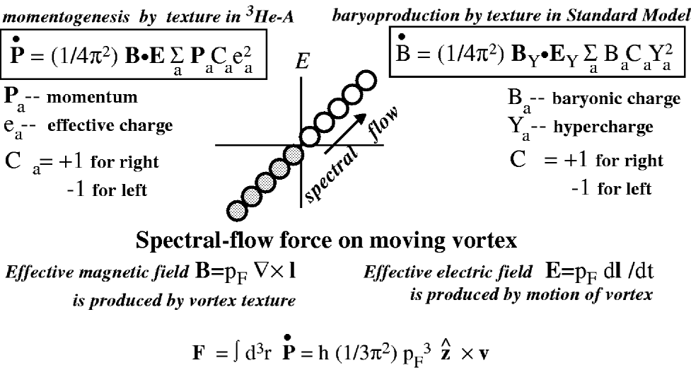
FIG. 9.: Production of the fermionic charge in ³He-A (linear momentum) and in Standard Model (baryonic number) are described by the same Adler-Bell-Jackiw equation. Integration of the anomalous momentum production over the cross-section of the moving continuous vortex gives the loss of linear momentum and thus the additional force per unit length acting on the vortex due to spectral flow.

Here we are interested in the process of the momentum transfer from the texture to quasiparticles. It can be described in terms of the chiral anomaly, since as we know the $\hat{\bf l}$ texture plays the part of the $U(1)$ effective gauge field acting on relativistic quasiparticles, and these quasiparticles are chiral. Thus we have all the conditions to apply the axial anomaly equation (130) to this process of transformation of the fermionic charge carried by magnetic field (texture) to the fermionic charge carried by chiral particles (normal component) (Fig.9). When a chiral quasiparticle crosses zero energy in its spectral flow it carries with it its linear momentum ${\cal{\bf P}}=\pm p_{F}\hat{\bf l}$. That is why this ${\cal{\bf P}}$ is the proper fermionic charge $q$ which enters the Eq.(130), and the rate of the momentum production from the texture is

$${\dot{\bf P}}={1\over 4\pi^{2}}\left({\cal{\bf P}}{\cal E}^{2},{\cal N}\right){\bf B}\cdot{\bf E}={1\over 4\pi^{2}}{\bf B}\cdot{\bf E}\sum_{a}{\bf P}_{a}C_{a}e_{a}^{2}~{}.$$ (137)

Here ${\bf B}=(p_{F}/\hbar)\nabla\times\hat{\bf l}$ and ${\bf E}=(p_{F}/\hbar)\partial_{t}\hat{\bf l}$ are effective “magnetic” and “electric” fields; ${\cal E}$ is the matrix of corresponding “electric” charges in Eq.(97): $e_{a}=-C_{a}$ (the “electric” charge is opposite to the chirality of the ³He-A quasiparticle); and ${\bf P}_{a}=-C_{a}p_{F}\hat{\bf l}$ is the momentum (fermionic charge) carried by the $a$-th fermionic quasiparticle. Using this translation to the ³He-A language one obtains that the momentum production from the texture per unit time per unit volume is

$${\dot{\bf P}}=-{p_{F}^{3}\over 2\pi^{2}\hbar^{2}}\hat{\bf l}\left(\partial_{t}\hat{\bf l}\cdot(\nabla\times\hat{\bf l})\right)~{}.$$ (138)

It is interesting to follow the hystory of this term in ³He-A. First the nonconservation of the momentum of the superfluid vacuum at $T=0$ has been found from the general consideration of the superfluid hydrodynamics of the vacuum [80]. Later it was found that the quasiparticles must be nucleated whose momentum production rate is described by the same Eq.(138), but with the opposite sign [81]. Thus the total momentum of the system has been proved to conserve. In the same paper Ref.[81] it was first found that the quasiparticle states in ³He-A in the presense of twisted texture of $\hat{\bf l}$ has strong analogies with the eigenstates of a charged particle in a magnetic field. Then it became clear [82] that the momentum production is described by the same equation as the axial anomaly in relativistic quantum field theory. Now we know why it happens: The spectral flow from the texture to the “matter” occurs through the Fermi point and thus it can be described by the physics in the vicinity of the Fermi point, where the “relativistic” quantum field theory necessarily arises.

D Axial anomaly and force on ³He-A vortices.

From the underlying microscopic theory we know that the total linear momentum of the liquid is conserved. The Eq. (138) thus implies that in the presence of a time-dependent texture the momentum is transferred from the texture (the distorted superfluid vacuum or magnetic field) to the heat bath of quasipartcles (analogue of matter). The rate of the momentum transfer gives an extra force acting on a moving $\hat{\bf l}$-texture. This force influences the dynamics of the continuous textures, which represents the vortex in ³He-A (analog of stringy texture in the Standard Model [83]), and this force has been measured in experiments on the rotating ³He-A [38] (see Sec. VII E).

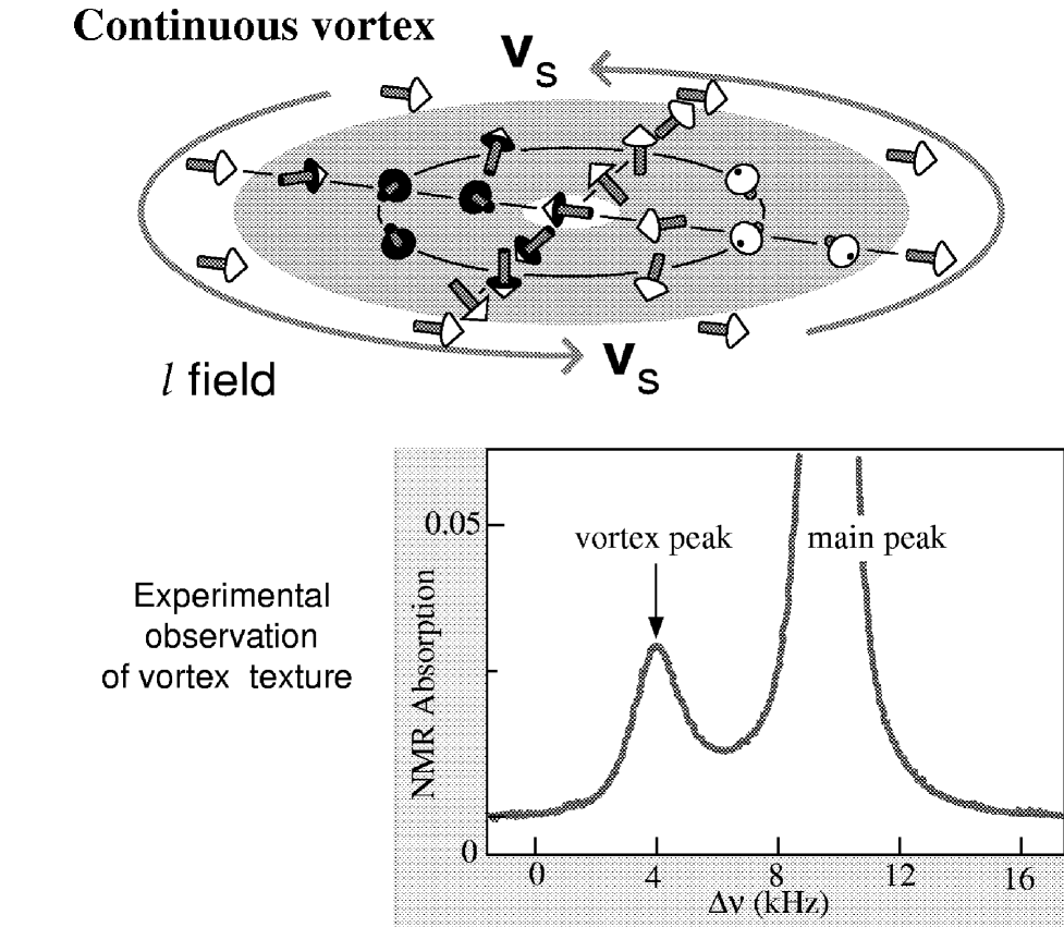
FIG. 10.: Top: An $n_{1}=2$ continuous vortex in ³He-A. The arrows indicate the local direction of the order parameter vector ${\hat{\bf l}}$. Under experimental conditions the direction of the ${\hat{\bf l}}$-vector in the bulk liquid far from the soft core is kept in the plane perpendicular to applied magnetic field far from the core. This does not change the topology of the Anderson-Toulouse-Chechetkin vortex: the ${\hat{\bf l}}$-vector covers the whole $4\pi$ sphere within the soft core. As a result there is $4\pi$ winding of the phase of the order parameter around the soft core, which corresponds to $n_{1}=2$ quanta of anticlockwise circulation. Bottom: The NMR absorption in the characteristic vortex satellite originates from the soft core where the ${\hat{\bf l}}$ orientation deviates from the homogeneous alignment in the bulk. Each soft core contributes equally to the intensity of the satellite peak and gives a practical tool for measuring the number of vortices.

The continuous vortex texture, first discussed by Chechetkin [84] and Anderson and Toulouse[85] (ATC vortex, Fig. 10), has in its simplest realization the following distribution of the ${\hat{\bf l}}$-field ($\hat{\bf z}$, ${\hat{\bf\rho}}$ and ${\hat{\bf\phi}}$ are unit vectors of the cylindrical coordinate system)

$${\hat{\bf l}}(\rho,\phi)={\hat{\bf z}}\cos\eta(\rho)+{\hat{\bf r}}\sin\eta(\rho)~{},$$ (139)

where $\eta(\rho)$ changes from $\eta(0)=0$ to $\eta(\infty)=\pi$. Such ${\hat{\bf l}}$-texture forms the so called soft core of the vortex, since it contains nonzero vorticity of superfluid velocity in Eq.(100):

$${\bf v}_{\rm s}(\rho,\phi)={\hbar\over 2m_{3}\rho}[1-\cos\eta(\rho)]{\hat{\bf\phi}}~{}~{},$$ (140)

In comparison to a more familiar singular vortex, the continuous vortex has a regular superfluid velocity field, with no singularity on the vortex axis, but the circulation of the superfluid velocity about the soft core is still quantized: $\oint d{\bf x}\cdot{\bf v}_{\rm s}=\kappa$ with $\kappa=2\pi\hbar/m$, which is twice the conventional circulation quantum number in the paircorrelated system $\kappa_{0}=2\pi\hbar/2m$, where $2m$ is the mass of the Cooper pair. Quantization of circulation in continuous vortex is related to the topology of the ${\hat{\bf l}}$-field: according to Mermin-Ho relation (101) the ${\hat{\bf l}}$-vector covers the whole $4\pi$ sphere when the soft core is swept.

The stationary vortex has nonzero effective “magnetic” field, ${\bf B}=(p_{F}\hbar)\nabla\times{\hat{\bf l}}$. If the vortex moves with a constant velocity ${\bf v}_{\rm L}$ with respect to the heat bath the moving texture acquires the time dependence, ${\hat{\bf l}}({\bf r}-{\bf v}_{\rm L}t)$, and this leads to the effective “electric” field

$${\bf E}={1\over\hbar}\partial_{t}{\bf A}=-{p_{F}\over\hbar}({\bf v}_{\rm L}\cdot{\bf\nabla}){\hat{\bf l}}$$ (141)

The net production of the quasiparticle momenta by the spectral flow in the moving vortex means: If the vortex moves with respect to the system of quasiparticles (the normal component of liquid or matter, whose flow is characterised by the normal velocity ${\bf v}_{\rm n}$), that there is a force acting between the normal component and the vortex. Integration of the anomalous momentum transfer in Eq.(138) over the cross-section of the soft core of the moving ATC vortex gives the following force acting on the vortex (per unit length) from the system of quasiparticles [86]:

$${\bf F}_{sf}=\int d^{2}\rho{p_{F}^{3}\over{2\pi^{2}\hbar^{2}}}\hat{\bf l}~{}(\partial_{t}\hat{\bf l}\cdot(\nabla\times\hat{\bf l}))=\int d^{2}\rho{p_{F}^{3}\over{2\pi^{2}\hbar^{2}}}\hat{\bf l}~{}((({\bf v}_{\rm n}-{\bf v}_{\rm L})\cdot\nabla)\hat{\bf l}\cdot(\nabla\times\hat{\bf l}))=-2\pi\hbar C_{0}{\hat{\bf z}}\times({\bf v}_{\rm L}-{\bf v}_{\rm n}),$$ (142)

where

$$C_{0}={p_{F}^{3}\over 3\pi^{2}\hbar^{3}}~{}.$$ (143)

Note that this spectral-flow force is transverse to the relative motion of the vortex and thus is nondissipative (reversible). In this derivation it was assumed that the quasiparticles and their momenta, created by the spectral flow from the vacuum, are finally absorbed by the normal component. The retardation in the process of absorption and also the viscosity of the normal component lead to a dissipative (friction) force between the vortex and the normal component: ${\bf F}_{fr}=-\gamma({\bf v}_{L}-{\bf v}_{\rm n})$. There is no momentum exchange between the vortex and the normal component if they move with the same velocity. The result (142) for the spectral-flow force, was also confirmed in a microscopic theory [87].

The important property of the spectral-flow force (142) is that it does not depend on the details of the vortex structure: The result for ${\bf F}_{sf}$ is robust against any deformation of the ${\hat{\bf l}}$-texture which does not change its asymptote, i.e. the topology of the vortex. In this respect this force resembles another force, the force between the vortex texture and the superfluid vacuum, which acts on the vortex moving with respect to the superfluid vacuum. This is the well-known Magnus force:

$${\bf F}_{M}=2\pi\hbar n{\hat{\bf z}}\times({\bf v}_{L}-{\bf v}_{\rm s}(\infty))~{},$$ (144)

where again $n$ is the particle density – the number density of ³He atoms; ${\bf v}_{\rm s}(\infty)$ is the uniform velocity of the superfluid vacuum far from the vortex.

Let us recall that the vortex texture (or quantized vortex in $U(1)$ superfluids) serve as mediator (intermediate object) for the momentum exchange between the superfluid vacuum and the fermionic heat bath of quasiparticles. The momentum is transferred from the vacuum to texture (this produces the Magnus force acting on the vortex texture) and then from the texture to the “matter” (with minus sign the spectral-flow force in Eq.(142) acting on the vortex texture from the system of quasiparticles). In this respect the texture (or vortex) corresponds to the sphaleron or to the cosmic string in relativistic theories. If the other processes are neglected then in the steady state these two forces acting on the texture from vacuum and “matter” must compensate each other. From this balance of the two forces one obtains that the vortex must move with the constant velocity determined by the velocities ${\bf v}_{\rm s}$ and ${\bf v}_{\rm n}$ of vacuum and matter: ${\bf v}_{L}=(n{\bf v}_{\rm s}-C_{0}{\bf v}_{\rm n})/(n-C_{0})$. However this is valid only under special conditions. Firstly the dissipative friction must be taken into account. It comes in particular from the retardation of the spectral flow process. The retardation also modifies the nondissipative spectral flow force. Secondly the analogy with the gravity shows that there is one more force of topological origin – the so-called Iordanskii force in Eq.(XII B). It comes from the gravitational analog of the Aharonov-Bohm effect experienced by particles moving in the presence of the spinning cosmic string (see Sec.XII B).

E Experimental verification of Adler-Bell-Jackiw equation in rotating ³He-A.

The spectral flow force acting on the vortex has been measured in experiments on vortex dynamics in ³He-A [38, 88]. In such experiments a uniform array of vortices is produced by rotating the whole cryostat. In equilibrium the vortices and the normal component of the fluid (heat bath of quasiparticles) rotate together with the cryostat. An electrostatically driven vibrating diaphragm produces an oscillating superflow, which via the Magnus force generates the vortex motion, while the normal component remains clamped due to its high viscosity. This creates a motion of vortices with respect both to the heat bath (“matter”) and the superfluid vacuum. The vortex velocity ${\bf v}_{L}$ is determined by the overall balance of forces acting on the vortices. This includes the spectral flow force ${\bf F}_{sf}$ in Eq.(142); the Magnus force ${\bf F}_{M}$ in Eq.(144); the friction force ${\bf F}_{fr}=-\gamma({\bf v}_{L}-{\bf v}_{\rm n})$; and the Iordanskii force in Eq.(XII B) coming from the gravitational analog of the Aharonov-Bohm effect (see Sec.XII B). For the doubly quantized vortex the Iordanskii force is

$${\bf F}_{\rm Iordanskii}=2\pi\hbar n_{\rm n}{\hat{\bf z}}\times({\bf v}_{\rm s}(\infty)-{\bf v}_{\rm n})~{},$$ (145)

where the momentum carried by quasiparticles is expressed in terms of the normal component density: $\sum_{\bf p}{\bf p}f({\bf p})=mn_{\rm n}({\bf v}_{\rm s}(\infty)-{\bf v}_{\rm n})$. Since for the steady state motion of vortices the sum of all forces acting on the vortex must be zero, ${\bf F}_{M}+{\bf F}_{sf}+{\bf F}_{\rm Iordanskii}+{\bf F}_{fr}=0$, one has the following equation for ${\bf v}_{L}$:

$$\hat{\bf z}\times({\bf v}_{L}-{\bf v}_{\rm s}(\infty))+d_{\perp}\hat{\bf z}\times({\bf v}_{\rm n}-{\bf v}_{L})+d_{\parallel}({\bf v}_{\rm n}-{\bf v}_{L})=0~{}~{},$$ (146)

where

$$d_{\perp}=1-{n-C_{0}\over n_{\rm s}(T)}~{},$$ (147)

$n_{\rm s}(T)=n-n_{\rm n}(T)$ is the density of the superfluid component; and $d_{\parallel}=\gamma/2\pi n_{\rm s}$.

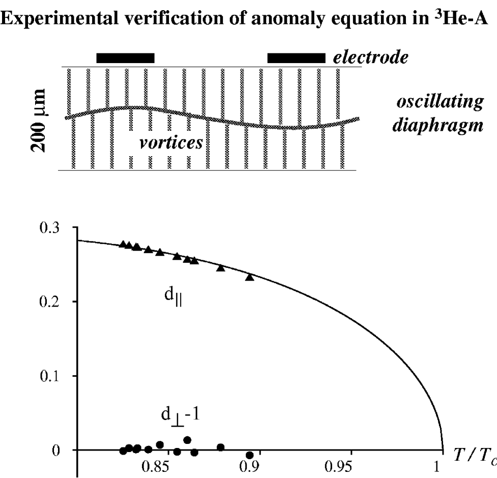
FIG. 11.: A uniform array of vortices is produced by rotating the whole cryostat, and oscillatory superflow perpendicular to the rotation axis is produced by a vibrating diaphragm, while the normal fluid (thermal excitations) is clamped by viscosity, ${\bf v}_{\rm n}=0$. The velocity ${\bf v}_{L}$ of the vortex array is determined by the overall balance of forces acting on the vortices. These vortices produce additional dissipation proportional to $d_{\parallel}$ and coupling between two orthogonal modes proportional to $1-d_{\perp}$.

Measurement of the damping of the diaphragm resonance and of the coupling between different eigenmodes of vibrations enables both dimensionless parameters, $d_{\perp}$ and $d_{\parallel}$, to be deduced. The most important for us is the parameter $d_{\perp}$, which gives information on the spectral flow parameter $C_{0}$. The effect of the chiral anomaly is crucial for $C_{0}$: If there is no anomaly then $C_{0}=0$ and $d_{\perp}=n_{\rm n}(T)/n_{\rm s}(T)$; if the anomaly is fully realized the parameter $C_{0}$ has its maximal value, $C_{0}=p_{F}^{3}/3\pi^{2}\hbar^{3}$, which coincides with the particle density of liquid ³He in the normal state, Eq.(62). The difference between the particle density of liquid ³He in the normal state $C_{0}$ and the particle density of liquid ³He in superfluid ³He-A state $n$ at the same chemical potential $\mu$ is determined by the tiny effect of superfluid correlations on the particle density and is extremely small: $n-C_{0}\sim n(\Delta_{0}/v_{F}p_{F})^{2}=n(c_{\perp}/c_{\parallel})^{2}\sim 10^{-6}n$; in this case one must have $d_{\perp}\approx 1$ for all practical temperatures, even including the region close to $T_{c}$, where the superfluid component $n_{s}(T)\sim n(1-T^{2}/T_{c}^{2})$ is small. ³He-A experiments, made in the whole temperature range where ³He-A is stable, gave precisely this value within experimental uncertainty, $|1-d_{\perp}|<0.005$[38] (see Fig. 11).

This means that the anomaly is fully realized in the dynamics of the $\hat{\bf l}$ texture and provides an experimental verification of the Adler-Bell-Jackiw axial anomaly equation (130), applied to ³He-A. This supports the idea that baryonic charge (as well as leptonic charge) can be generated by electroweak gauge fields through the anomaly.

In the same experiments with the ³He-B vortices the effect analogous to the axial anomaly is temperature dependent and one has the crossover from $d_{\perp}\approx 1$ at high $T$ to $d_{\perp}=n_{\rm n}(T)/n_{\rm s}(T)$ at low $T$ (see Sec. IX B 2 and Fig. 17). The reason for that is that Eq. (130) for axial anomaly and the corresponding equation (138) for the momentum production are valid only in the limit of continuous spectrum, i.e. when the distance $\omega_{0}$ between the energy levels of fermions in the texture is much smaller than the inverse quasiparticle lifetime: $\omega_{0}\tau\ll 1$. The spectral flow completely disappears in the opposite case $\omega_{0}\tau\gg 1$, because the spectrum becomes effectively discrete. As a result, the force acting on a vortex texture differs by several orders of magnitude for the cases $\omega_{0}\tau\ll 1$ and $\omega_{0}\tau\gg 1$. The parameter $\omega_{0}\tau$ is regulated by temperature. In case of ³He-A the vortices are continuous and thus $\omega_{0}$ is extremely small and can be negelected. This means that the spectral flow is maximally possible and thus the Adler-Bell-Jackiw anomaly equation is applicable there for all practical temperatures and it was experimentally confirmed.

Note in conclusion of this Section, that the spectral flow in vortices realizes the momentum exchange between the 3+1 fermionic system outside the vortex and the 1+1 fermions living in the vortex core. This corresponds to the Callan-Harvey process of anomaly cancellation [89] between the systems of different dimension [90, 91] (see also Sec. IX B).

VIII Macroscopic parity violating effects.

A Helicity in parity violating systems.

Parity violation, the asymmetry between left and right, is one of the fundamental properties of the quantum vacuum. This effect is strong at high energy of the order of electroweak scale, but is almost imperceptible in the low-energy condensed matter physics. Since at this scale the left and right particles are hybridized and only the left-right symmetric charges survive. For example, Leggett’s suggestion to observe the macroscopic effect of parity violation using such macroscopically coherent atomic system as superfluid ³He-B is very far from realization [92, 13]. On the other hand, an analog of parity violation exists in superfluid ³He-A alongside with the related phenomena, such as chiral anomaly which we discussed in previous section and macroscopic chiral currents (for a review see Refs. [13, 40]). So, if we cannot investigate the macroscopic parity violating effects directly we can simulate analogous physics in ³He-A.

Most of the macroscopic parity violating phenomena are related to helicity: the energy of the system in which the parity is broken contains the helicity term $\lambda{\bf A}\cdot({\bf\nabla}\times{\bf A})$, where ${\bf A}$ is the relevant collective vector field. To have such terms the parity $P$ must be violated together with all the combinations containing other descrete symmetries, such as $CP$, $PT$, $CPT$, $PU_{2}$ (where $U_{2}$ is the rotation by $\pi$), etc. Such terms sometimes lead to the instability of the vacuum towards the spacially inhomogeneous state, the helical instability. In nematic liquid crystals, for example, the excess of the chiral molecules of one preferred chirality leads to the helicity term, $\lambda\hat{\bf n}\cdot({\bf\nabla}\times\hat{\bf n})$, for the nematic vector (director) field ${\hat{\bf n}}$. This leads to formation of the cholesteric structure, the helix. The same phenomenon occurs in superfluid ³He-A, where at some conditions there is a helical instability of the homogeneous counterflow ${\bf w}={\bf v}_{\rm n}-{\bf v}_{\rm s}$, which we discuss in this Section. The interest to this instability arises because it is the counterpart of the helical instability of an excess of the massless right-handed electrons over the left-handed, which leads to formation of the helical hypermagnetic field ${\bf B}_{Y}$ [93, 94]. The formed field ${\bf B}_{Y}$, after the electroweak transition occurs, is transformed to electromagnetic magnetic field ${\bf B}(={\bf B}_{Q})$. Thus the helical instability can be the source of formation of primordial cosmological magnetic fields (see also recent review paper on cosmic magnetic fields [95] and references therein).

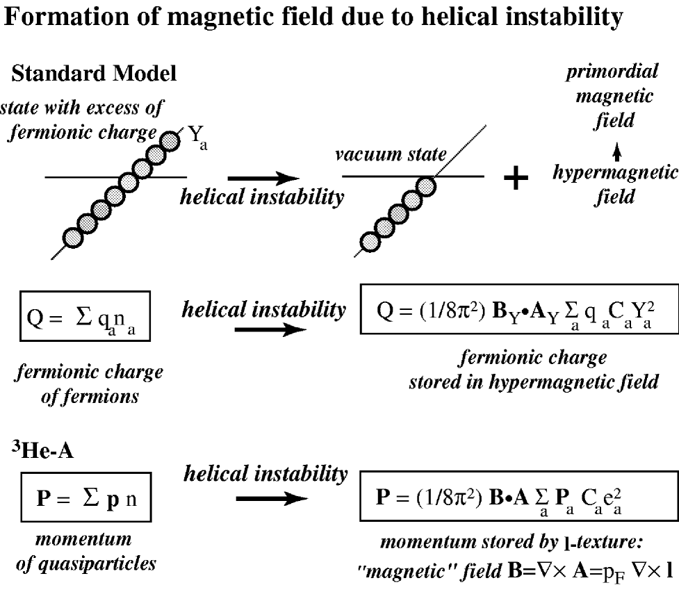
FIG. 12.: The fermionic charge of right-handed minus that of left-handed particles is conserved at the classical level but not if quantum properties of the physical vacuum are taken into account. This charge can be transferred to the “inhomogeneity” of the vacuum via the axial anomaly in the process of the helical instability. The inhomogeneity which absorbs the fermionic charge arises as a hypermagnetic field configuration in the Standard Model and as the ${\hat{\bf l}}$-texture in ³He-A, which is analogous to the magnetic field.

Here we show that the helical instability of the counterflow in ³He-A and the helical instability of the system of the right electrons with nonzero chemical potential are the same phenomena and thus are described by the same effective action, which contains the Chern-Simons helical term (Fig.refPrimordialMagnField1Fig).

B Chern-Simons energy term.

1 Chern-Simons term in Standard Model.

Due to axial anomaly fermionic charge, say, baryonic or leptonic, can be transferred to the “inhomogeneity” of the vacuum. This inhomogeneity, which absorbs the fermionic charge, arises as a helix of magnetic field configuration, say, hypermagnetic field. According to axial anomaly equation (131), the fermionic charge $Q$ absorbed by the hypermagnetic field, is

$$Q\{{\bf A}_{Y}\}={1\over 2\pi^{2}}\left({\cal Q}{\cal Y}^{2},{\cal N}\right){\bf A}_{Y}\cdot({\bf\nabla}\times{\bf A}_{Y})~{}~{}.$$ (148)

Let us recall that for the noninteracting fermions this equations reads

$$Q\{{\bf A}_{Y}\}={1\over 2\pi^{2}}{\bf A}_{Y}\cdot({\bf\nabla}\times{\bf A}_{Y})\sum_{a}C_{a}Q_{a}Y_{a}^{2}~{}~{},$$ (149)

where again $a$ marks the fermionic species; $C_{a}=\pm 1$ is the chirality of the fermion; $Y_{a}$ and $Q_{a}$ are correspondingly the hypercharge of the $a$-th fermion and its relevant fermionic charge, whose absorption by the hyperfield we discuss. The fermionic charge which we interested in is the fermionic number $Q_{a}=3B_{a}+L_{a}$.

If the fermions are non interacting and their chemical potentials $\mu_{a}$ are nonzero, then the energy functional contains the term which describes the conservation of $3B_{a}+L_{a}$,

$$-\sum_{a}\mu_{a}n_{a}~{}~{},~{}~{}n_{a}=n_{a}^{\rm fermion}+n_{a}\{{\bf A}_{Y}\}~{}.$$ (150)

Here $n_{a}$ is the total charge density $3B_{a}+L_{a}$, which is the sum of the charge density $n_{a}^{\rm fermion}$ stored by the system of fermionic quasiparticles and the charge density $n_{a}\{{\bf A}_{Y}\}$ stored by the $U(1)_{Y}$ gauge field. The latter gives the Chern-Simons energy of the hypercharge $U(1)_{Y}$ field in the presence of nonzero $\mu_{a}$:

$$F_{CS}\{{\bf A}_{Y}\}=-\sum_{a}\mu_{a}n_{a}\{{\bf A}_{Y}\}=-{1\over 8\pi^{2}}{\bf A}_{Y}\cdot({\bf\nabla}\times{\bf A}_{Y})\sum_{a}C_{a}\mu_{a}Y_{a}^{2}~{}~{}.$$ (151)

As an example let us consider the unification scale, where all the fermions have the same chemical potential $\mu$, since they can transform to each other at this scale. From the generating function for the Standard Model in Eq.(118) one has $\sum_{a}C_{a}Y_{a}^{2}=\left({\cal Y}^{2},{\cal N}\right)=2N_{F}$ and thus the Chern-Simons energy of the hypercharge field at high energy becomes:

$$F_{CS}\{{\bf A}_{Y}\}=-{\mu N_{F}\over 4\pi^{2}}{\bf A}_{Y}\cdot({\bf\nabla}\times{\bf A}_{Y})~{}~{}.$$ (152)

2 Chern-Simons energy in ³He-A.

Let us consider homogeneous counterflow ${\bf w}={\bf v}_{\rm n}-{\bf v}_{\rm s}=w\hat{\bf z}$. As will be clear below in Eq.(159), at nonzero $T$ the counterflow orients the ${\hat{\bf l}}$ vector along the axis of the counterflow, so that the equilibrium orientations of the ${\hat{\bf l}}$ field are ${\hat{\bf l}}_{0}=\pm{\hat{\bf z}}$. Since ${\hat{\bf l}}$ is a unit vector, its variation $\delta{\hat{\bf l}}\perp{\hat{\bf l}}_{0}$. In the gauge field analogy, in which ${\bf A}=p_{F}\delta{\hat{\bf l}}$, this corresponds to the gauge choice ${\bf A}^{3}=0$.

In the presence of counterflow the energy of quasiparticles, which enters the equilibrium distribution function in Eq.(9), is Doppler shifted by an amount $-{\bf p}\cdot{\bf w}$, which is $\approx C_{a}p_{F}({\hat{\bf l}}\cdot{\bf w})$ near the two nodes. The distribution function of the low-energy quasiparticles, i.e. in the vicinity of nodes, acquires the form

$$f_{a}({\bf p})=\left(\exp{E({\bf p})-\mu_{a}\over T}\pm 1\right)^{-1}~{},$$ (153)

where the effective chemical potential produced by the counterflow:

$$\mu_{a}=-C_{a}p_{F}({\hat{\bf l}}\cdot{\bf w})~{}~{}.$$ (154)

$\mu_{a}$ is the effective chemical potential for quasiparticles. This is distinct from the chemical potential $\mu$, which is the true chemical potential of the original bare particles, atoms of the underlying liquid, ⁴He atoms in Sec.II and ³He atoms in Sec.IV. The latter arises from the microscopic physics as a result of the conservation of number of atoms. The effective chemical potential $\mu_{a}$ for quasiparticles appears only in the low energy corner, i.e. in the vicinity of the $a$-th node, since in general there is no conservation law for the quasiparticles.

The relevant fermionic charge of ³He-A, which is anomalously conserved and which corresponds to the number of fermions, is as in Eq.(137) the momentum of quasiparticles along ${\hat{\bf l}}$, i.e. ${\bf P}_{a}=-C_{a}p_{F}{\hat{\bf l}}$. According to our analogy the helicity of the effective gauge field ${\bf A}=p_{F}{\hat{\bf l}}$ must carry the following linear momentum

$${\bf P}\{{\bf A}\}={1\over 8\pi^{2}}{\bf A}\cdot({\bf\nabla}\times{\bf A})\sum_{a}C_{a}{\bf P}_{a}e_{a}^{2}=-{p_{F}^{3}\over 4\pi^{2}}{\hat{\bf l}}\left(\delta{\hat{\bf l}}\cdot({\bf\nabla}\times\delta{\hat{\bf l}})\right)~{}~{}.$$ (155)

The total linear momentum of quasiparticles stored both in the heat bath of quasiparticles (“matter”) and in the texture (“hyperfield”) is thus

$${\bf P}={\bf P}^{\rm fermion}+{\bf P}^{\rm texture}~{}=\sum_{\bf p}{\bf p}f({\bf p})+{\bf P}\{{\bf A}\}~{}~{}.$$ (156)

The kinetic energy of the liquid in the presence of the counterflow contains the term which is equivalent to Eq.(150)

$$-({\bf v}_{\rm n}-{\bf v}_{\rm s}){\bf P}=-{\bf w}\sum_{\bf p}{\bf p}f({\bf p})-{\bf w}{\bf P}\{{\bf A}\}~{}~{}.$$ (157)

The second term in the rhs is precisely the analogue of the Chern-Simons energy in Eq.(151), which is now stored by the ${\hat{\bf l}}$ field in the presence of the counterflow:

$$F_{CS}\{\delta{\hat{\bf l}}\}=-{1\over 8\pi^{2}}{\bf A}\cdot({\bf\nabla}\times{\bf A})\sum_{a}C_{a}\mu_{a}e_{a}^{2}\equiv-{p_{F}^{3}\over 4\pi^{2}}({\hat{\bf l}}\cdot{\bf w})\left(\delta{\hat{\bf l}}\cdot({\bf\nabla}\times\delta{\hat{\bf l}})\right)~{}~{}.$$ (158)

3 Kinetic energy of counterflow in ³He-A and its analog for chiral fermions.

The first term in the rhs of Eq.(157) together with the quasiparticle energy $\sum_{\bf p}E({\bf p})f({\bf p})$ gives:

$${7\pi^{2}\over 180}{m^{*}p_{F}\over\Delta_{0}^{2}}T^{4}-{1\over 2}mn_{{\rm n}\parallel}({\bf w}\cdot{\hat{\bf l}})^{2}~{}.$$ (159)

While the first term is the thermal energy of the gapless fermions, the second term in Eq.(159) is with the minus sign the kinetic energy of the counterflow. Here $n_{{\rm n}\parallel}$ is the density of the normal component for the flow along ${\hat{\bf l}}$ (see Eq.(10) in Sec.II C):

$$n_{{\rm n}ik}=n_{{\rm n}\parallel}\hat{l}_{i}\hat{l}_{k}+n_{{\rm n}\perp}(\delta_{ik}-\hat{l}_{i}\hat{l}_{k})~{}~{},~{}~{}n_{{\rm n}\parallel}\approx{m^{*}\over 3m}p_{F}^{3}{T^{2}\over\Delta_{0}^{2}}~{}~{}.$$ (160)

It is the second term in Eq.(159) which provides the preferred orientation of the ${\hat{\bf l}}$ field by the counterflow velocity. As will be shown in Sec.VIII B 4 below it is responsible for the mass of the gauge field boson.

The Eq.(159) can be written in the relativistic form applicable both for ³He-A and the system of chiral fermions:

$$\Omega(T,\mu_{a})=\Omega(T,0)+\Omega^{\prime}(T,\mu_{a})={7\pi^{2}\over 180}\sqrt{-g}T^{4}\sum_{a}1-{\sqrt{-g}\over 12}T^{2}\sum_{a}\mu_{a}^{2}~{},$$ (161)

where in ³He-A the determinant of the metric tensor $g_{\mu\nu}$ is according to Eq.(106):

$$\sqrt{-g}={1\over c_{\parallel}c_{\perp}^{2}}={m^{*}p_{F}\over\Delta_{0}^{2}}~{}~{}.$$ (162)

In relativistic system the second term $\Omega^{\prime}(T,\mu_{a})$ in Eq.(161) is the correction to the thermodynamic potential due to the chemical potential if $\mu_{a}^{2}\ll T^{2}$. In derivation of Eq.(159) we also used the condition $\mu_{a}^{2}\ll T^{2}$, which corresponds to $p_{F}w\ll T$. Under this condition the thermal energy, which is $\propto\sqrt{-g}T^{4}$ in both systems, is dominating. The minus sign in the kinetic energy of quasiparticles in Eq.(159) occurs since the counterflow velocity ${\bf w}$ is kept fixed. This corresponds to the minus sign in the relativistic version, Eq.(161), where the chemical potentials are kept fixed.

4 Mass of hyperphoton.

Another term which is important for the consiferation of the helical instability in ³He-A is that which gives the mass of “hyperphoton”. This mass can be obtained from Eq.(159) by expanding the unit vector ${\hat{\bf l}}$ up to the second order in deviations: ${\hat{\bf l}}={\hat{\bf l}}_{0}+\delta{\hat{\bf l}}-(1/2){\hat{\bf l}}_{0}(\delta{\hat{\bf l}})^{2}$. Inserting this equation to Eq.(159) and neglecting the terms which does not contain the $\delta{\hat{\bf l}}$ field one obtains the term whose translation to the relativistic language gives the mass for the $U(1)_{Y}$ gauge field:

$$F_{\rm mass}={1\over 4}mn_{{\rm n}\parallel}w^{2}(\delta{\hat{\bf l}}\cdot\delta{\hat{\bf l}})$$ (163)

$$\equiv{1\over 12}\sqrt{-g}g^{ik}A_{i}A_{k}{T^{2}\over\Delta_{0}^{2}}\sum_{a}e_{a}^{2}\mu_{a}^{2}~{}~{}.$$ (164)

In ³He-A this mass of the “hyperphoton” is physical and important for the dynamics of the $\hat{\bf l}$-vector. It is the gap in the spectrum of orbital waves – propagating oscillations of $\delta\hat{\bf l}$. This mass appears due to the presence of the counterflow, which orients $\hat{\bf l}$ and thus provides the restoring force for oscillations of $\delta\hat{\bf l}$.

In principle, the similar mass can exist for the real hyperphoton. If the Standard Model is an effective theory, the local $U(1)_{Y}$ symmetry arises only in the low-energy corner and thus is approximate. It can be violated (not spontaneously but gradually) by the higher order terms, which contain the Planck cut-off. Let us recall that the cut-off parameter $\Delta_{0}$ does play the part of the Planck energy scale. The Eq. (164) suggests that the mass of the hyperphoton could arise if both the temperature $T$ and the chemical potential $\mu_{a}$ are finite. This mass disappears in the limit of an infinite cut-off parameter or is negligibly small, if the cut-off is of Planck scale $E_{\rm P}$. The ³He-A thus provides an illustration of how the renormalizable terms are suppressed by small ratio of the energy to the fundamental energy scale of the theory [3] and how the terms of order $(T/E_{\rm P})^{2}$ appear in the effective quantum field theory [4].

On the other hand, the mass term can be obtained in the effective theory too, if one relates its to the gravity, which is also determined by the Planck energy scale. The nonzero chemical potential in Eq.(161) gives the nonzero trace of energy momentum tensor for quasiparticles (matter) according to Eq.(48):

$$~{}T^{\mu}{}_{\mu}=2\Omega^{\prime}(T,\mu_{a})~{}.$$ (165)

Using the Einstein equation, $R=-8\pi GT^{\mu}{}_{\mu}$, the Eq.(164) can be transformed to

$$F_{\rm mass}={1\over 16\pi G\Delta_{0}^{2}}\sqrt{-g}g^{ik}A_{i}A_{k}R{\sum_{a}e_{a}^{2}\mu_{a}^{2}\over\sum_{a}\mu_{a}^{2}}~{}~{}.$$ (166)

The microscpic parameters $\Delta_{0}^{2}$ and $G\sim\Delta_{0}^{-2}$ cancel each other, so that no cut-off parameter enters the mass term. This effective action is general covariant and scale invariant but it violates the gauge symmetry. Applying this for the hypermagnetic field ${\bf A}_{Y}$ with charges $e_{a}=Y_{a}$, and identifying $G\Delta_{0}^{2}=GE_{\rm P}^{2}=1$ one obtains for the case of equal chemical potentials:

$$F_{\rm mass}={5\over 24}{1\over 16\pi}\sqrt{-g}g^{\mu\nu}A_{\mu Y}A_{\nu Y}R~{}~{}.$$ (167)

In principle the term $\sqrt{-g}T^{4}g^{ik}A_{i}A_{k}/E_{\rm P}^{2}$ is also possible, which gives the hyperphoton mass of order $T^{2}/E_{\rm Planck}$.

C Helical instability and “magnetogenesis” by chiral fermions.

The Chern-Simons term in Eqs. (151) and (158) is odd under spatial parity tranformation and thus can have a negative sign for the properly chosen field or texture. Thus one can have an energy gain from the transformation of the fermionic charge to the $U(1)$ gauge field. This is the essence of the Joyce-Shaposhnikov scenario for the generation of primordial magnetic field [93, 94]. In ³He-A language this process describes the collapse of the counterflow, where the relevant fermionic charge is the momentum, towards the formation of ${\hat{\bf l}}$-texture. Such a collapse of quasiparticle momentum was recently observed in the rotating cryostat of the Helsinki Low Temperature Laboratory [96, 10] (Fig. 13).

1 Helical instability condition.

The instability can be found by investigation of the eigenvalues of the quadratic form describing the energy in terms of the deviations from the homogeneous counterflow, which play the part of the “hypermagnetic” field ${\bf A}=p_{F}\delta{\hat{\bf l}}$. The quadratic form contains Eqs. (125), (158), and (163) describing correspondingly the “magnetic” energy, the Chern-Simons energy, and the term giving the mass of the “hyperphoton”. In ³He-A notations this is:

$${{12\pi^{2}}\over{p_{F}^{2}v_{F}}}F\{\delta{\hat{\bf l}}\}=(\partial_{z}\delta\hat{\bf l})^{2}{\rm ln}{\Delta_{0}\over T}-3m^{*}w\delta{\hat{\bf l}}\cdot(\hat{\bf z}\times\partial_{z}\delta{\hat{\bf l}})+\pi^{2}(m^{*}w)^{2}{T^{2}\over\Delta_{0}^{2}}(\delta{\hat{\bf l}})^{2}$$ (168)

or after the rescaling of the coordinates $\tilde{z}=zm^{*}w/\hbar$

$${4F\{\delta{\hat{\bf l}}\}\over C_{0}m^{*}w^{2}}=(\partial_{\tilde{z}}\delta\hat{\bf l})^{2}{\rm ln}{\Delta_{0}\over T}-3\delta{\hat{\bf l}}\cdot(\hat{\bf z}\times\partial_{\tilde{z}}\delta{\hat{\bf l}})+\pi^{2}{T^{2}\over\Delta_{0}^{2}}(\delta{\hat{\bf l}})^{2}$$ (169)

The quadratic form in Eq.(169) becomes negative and thus the uniform counterflow becomes unstable towards the nucleation of the $\hat{\bf l}$-texture if

$${T^{2}\over\Delta_{0}^{2}}\ln{\Delta_{0}\over T}<{9\over 4\pi^{2}}~{}~{}.$$ (170)

If this condition is fulfilled, the instability occurs for any value of the counterflow.

In relativistic theories, where the temperature is always smaller than the Planck cut-off $\Delta_{0}$, the condition corresponding to Eq.(170) is always fulfilled. Thus the excess of the fermionic charge is always unstable towards nucleation of the hypermagnetic field, if the fermions are massless, i.e. above the electroweak transition. In the scenario of the magnetogenesis developed by Joyce and Shaposhnikov [93, 94], this instability is responsible for the genesis of the hypermagnetic field well above the electroweak transition. The role of the subsequent electroweak transition is to transform this hypermagnetic field to the conventional (electromagnetic $U(1)_{Q}$) magnetic field due to the electroweak symmetry breaking.

2 Experimental “magnetogenesis” in rotating ³He-A.

In ³He-A the helical instability is suppressed by another mass of the “hyperphoton”, which comes from the spin-orbit interaction $-g_{D}({\hat{\bf l}}\cdot{\hat{\bf d}})^{2}$ between the orbital vector ${\hat{\bf l}}$ and the vector ${\hat{\bf d}}$, describing the spin part of the order parameter. This gives an additional restoring force acting on ${\hat{\bf l}}$, and thus the additional mass of the gauge field: $-g_{D}({\hat{\bf l}}\cdot{\hat{\bf d}})^{2}=-g_{D}({\hat{\bf l}}_{0}\cdot{\hat{\bf d}})^{2}+(1/2)g_{D}(\delta{\hat{\bf l}})^{2}$, which is independent on the counterflow. As a result the helical instability occurs only if the counterflow (the corresponding chemical potential $\mu_{a}$) exceeds the critical treshold, determined by the additional mass of the “hyperphoton”, which is of order $M_{\rm hp}\sim 10^{-3}\Delta_{0}$. This is observed experimentally [96] (see Fig.13). When the counterflow in the rotating vessel exceeds this treshold, the intensive formation of the ${\hat{\bf l}}$ texture by helical instability is detected by NMR. This corresponds to the formation of the hypermagnetic field according to our analogy. The only difference from the Joyce-Shaposhnikov scenario is that the mass of the “hyperphoton” provides the treshold for the helical instability.

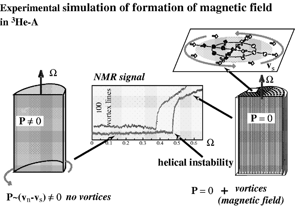
FIG. 13.: left) The vortex-free state in the vessel rotating with angular velocity ${\bf\Omega}$ contains a counterflow, ${\bf w}={\bf v}_{\rm n}-{\bf v}_{\rm s}={\bf\Omega}\times{\bf r}\neq 0$, since the average velocity of quasiparticles (the normal component) is ${\bf v}_{\rm n}={\bf\Omega}\times{\bf r}$ and is not equal to the velocity of the superfluid vacuum, which is at rest, ${\bf v}_{\rm s}=0$. In the counterflow state, the quasiparticles have a net momentum $\propto n_{\rm n}{\bf w}$. In the presence of counterflow ${\bf w}$, the energy of quasiparticles is Doppler shifted by the amount ${\bf p}\cdot{\bf w}\approx\pm p_{F}({\hat{\bf l}}_{0}\cdot{\bf w})$. The counterflow therefore produces what would be an effective chemical potential in particle physics. For right-handed particles, this is $\mu_{R}=p_{F}({\hat{\bf l}}_{0}\cdot{\bf w})$ and for left-handed particles it is $\mu_{L}=-\mu_{R}$. Thus rotation produces an excess of the fermionic charge quasiparticle momentum, which is analogous to the excess of the leptonic charge of chiral right-handed electrons if their chemical potential $\mu_{R}$ is nonzero. middle When the excess of quasiparticle momentum reaches the critical value, the helical instability occurs, which is marked by abrupt jump of the intensity of the NMR satellite peak from zero, which signals appearance of the ${\hat{\bf l}}$-texture, playing the part of the magnetic field. right The final result of the helical instability is a periodic array of continuous $n_{1}=2$ vortices (top). Formation of these vortices leads to the effective solid body rotation of superfluid vacuum with $<{\bf v}_{\rm s}>\approx{\bf\Omega}\times{\bf r}$. This essentially decreases the counterflow and thus the fermionic charge. Thus a part of the fermionic charge is transformed into “hypermagnetic” field.

In principle, however the similar treshold can appear in the Standard Model if there is a small “non-renormalizable” mass of the hyperphoton, $M_{\rm hp}$, produced by the Planck-scale physics. In this case the decay of the fermionic charge stops, and thus the excess of, say, the baryionic charge is not washed out any more, when the chemical potential of fermions becomes comparable with $M_{\rm hp}$. The observed baryon asymmetry would be achieved if the initial mass of the hyperhoton at the electroweak temperature, $T\sim E_{\rm ew}$, is $M_{\rm hp}\sim 10^{-9}E_{\rm ew}$. This is however too large compared with the possible hyperphoton mass, discussed earlier, which is of order $T^{2}/E_{\rm P}\sim E_{\rm ew}^{2}/E_{\rm P}$.

D Mixed axial-gravitational Chern-Simons term.

1 Parity violating current

The chiral anomaly problem can be mapped to the angular momentum paradox in ³He-A. To relate them let us consider the parity effects which occur for the rotating chiral fermions. The macroscopic parity violating effects in a rotating system with chiral fermions was first discussed by Vilenkin in Ref. [97]. The angular velocity of rotation ${\bf\Omega}$ defines the preferred direction of polarization, and right-handed fermions move in the direction of their spin. As a result, such fermions develop a current parallel to ${\bf\Omega}$. Similarly, left-handed fermions develop a current antiparallel to ${\bf\Omega}$. The corresponding current density was calculated in [97], assuming thermal equilibrium at temperature $T$ and chemical potential of the fermions $\mu$. For right-handed fermions, it is given by

$${\bf j}=\left({T^{2}\over{12}}+{\mu^{2}\over{4\pi^{2}}}\right){\bf\Omega}.$$ (171)

The current ${\bf j}$ is a polar vector, while the angular velocity ${\bf\Omega}$ is an axial vector, and thus Eq.(171) violates the reflectional symmetry.

If the current (171) is coupled to a gauge field $A^{\nu}$, the appropriate term in the Lagrangian density is

$$L={1\over c^{2}}{\bf\Omega}\cdot{\bf A}\left({T^{2}\over{12}}\sum_{a}e_{a}C_{a}+{1\over{4\pi^{2}}}\sum_{a}e_{a}C_{a}\mu_{a}^{2}\right)~{},$$ (172)

where $e_{a}$ are the corresponding couplings with the gauge field. Since the rotation can be described in terms of metric, this represents the mixed axial-gravitational Chern-Simons term in the effective action of Standard Model [98]. After expressing it in the covariant form, this term can be applied to ³He-A too.

2 Orbital angular momentum and free energy

Let us consider a stationary liquid ³He-A in a vessel rotating with angular velocity ${\bf\Omega}$ at a nonzero temperature. We assume a spatially homogeneous vector ${\hat{\bf l}}=\hat{\bf z}$ oriented along the rotation axis. In ³He-A this can be achieved in the parallel-plane geometry, while in the layered oxide superconductor Sr₂RuO₄, which is believed to be a triplet superconductor with a ³He-A-like order parameter, the ${\hat{\bf l}}$-vector is always fixed along the normal to the layers [99, 100]. The superfluid component (vacuum) is assumed to be at rest, ${\bf v}_{\rm s}=0$, while the normal component circulates in the plane perpendicular to $\hat{\bf l}$ performing the solid-body like rotation with the velocity ${\bf v}_{\rm n}={\bf\Omega}\times{\bf r}$. This state corresponds to the true thermodynamic equilibrium in rotating vessel, though it is rather local than global minumum of the thermodynamic potential in rotating frame. The absolute minimum would correspond to the system of quantized vortices in rotating vessel, but since the energy barrier between the states with different number of vortices is high, while the temperture is low, the probability of the thermally activating transitions between the states (as well as quantum tunneling) is less than $\exp(-10^{6})$. This is an advantage of superfluid ³He, which allows us to support the states with given number of vortices, including the vortex-free state [101].

The value of the angular momentum of a rotating ³He-A has been a subject of a long-standing controversy (for a review see [13, 40]). Different methods for calculating the angular momentum give results that differ by many orders of magnitude. The result is also sensitive to the boundary conditions, since the angular momentum in the liquid is not necessarily the local quantity, and to whether the state is strictly stationary or has a small but finite frequency. This is often referred to as the angular momentum paradox. The paradox is related to the axial anomaly induced by chiral quasiparticles and is now reasonably well understood.

At $T=0$ the total angular momentum of the stationary liquid with homogeneous ${\hat{\bf l}}=const$ is the same as obtained from the following angular momentum density

$${\bf L}={\hbar\over 2}~{}\hat{\bf l}~{}n~{}.$$ (173)

The physical meaning of the total angular momentum of ³He-A is: each atom of the superfluid vacuum carries the angular momentum $\hbar/2$ in the direction of $\hat{\bf l}$. This is in accordance with the structure of the order parameter in Eqs. (84) and (85) which state that the momentum dependence of the Cooper pair of two ³He atoms is $\propto(p_{x}+ip_{y})$, and this corresponds to the orbital angular momentum $L_{z}=\hbar$ per Cooper pair. The Eq.(173) is, however, valid only for the static angular momentum. The dynamical angular momentum is much smaller: ${\bf L}_{\rm dyn}={\hbar\over 2}~{}\hat{\bf l}~{}(n-C_{0})$ (let us recall that $(n-C_{0})/n\sim c_{\perp}^{2}/c_{\parallel}^{2}\sim 10^{-6}$). The presence of the anomaly parameter $C_{0}$ in this almost complete cancellation of the dynamical angular momentum reflects the same crucial role of the axial anomaly as in the “baryogenesis” by moving texture discussed in Sec. VII.

Now let us consider the nonzero temperature. According to Kita conjecture [102], which was supported by his numerical calculations, the extension of the total angular momentum of the stationary liquid with ${\hat{\bf l}}=const$ to $T\neq 0$ is

$${\bf L}(T)={\hbar\over 2}~{}\hat{\bf l}~{}n_{{\rm s}\parallel}(T)~{}.$$ (174)

Here $n_{{\rm s}\parallel}(T)$ is the temperature dependent density of the superfluid component when it flows along $\hat{\bf l}$; $n_{{\rm s}\parallel}(T)=n-n_{{\rm n}\parallel}(T)$, where $n_{{\rm n}\parallel}(T)$ is given by Eq.(160). The Eq.(174) suggests that $n_{{\rm s}\parallel}(T)/2$ is the effective number of the “superfluid” Cooper pairs which contribute to the angular momentum.

The contribution of the angular momentum in Eq.(174) to the free energy density in ³He-A in the container rotating with angular velocity ${\bf\Omega}$ is

$$\epsilon({\bf L})=-{\bf\Omega}\cdot{\bf L}(T)=-{\bf\Omega}\cdot{\bf L}(T=0)+{\hbar\over 2}({\bf\Omega}\cdot\hat{\bf l})n_{{\rm n}\parallel}(T)~{}.$$ (175)

The first (zero-temperature) term on the right-hand side of (175) comes from the microscopic (high-energy) physics and thus has no analogue in effective field theory, and we disregard it in what follows. However the temperature correction, represented by the 2nd term, comes from the low-energy chiral quasiparticles, which comprise the normal component in ³He-A, and thus is within the action of the effective field theory.

The numerical calculations in [102] were made in the Fermi gas approximation, i.e. under assumption that the Fermi liquid corrections are absent and thus the Fermi-liquid mass $m^{*}=p_{F}/v_{F}$ is equal to the bare mass $m$ of the ³He atom. In general case, when $m^{*}\neq m$, the second term in Eq.(175) at low $T$ must be modified

$$\epsilon={\hbar\over 2}{m\over m^{*}}n_{{\rm n}\parallel}(T)({\bf\Omega}\cdot\hat{\bf l})~{}.$$ (176)

This modification follows from the comparison with the relativistic theory and also from the fact that in the effective theory such microscopic parameter as the mass $m$ of the ³He atoms never enters, since it is not contained in the quasiparticle energy in Eq.(96) (see discussion in Sec. XIV). As follows from Eq.(160) for the normal component density $n_{{\rm n}\parallel}(T)$, the mass $m$ is cancelled in Eq.(176.

3 Effective Chern-Simons action for $\mu_{a}=0$ and $T\neq 0$

To translate Eq.(176) to the language of relativistic theories we use the dictionary in Eqs.(106) and (109). It is convinient to use the reference frame rotating with the container, since in this frame all the fields including the effective metric are stationary in equilibrium. In this rotating frame the velocity of the normal component ${\bf v}_{\rm n}=0$, while the superflid velocity in this frame is ${\bf v}_{\rm s}=-{\bf\Omega}\times{\bf r}$. The mixed components of the metric tensor $g^{0i}=({\bf\Omega}\times{\bf r})_{i}$, so that the angular velocity is expressed through the effective gravimagnetic field [103]:

$${\bf B}_{g}={\bf\nabla}\times{\bf g}=2{{\bf\Omega}\over c_{\perp}^{2}}~{},~{}{\bf g}\equiv g_{0i}={v_{{\rm s}i}\over c_{\perp}^{2}}.$$ (177)

Here, we have made the following assumptions: (i) $\Omega r<c_{\perp}$ everywhere in the vessel, i.e. the counterflow velocity ${\bf v}_{\rm n}-{\bf v}_{\rm s}$ is smaller than the pair-breaking critical velocity $c_{\perp}=\Delta_{0}/p_{F}$ (the transverse “speed of light”). This means that there is no region in the vessel where particles can have negative energy (ergoregion). Effects caused by the ergoregion in rotating superfluids [104] are discussed below in Sec. XIII I. (ii) There are no vortices in the container. This is typical for superfluid ³He, where the critical velocity for nucleation of vortices is comparable to the pair-breaking velocity $c_{\perp}=\Delta_{0}/p_{F}$ [101]. Even in the geometry when the $\hat{\bf l}$-vector is not fixed, the observed critical velocity in ³He-A was found to reach 0.5 rad/sec [96]. For the geometry with fixed $\hat{\bf l}$, it should be comparable with the critical velocity in ³He-B.

Using Eq.(177) one obtains that both the Eq.(176) in ³He-A and the first term in Eq.(172) for the Standard Model can be presented in a unified form:

$$L_{\rm Mixed~{}CS}(T,\mu_{a}=0)={1\over 24}\sum_{a}e_{a}C_{a}~{}T^{2}{\bf A}\cdot{\bf B}_{g}=$$ (178)

$$={1\over 24}\sum_{a}e_{a}C_{a}~{}~{}T^{2}e^{ijk}A_{i}\nabla_{j}g_{k0}~{}.$$ (179)

This equation (179) does not contain explicitly any material parameters of the system, such as the “speeds of light” $c_{\parallel}$ and $c_{\perp}$ in ³He-A or the real speed of light $c$ in the Standard Model, and thus is equally applicable to any representative of the Universality class of Fermi points.

Eq.(179) is not Lorentz invariant, but this is not important here because the existence of a heat bath does violate the Lorentz invariance, since it provides a distinguished reference frame. To restore the Lorentz invariance and also the general covariance one must introduce the 4-velocity ($u^{\mu}$) and/or 4-temperature ($\beta^{\mu}$) of the heat bath fermions:

$$L_{\rm Mixed~{}CS}(T,\mu_{a}=0)={1\over 24}\sum_{a}e_{a}C_{a}~{}~{}(\beta_{\mu}\beta^{\mu})^{-2}e^{\alpha\beta\mu\nu}\beta_{\alpha}\beta^{\beta}A_{\mu}\partial_{\nu}g_{\gamma\beta}~{}.$$ (180)

Note that this can be applied only to the fully equilibrium situations in which $\beta_{\nu;\mu}+\beta_{\mu;\nu}=0$, otherwise the invariance under the gauge transformation $A_{\mu}\rightarrow A_{\mu}+\partial_{\mu}\alpha$ is violated.

4 Finite density of states and Chern-Simons term in the presence of counterflow.

To find the ³He-A counterpart of the second term in Eq.(172), let us consider the opposite case $T=0$ and $\mu_{a}\neq 0$. According to Eq.(154) the counterpart of the chemical potentials $\mu_{a}$ of relativistic chiral fermions is the superfluid-normal counterflow in ³He-A. The relevant counterflow, which does not violate the symmetry and the local equilibrium condition, can be produced by superflow along the axis of the rotating container. Note that we approach the $T\rightarrow 0$ limit in such a way that the rotating reference frame is still active and determines the local equilibrium states. In the case of rotating container this is always valid because of the interaction of the liquid with the container walls. For the relativistic counterpart we must assume that there is still a nonvanishing rotating thermal bath of fermionic excitations. This corresponds to the case when the condition $\omega\tau\ll 1$ remains valid, despite the divergence of the collision time $\tau$.

It follows from Eq.(154) that at $T=0$ the energy stored in the system of chiral fermions with the chemical potentials $\mu_{a}$ and the energy of the counterflow along the $\hat{\bf l}$-vector are described by the same thermodynamic potential:

$$\tilde{\epsilon}=\epsilon-\sum_{a}\mu_{a}n_{a}\equiv\sum_{\bf p}E({\bf p})f({\bf p})-{\bf P}\cdot({\bf v}_{\rm n}-{\bf v}_{\rm s})=$$ (181)

$$-{\sqrt{-g}\over 12\pi^{2}}\sum_{a}\mu_{a}^{4}\equiv-{m^{*}p_{F}^{3}\over 12\pi^{2}c_{\perp}^{2}}\left({\hat{\bf l}}\cdot({\bf v}_{\rm s}-{\bf v}_{\rm n})\right)^{4}~{}.$$ (182)

The contribution in Eq.(182) comes from the fermionic quasiparticles, which at $T\rightarrow 0$ occupy the negative energy levels, i.e. the levels with $\tilde{E}<0$, where $\tilde{E}=E({\bf p})+{\bf p}\cdot({\bf v}_{\rm s}-{\bf v}_{\rm n})$. In the relativistic counterpart these are the energy states with $\tilde{E}_{a}({\bf p})=cp-\mu_{a}<0$, i.e. the states inside the Fermi spheres $cp_{Fa}=\mu_{a}$.

Variation of Eq.(181) with respect to ${\bf v}_{\rm n}$ gives the mass current along the ${\hat{\bf l}}$-vector carried by these fermions:

$$mJ_{{\rm q}\parallel}\equiv{\bf P}\cdot{\hat{\bf l}}=-{d\tilde{\epsilon}\over dv_{{\rm n}\parallel}}={m^{*}p_{F}^{3}\over 3\pi^{2}c_{\perp}^{2}}\left({\hat{\bf l}}\cdot({\bf v}_{\rm s}-{\bf v}_{\rm n})\right)^{3}~{}~{}.$$ (183)

This shows that in the presence of a superflow with respect to the heat bath the normal component density of superfluid ³He-A is nonzero even in the limit $T\to 0$ [105]:

$$n_{{\rm n}\parallel}(T\to 0)={dJ_{{\rm q}\parallel}\over dv_{{\rm n}\parallel}}={m^{*}p_{F}^{3}\over 3\pi^{2}mc_{\perp}^{2}}({\hat{\bf l}}\cdot({\bf v}_{\rm s}-{\bf v}_{\rm n}))^{2}~{}~{}.$$ (184)

The nonzero density of the normal component at $T\rightarrow 0$ results from the finite density of fermionic states $N(\omega)=2\sum_{a}\sum_{\bf p}\delta(\omega-\tilde{E}_{a}({\bf p}))$ at $\omega=0$. This density of states has the same form for the system of chiral relativistic fermions with nonzero chemical potential, where it is the density of states on the Fermi surfaces, and for ³He-A, where also the Fermi points are transformed to Fermi surfaces in the presence of the counterflow:

$$N(0)={\sqrt{-g}\over\pi^{2}}\sum_{a}\mu_{a}^{2}\equiv{p_{F}m^{*}\over\pi^{2}c_{\perp}^{2}}({\hat{\bf l}}\cdot({\bf v}_{\rm s}-{\bf v}_{\rm n}))^{2}$$ (185)

Since the counterflow leads to finite normal component density at $T\rightarrow 0$ one can apply the Eq.(176) for the energy density describing the interaction of the orbital angular momentum with rotation velocity. Then from Eq.(184) and from the ³He-A/relativistic-system dictionary it follows that the Eq.(176) at $T\rightarrow 0$ is nothing but the mixed Chern-Simons term in the form

$$L_{\rm Mixed~{}CS}(\mu_{a},T=0)={1\over{8\pi^{2}}}\sum_{a}e_{a}C_{a}\mu_{a}^{2}{\bf A}\cdot{\bf B}_{g}~{}.$$ (186)

This term is just the second term in Eq.(172).

Thus the general form of the mixed Chern-Simons term, which is valid for both systems of Fermi-point universality class and which includes both the temperature $T$ and chemical potentials (in the Standard Model) or the counterflow velocity (in ³He-A) is

$$L_{\rm Mixed~{}CS}(\mu_{a},T)={\bf A}\cdot{\bf B}_{g}\left({1\over{8\pi^{2}}}\sum_{a}e_{a}C_{a}\mu_{a}^{2}+{T^{2}\over 48}\sum_{a}e_{a}C_{a}~{}\right)~{}.$$ (187)

5 Unification of conventional and mixed CS terms.

The form of Eq.(187) is similar to that of the induced Chern-Simons term in Eq.(151), which has been extensively discussed both in the context of chiral fermions in relativistic theory [106, 107, 108, 109] and in ³He-A [10]. The main difference between (151) and (187) is that ${\bf B_{g}=\nabla\times g}$ is the gravimagnetic field, rather than the magnetic field ${\bf B}$ associated with the potential ${\bf A}$. Hence the name “mixed Chern-Simons term”.

Comparison of conventional and mixed Chern-Simons terms suggests that these two $CPT$-odd terms can be united if one uses the Larmor theorem and introduces the combined fields:

$${\bf A}_{a}=e_{a}{\bf A}+{1\over 2}\mu_{a}{\bf g}~{},~{}{\bf B}_{a}=\nabla\times{\bf A}_{a}~{}.$$ (188)

Then the general form of the Chern-Simons $CPT$-odd term at $T=0$ is

$${1\over 4\pi^{2}}\sum_{a}\mu_{a}C_{a}{\bf A}_{a}\cdot{\bf B}_{a}~{}.$$ (189)

6 Possible experiments in condensed matter.

The parity-violating currents (171) could be induced in turbulent cosmic plasmas and could play a role in the origin of cosmic magnetic fields [110]. The corresponding ³He-A effects are less dramatic but may in principle be observable.

Although the mixed Chern-Simons terms have the same form in relativistic theories and in ³He-A, their physical manifestations are not identical. In the relativistic case, the electric current of chiral fermions is obtained by variation with respect to ${\bf A}$, while in ³He-A case the observable effects are obtained by variation of the same term but with respect to ³He-A observables. For example, the expression for the current of ³He atoms is obtained by variation of Eq.(186) over ${\bf v}_{\rm n}$. This leads to an extra particle current along the rotation axis, which is odd in ${\bf\Omega}$:

$$\Delta{\bf J}_{\rm q}({\bf\Omega})={p_{F}^{3}\over\pi^{2}}{\hat{\bf l}}~{}({\hat{\bf l}}\cdot({\bf v}_{\rm s}-{\bf v}_{\rm n}))~{}{{\hat{\bf l}}\cdot{\bf\Omega}\over mc_{\perp}^{2}}~{}.$$ (190)

Eq.(190) shows that there is an ${\bf\Omega}$ odd contribution to the normal component density at $T\to 0$ in ³He-A:

$$\Delta n_{{\rm n}\parallel}({\bf\Omega})={\Delta J_{\rm q}({\bf\Omega})\over v_{{\rm n}\parallel}-v_{{\rm s}\parallel}}={p_{F}^{3}\over\pi^{2}}{{\hat{\bf l}}\cdot{\bf\Omega}\over mc_{\perp}^{2}}~{}.$$ (191)

The sensitivity of the normal component density to the direction of rotation is the counterpart of the parity violation effects in relativistic theories with chiral fermions. It should be noted though that, since ${\bf{\hat{l}}}$ is an axial vector, the right-hand sides of (190) and (191) transform, respectively, as a polar vector and a scalar, and thus (of course) there is no real parity violation in ³He-A. However, a nonzero expectation value of the axial vector of the orbital angular momentum ${\bf L}=(\hbar/2)n_{{\rm s}\parallel}(T){\bf{\hat{l}}}$ does indicate a spontaneously broken reflectional symmetry, and an internal observer “living” in a ³He-A background with a fixed ${\bf{\hat{l}}}$ would observe parity-violating effects.

The contribution (191) to the normal component density can have arbitrary sign depending on the sense of rotation with respect to ${\hat{\bf l}}$. This however does not violate the general rule that the overall normal component density must be positive: The rotation dependent current $\Delta{\bf J}_{\rm q}(\vec{\Omega})$ was calculated as a correction to the rotation independent current in Eq.(183). This means that we used the condition $\hbar\Omega\ll m(v_{{\rm s}\parallel}-v_{{\rm n}\parallel})^{2}\ll mc_{\perp}^{2}$. Under this condition the overall normal density, given by the sum of (191) and (184), remains positive.

The “parity” effect in Eq.(191) is not very small. The rotational contribution to the normal component density normalized to the density of the ³He atoms is $\Delta n_{{\rm n}\parallel}/n=3\Omega/mc_{\perp}^{2}$ which is $\sim 10^{-4}$ for $\Omega\sim 3$ rad/s. This is within the resolution of the vibrating wire detectors.

We finally mention a possible application of our results to the superconducting Sr₂RuO₄ [99]. An advantage of using superconductors is that the particle current $\Delta{\bf J}_{\rm q}$ in Eq.(190) is accompanied by the electric current $e\Delta{\bf J}_{\rm q}$, and can be measured directly. An observation in Sr₂RuO₄ of the analogue of the parity violating effect that we discussed here (or of the other effects coming from the induced Chern-Simons terms [111, 112]), would be an unquestionable evidence of the chirality of this superconductor.

IX Fermion zero modes and spectral flow in the vortex core.

As we discussed in Sec. VII the massless chiral fermions influence the dynamics of the continuous vortex texture (stringy texture) due to axial anomaly providing the flow of the momentum from texture to the heat bath of fermions. Here we discuss the same phenomenon, which occurs in the core of conventional singular vortices. Though the fermions can be massive in bulk superfluid outside the core, they are gapless or have a tiny gap in the vortex core (Fig. 14). These fermions living in the core of the vortex (or string) do actually the same job as chiral fermions in the stringy texture. Though the spectral flow by fermion zero modes in the core is not described by the Adler-Bell-Jackiw axial anomaly equation (130), and is typically smaller than in textures, in the regime of the maximal spectral flow one obtains the same equations (142- 143) for the generation of the momentum by moving vortex.

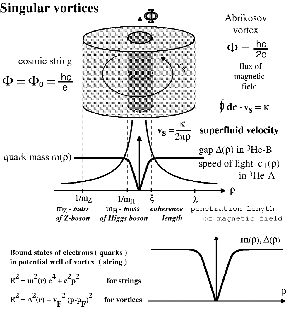
FIG. 14.: Singular vortex and cosmic string. top: Abrikosov vortex in superconductor is analog of the Nielsen-Olesen cosmic string. The role of the penetration length $\lambda$ is played by the inverse mass of the $Z$-boson. If $\lambda\gg\xi$, the core size, within the region of dimension $\lambda$ the Abrikosov vortex has the same structure as the vortex in neutral superfluids, such as ³He-B, where the circulation of the superfluid velocity is quantized. bottom: Masses of quarks and the gap of qusiparticles in superconductors are suppressed in the vortex core. The core serves as potential well for fermions which are bound in the vortex forming fermion zero modes.

The process of the momentum generation by vortex cores is similar to that of generation of baryonic by the cores of cosmic strings [113, 114, 115, 116, 117]. The axial anomaly is instrumental for the baryoproduction in the core of cosmic strings, but again the effect cannot be described by the anomaly equation (130), which was derived using the energy spectrum of the free massless fermions in the presence of the homogeneous electric and magnetic fields. But in cosmic strings these fields are no more homogeneous. Moreover the massless fermions exist only in the vortex core as bound states in the potential well produced by the order parameter (Higgs) field. Thus the consideration of baryoproduction by cosmic strings and momentogenesis by singular vortices should be studied using the spectrum of the massless (or almost massless) bound states, the fermion zero modes.

A Fermion zero modes on vortices

1 Anomalous branch of chiral fermions

The spectrum of the low-energy bound states in the core of the axisymmetric vortex with winding number $n_{1}=\pm 1$ in the isotropic model of $s$-wave superconductor was obtained in microscopic theory by Caroli, de Gennes and Matricon [118]:

$$E(L_{z})=-n_{1}\omega_{0}L_{z}~{}.$$ (192)

This spectrum is two-fold degenerate due to spin degrees of freedom; $L_{z}$ is the generalized angular momentum of the fermions in the core, which was found to be half of odd integer quantum number (Fig. 15). The level spacing $\omega_{0}$ is small compared to the energy gap of the quasiparticles outside the core, $\omega_{0}\sim\Delta_{0}^{2}/E_{F}\ll\Delta_{0}$. This level spacing $\omega_{0}$ is called the minigap, because $\omega_{0}/2$ is the minimal energy of quasiparticle in the core. In the 3D systems the minigap depends on the momentum $p_{z}$ along the vortex line. Here for simplicity we shall consider the 2D case, when the vortex lines are reduced to point vortices.

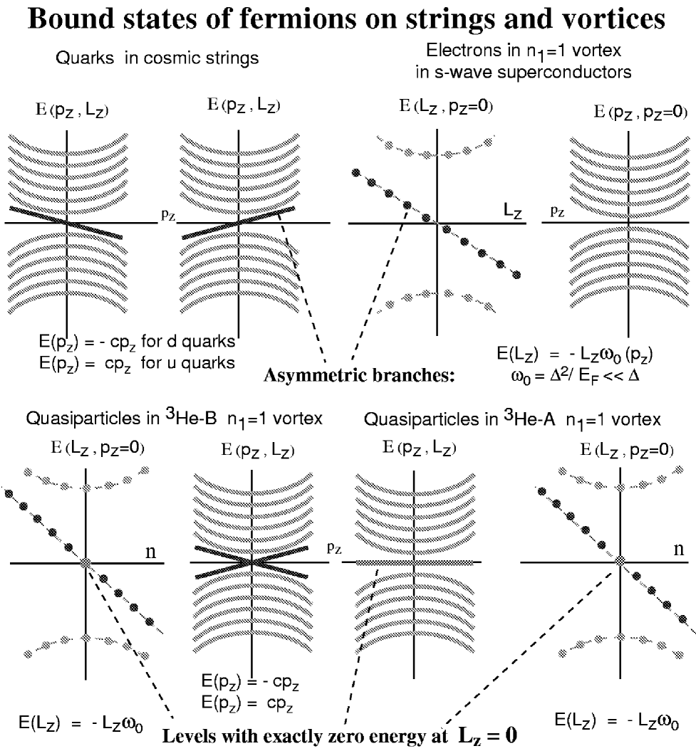
FIG. 15.: Fermion zero modes on strings and on different condensed matter vortices.

Since the minigap is small, in many physical cases the discreteness of $L_{z}$ can be neglected and in quasiclassical approximation one can consider this quantum number as continuous. Then from Eq.(192) it follows that the spectrum as a function of continuous angular momentum $L_{z}$ contains an anomalous branch, which crosses zero energy (Fig. 15). Thus in the quasiclasical approximation one has fermion zero modes on vortices. The fermions in this 1D “Fermi liquid” are chiral: the positive energy fermions have a definite sign of the angular momentum $L_{z}$. In general case of arbitrary winding number $n_{1}$, the number of fermion zero modes, i.e. the number of branches crossing zero level as a function of $L_{z}$, equals $-2n_{1}$ (see Ref.[90]). This represents an analogue of the index theorem known for cosmic strings in the relativistic quantum field theory (see Ref.[119] and references therein). The difference is that in strings the spectrum of relativistic fermions crosses zero energy as a function of $p_{z}$ (Fig. 15). As a result the index theorem discriminates between left-moving and right-moving fermions, while in condensed matter vortices the index theorem discriminates between cw and ccw rotating fermions.

2 Integer vs half-odd-integer angular momentum of fermion zero modes

The above properties of the fermions bound to the vortex core are universal and do not depend on the detailed structure of the vortex core. If we now proceed to the non-$s$-wave superfluid or superconducting states, we find that the situation does not change, with one exception: in some vortices the quantum number $L_{z}$ is half of odd integer, in the others it is integer. In the vortices of second type there is a true zero mode: at $L_{z}=0$ the quasiparticle energy in Eq.(192) is exactly zero. This true zero-energy bound state was first calculated in a microscopic theory [120] for the $n_{1}=\pm 1$ vortex in ³He-A. This difference between two types of the fermionic spectrum becomes important at low temperature $T<\omega_{0}$.

We consider here the representatives of these two types of vortices: the traditional $n_{1}=\pm 1$ vortex in $s$-wave superconductor (Fig. 15 top right) and the simplest form of the $n_{1}=\pm 1$ vortex in ³He-A with $\hat{\bf l}$ directed along the vortex axis (Fig. 15 bottom right). Their order parameters are

$$\Psi({\bf r})=\Delta_{0}(\rho)e^{in_{1}\phi}~{},~{}~{}\oint d{\bf x}\cdot{\bf v}_{\rm s}=n_{1}\pi\hbar/m~{},$$ (193)

$$A_{\mu\,i}=\Delta_{0}(\rho)e^{in_{1}\phi}\hat{z}_{\mu}\left(\hat{x}_{i}+i\hat{y}_{i}\right)~{},~{}~{}\oint d{\bf x}\cdot{\bf v}_{\rm s}=n_{1}\pi\hbar/m~{},$$ (194)

where $z$, $\rho$, $\phi$ are the coordinates of the cylindrical system with the axis $z$ along the vortex line; and $\Delta_{0}(\rho)$ is the profile of the order parameter amplitude in the vortex core with $\Delta_{0}(\rho=0)=0$. The structure of the spectrum of the fermion zero modes does nor depend on the profile of $\Delta_{0}(\rho)$.

3 Hamiltonian for fermions in the core

After diagonalization over spin indices one finds that for each of two spin components the Bogoliubov – Nambu Hamiltonian for quasiparticles in the presence of the vortex has the form

$${\cal H}=\left(\matrix{M(p)&\Delta_{0}(\rho)e^{in_{1}\phi}\left({p_{x}+ip_{y}\over p_{F}}\right)^{N_{3}}\cr\Delta_{0}(\rho)e^{-in_{1}\phi}\left({p_{x}-ip_{y}\over p_{F}}\right)^{N_{3}}&-M(p)\cr}\right)~{}.$$ (195)

Here the integer index $N_{3}=0$ for the case of vortex in $s$-wave superfluid in Eq.(193) and $N_{3}=1$ for the ³He-A case ( Eq.(194)). For simplicity we assumed the 2D spatial dimension, which is applicable for thin superfluid/superconducting films. In general 2D system the integral index $N_{3}$ is the topological invariant in the momentum space, Eq.(71), which is responsible for the Chern – Simons terms in the 2D superfluids/superconductors [41, 42, 44]. The two types of the fermion zero modes, which we discuss, are determined by the parity $W=(-1)^{n_{1}+N_{3}}$, which is constructed from the topological charges in real and momentum spaces [121].

In what follows the fast radial motion of the fermions in the vortex core is integrated out to obtain only the slow motion corresponding to the low-energy fermion zero modes on anomalous branch. It is important that the characteristic size $\xi$ of the vortex core is much larger than the wave length $\lambda=2\pi/p_{F}$ of quasiparticle: $\xi p_{F}\sim E_{F}/\Delta_{0}\sim c_{\parallel}/c_{\perp}\sim 10^{3}$. Thus for the radial motion we can use the quasiclassical description in terms of trajectories, which are almost the straight lines crossing the core. The description in terms of the trajectories are valid in the quasiclassical region of energies between the two “Planck” scales, $\omega_{0}\sim\Delta_{0}^{2}/v_{F}p_{F}\ll E\ll\Delta_{0}$ discussed in Sec. V A 4.

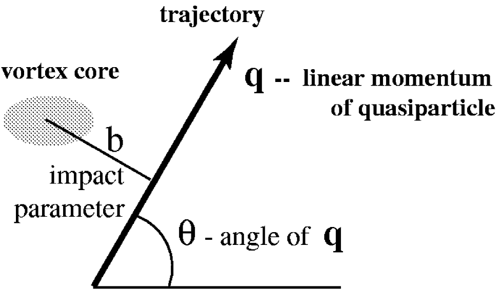
FIG. 16.: In the quasiclassical approximation trajectories of quasiparticle are straight lines.

The low energy trajectories through the vortex core are characterized by the direction $\theta$ of the trajectory and the impact parameter $b$ (Fig. 16). The magnitude of the momentum of quasiparticle along trajectory is close to $p_{F}$, so that the momentum ${\bf p}$ is close to the value

$${\bf q}=p_{F}(\hat{\bf x}\cos\theta+\hat{\bf y}\sin\theta)~{},$$ (196)

and the velocity is close to ${\bf v}_{F}={\bf q}/m^{*}$. In terms of the angle $\theta$ the Eq.(195) can be rewritten in the form

$${\cal H}=\left(\matrix{M(p)&\Delta_{0}(\rho)e^{i(n_{1}\phi+N_{3}\theta)}\cr\Delta_{0}(\rho)e^{-i(n_{1}\phi+N_{3}\theta)}&-M(p)\cr}\right)~{},$$ (197)

which emphasizes the interplay between the real-space and momentum-space topologies.

Substituting $\chi\rightarrow e^{i{\bf q}\cdot{\bf r}}\chi$ and ${\bf p}\rightarrow{\bf q}-i{\bf\nabla}$, and expanding in small ${\bf\nabla}$, one obtains the quasiclassical Hamiltonian for the fixed trajectory $({\bf q},b)$:

$${\cal H}_{{\bf q},b}=-i\check{\tau}_{3}{\bf v}_{F}\cdot{\bf\nabla}+\Delta_{0}(\rho)\left(\check{\tau}_{1}\cos(N_{3}\theta+n_{1}\phi)-\check{\tau}_{2}\sin(N_{3}\theta+n_{1}\phi)\right)~{}.$$ (198)

Since the coordinates $\rho$ and $\phi$ are related by equation $\rho\sin(\phi-\theta)=b$, the only argument is the coordinate along the trajectory $s=\rho\cos(\phi-\theta)$ and thus the Hamiltonian in Eq.(198) has the form

$${\cal H}_{{\bf q},b}=-i{v}_{F}\check{\tau}_{3}\partial_{s}+\check{\tau}_{1}\Delta_{0}(\rho)\cos\left(n_{1}\tilde{\phi}+(n_{1}+N_{3})\theta\right)-$$ (199)

$$-\check{\tau}_{2}\Delta_{0}(\rho)\sin\left(n_{1}\tilde{\phi}+(n_{1}+N_{3})\theta\right)~{},$$ (200)

where $\tilde{\phi}=\phi-\theta$ is expressed in terms of the coordinate $s$ as

$$\tilde{\phi}=\phi-\theta~{}~{},~{}~{}\tan\tilde{\phi}={b\over s}~{}~{}.$$ (201)

The dependence of the Hamiltonian on the direction $\theta$ of the trajectory can be removed by the following transformation:

$$\chi=e^{i(n_{1}+N_{3})\check{\tau}_{3}\theta/2}\tilde{\chi},$$ (202)

$$\tilde{\cal H}_{{\bf q},b}=e^{-i(n_{1}+N_{3})\check{\tau}_{3}\theta/2}{\cal H}e^{i(n_{1}+N_{3})\check{\tau}_{3}\theta/2}=$$ (203)

$$=-i{v}_{F}\check{\tau}_{3}\partial_{s}+\Delta_{0}(\sqrt{s^{2}+b^{2}})\left(\check{\tau}_{1}\cos n_{1}\tilde{\phi}-\check{\tau}_{2}\sin n_{1}\tilde{\phi}\right)~{}.$$ (204)

The Hamiltonian in Eq.(204) does not depend on the angle $\theta$ and on the topological charge $N_{3}$ and thus is the same for $s$, $p$ and other pairing states. The dependence on $N_{3}$ enters only the boundary condition for the wave function, which according to Eq.(202) is

$$\tilde{\chi}(\theta+2\pi)=(-1)^{n_{1}+N_{3}}\tilde{\chi}(\theta)$$ (205)

With respect to this boundary condition, there are two classes of systems: with odd and even $n_{1}+N_{3}$. The parity $W=(-1)^{n_{1}+N_{3}}$ thus determines the spectrum of fermions in the vortex core.

4 Quasiclassical low-energy states on anomalous branch

The state with the lowest energy corresponds to trajectories, which cross the center of the vortex, i.e. with $b=0$. Along this trajectory one has $\sin\tilde{\phi}=0$ and $\cos\tilde{\phi}={\rm sign}~{}s$. So that the Eq.(204) becomes

$$\tilde{\cal H}_{{\bf q},b}=-i{v}_{F}\check{\tau}_{3}\partial_{s}+\check{\tau}_{1}\Delta_{0}(|s|){\rm sign}~{}s~{}.$$ (206)

It is supersymmetric and thus contains the eigenstate with zero energy. Let us write the corresponding eigen function including all the transformations:

$$\chi_{\theta,b=0}(s)=e^{ip_{F}s}e^{i(n_{1}+N_{3})\check{\tau}_{3}\theta/2}\left(\matrix{1\cr-i\cr}\right)\chi_{0}(s)~{}~{},$$ (207)

$$\chi_{0}(s)=\exp{\left(-\int^{s}ds^{\prime}{\rm sign}~{}s^{\prime}{\Delta_{0}(|s^{\prime}|)\over v_{F}}\right)}~{}.$$ (208)

Now we can consider the case of nonzero impact parameter. When $b$ is small the third term in Eq.(204) can be considered as perturbation and its average over the wave function in Eq.(207) gives the energy levels in terms of $b$ and thus in terms of the continuous angular momentum $L_{z}=p_{F}b$:

$$E(L_{z},\theta)=-n_{1}L_{z}\omega_{0}~{},~{}\omega_{0}={\int_{0}^{\infty}d\rho{\Delta_{0}(\rho)\over p_{F}\rho}\exp{\left(-{2\over v_{F}}\int_{0}^{\rho}d\rho^{\prime}\Delta_{0}(\rho^{\prime})\right)}\over\int_{0}^{\infty}d\rho\exp{\left(-{2\over v_{F}}\int_{0}^{\rho}d\rho^{\prime}\Delta_{0}(\rho^{\prime})\right)}}~{}.$$ (209)

This is the anomalous branch of chiral fermions which crosses zero energy in semiclassical approximation, when $L_{z}$ is continuous variable. For nonaxisymmetric vortices the quasclassical energy depends also on $\theta$. The minigap $\omega_{0}$ is of order $\omega_{0}\sim\Delta_{0}/(p_{F}R)$ where $R$ is the radius of core. Typically $i$ is of order coherence length $\xi=v_{F}/\Delta_{0}$ and the minigap is $\omega_{0}\sim\Delta_{0}^{2}/(p_{F}v_{F})\ll\Delta_{0}$. In a large temperature region $\Delta_{0}^{2}/(p_{F}v_{F})<T<\Delta_{0}$ these bound fermionc states can be considered as fermion zero modes.

5 Quantum low-energy states and $W$-parity.

In exact quantum mechanical problem the generalized angular momentum $L_{z}$ has discrete eigen values. To find quantized energy levels we take into account that the two remaining degrees of freedom, the angle $\theta$ and the momentum $L_{z}$, are canonically conjugated variables [122, 123]. That is why the next step is the quantization of motion in the $\theta,L_{z}$ plane which can be obtained from the quasiclassical energy in Eq.(209), if $L_{z}$ is considered as an operator. For the axisymmetric vortex, the Hamiltonian does not depend on $\theta$

$$H=in_{1}\omega_{0}\partial_{\theta}$$ (210)

and has the eigenfunctions $e^{-iE\theta/n_{1}\omega_{0}}$. The boundary condition for these functions, the Eq.(205), gives the quantized energy levels, which depend on the $W$-parity:

$$E(L_{z})=-n_{1}L_{z}\omega_{0}~{},$$ (211)

$$L_{z}=n~{}~{},~{}~{}W=+1~{}~{};$$ (212)

$$L_{z}=\left(n+{1\over 2}\right)~{}~{},~{}~{}W=-1~{}~{},$$ (213)

where $n$ is integer.

The phase $(n_{1}+N_{3})\tau_{3}\theta/2$ in Eq.(202) plays the part of Berry phase. It shows how the wave function of quasiparticle changes, when the trajectory is adiabatically rotating by angle $\theta$. This Berry phase is instrumental for the Bohr – Sommerfeld quantization of the energy levels in the vortex core. It chooses between the only two possible quantizations consistent with the “CPT-symmetry” of states in superconductors: $E=n\omega_{0}$ and $E=(n+1/2)\omega_{0}$. In both cases for each positive energy level $E$ one can find another level with the energy $-E$. That is why the above quantization is applicable even to nonaxisymmetric vortices, though the quantum number $L_{z}$ is no more the angular momentum there.

Fig. 15 shows the quasiparticle spectrum in the core of vortex lines in 3D space. In the top-right corner it is the spectrum in the core of vortices with $W=-1$. At the bottom the spectrum of bound states in the core of vortices with $W=1$ is shown. These are the real fermion zero modes, since they cross zero energy. The most interesting situation occurs for the ³He-A vortices which contains a self conjugated zero-energy level. This $E=0$ level is doubly degenerate due to spin. Such exact zero mode is robust to any deformations, which preserve the spin degeneracy. This is the reason why the branch with $L_{z}=0$ has zero energy for all momenta $p_{z}$ (right bottom corner of Fig. 15) as was first found in microscopic theory by Kopnin [120] (see also [121]).

6 Majorana fermion with $E=0$ on half-quantum vortex.

The most exotic situation will occur for the half-quantum vortex [124], which can exist in thin ³He-A films or in layered chiral superconductors with the same order parameter. The order parameter in Eq.(85) outside the core of $n_{1}=1/2$-vortex is

$$A_{\mu\,i}=\Delta_{0}\hat{d}_{\mu}\left(\hat{e}_{1i}+i\hat{e}_{2i}\right)=\Delta_{0}\left(\hat{x}_{\mu}\cos{\phi\over 2}+\hat{y}_{\mu}\sin{\phi\over 2}\right)\left(\hat{x}_{i}+i\hat{y}_{i}\right)e^{i\phi/2}~{}.$$ (214)

The change of the sign of the vector $\hat{\bf d}$ when circumscribing around the core is compensated by the change of the phase of the order parameter by $\pi$ at which the sign of the exponent $e^{i\phi/2}$ also changes. Thus the whole order parameter is smoothly connected after circumnavigating. Because of the $\pi$ change of the phase around the vortex, the circulation of the superfluid velocity around the vortex $\oint d{\bf x}\cdot{\bf v}_{\rm s}=n_{1}\pi\hbar/m$ corresponds to $n_{1}=1/2$. That is why the name half-quantum vortex. This vortex still had not been observed in ³He-A but its discussion has been extended to the flux quantization with the half of conventional magnitude in superconductors [125], which finally led to the observation of the fractional flux in high-temperature superconductors: the $n_{1}=1/2$ vortex is attached to the tricrystal line, which is the junction of three grain boundaries [126].

For quasiparticles in the core of the $n_{1}=1/2$ vortex, after spin diagonalization one obtains the Hamiltonian in Eq.(197), where for one of the spin components one has $n_{1}=1$, while for the other component $n_{1}=0$. The $E=0$ level occurs only for one spin component. Since it is the only level with $E=0$ it cannot be moved from the $E=0$ position by any perturbation: its shift is prohibited by the “CPT”-symmetry.

There are many interesting properties related to this $E=0$ level. Since the $E=0$ level can be either filled or empty, there is a fractional entropy $(1/2)ln~{}2$ per layer per vortex. The factor (1/2) appears because in the pair correlated superfluids/superconductors one must take into account that we artificially doubled the number of fermions introducing both the particles and holes. On the $E=0$ level the particle excitation coincides with its antiparticle (hole), i.e. the quasiparticle is a Majorana fermion [127]. Majorana fermions at $E=0$ level lead to the non-Abelian statistics of half-quantum vortices: the interchange of two point vortices becomes identical operation (up to an overall phase) only on being repeated four times [112]. This can be used for quantum computing [128].

7 Fermions on asymmetric vortices.

Most of vortices in condensed matter are not axisymmetric. In superconductors the rotational symmetry is violated by crystal lattice, while in superflud ³He the axisymmetry is as a rule spontaneously broken in the core or outside the core (see e.g. [129]). The general form of the $a$-th branch of the low-energy spectrum of fermions, which cross zero in quasiclassical approximation is (see [123])

$$E_{a}(L_{z},\theta)=\omega_{a}(\theta)(L_{z}-L_{za}(\theta))$$ (215)

For given $\theta$ the spectrum crosses zero energy at some $L_{z}=L_{za}(\theta)$. The ”CPT”-symmetry of the Bogoliubov-Nambu Hamiltonian requires that if $E_{a}(L_{z}Q,\theta)$ is the energy of the bound state fermion, then $-E_{a}(-L_{z},\theta+\pi)$ also corresponds to the energy of quasiparticle in the core.

Let us consider one pair of the conjugated branches related by the “CPT” symmetry. One can introduce the common gauge field $A_{\theta}(\theta,t)$ and the ”electric” charge $e=\pm 1$, so that $Q_{\pm}=eA_{\theta}$. Then the quantum Hamiltonian becomes

$${\cal H}=-{n_{1}\over 2}\left\{~{}\omega_{0}(\theta)~{},~{}\sum_{e}\left(-i{\partial\over\partial\theta}-eA_{\theta}(\theta,t)\right)\right\}~{}~{},$$ (216)

where $\{~{},~{}\}$ is anticommutator. The Schrödinger equation for the fermions on the $a$-th branch is

$${i\over 2}(\partial_{\theta}\omega_{0})\Psi(\theta)+\omega_{0}(\theta)\left(i\partial_{\theta}+eA(\theta)\right)\Psi(\theta)=n_{1}E\Psi(\theta)$$ (217)

The normalized eigen functions are

$$\Psi(\theta)=\left<{1\over\omega_{0}(\theta)}\right>^{-1/2}~{}{1\over\sqrt{2\pi\omega_{0}(\theta)}}\exp\left(i\int^{\theta}d\theta^{\prime}\left({n_{1}E\over\omega_{0}(\theta^{\prime})}+eA(\theta^{\prime})\right)\right)~{}~{}.$$ (218)

Here the angular brackets mean the averaging over the angle $\theta$.

For the self-conjugated branch according to the “CPT”-theorem one has $\int^{2\pi}_{0}d\theta A(\theta)=0$, then using the boundary conditions in Eq.(205) one obtains the equidistant energy levels:

$$E_{n}=\left(n+{1-W\over 4}\right)\left<{1\over\omega_{0}(\theta)}\right>^{-1}~{}~{}.$$ (219)

For axisymmetric vortices the integral index $n$ is determined by the azimuthal quantum number $L_{z}$. For the nonaxisymmetric vortex, $L_{z}$ is not a good quantum number. Nevertheless the properties of the anomalous branch of fermion modes on vortices are not disturbed by the nonaxisymmetric perturbations of the vortex core structure, which lead only to the renormalization of the minigap. These properties are dictated by real- and momentum-space topology and are robust to perturbations.

B Spectral flow in singular vortices: Callan-Harvey mechanism of anomaly cancellation

Now let us consider again the force, which arise when the vortex moves with respect to the heat bath. In Sec. VII D we discussed this for the special case of the continuous ³He-A vortex texture where the macroscopic Adler-Bell-Jackiw anomaly equation could be used. Now we consider this effect using the microscopic description of the spectral flow of fermion zero modes within the vortex core. We show that the same force arises for any vortex in any superfluid or superconductor under a special condition.

If the vortex moves with the velocity ${\bf v}_{L}$ with respect to the heat bath, the coordinate ${\bf r}$ is replaced by the ${\bf r}-{\bf v}_{L}t$. The angular momentum $L_{z}$, which enters the quasiclassical energy of quasiparticle in Eq.(209), shifts with time, because the momentum is ${\bf r}\times{\bf p}$. So the energy becomes

$$E(L_{z},\theta)=-n_{1}\left(L_{z}-\hat{\bf z}\cdot({\bf v}_{L}\times{\bf q})t\right)\omega_{0}~{}.$$ (220)

Here $E_{z}=\hat{\bf z}\cdot({\bf v}_{L}\times{\bf q})$ acts on fermions localized in the core in the same way that an electric field $E_{z}$ acts on chiral fermions on an anomalous branch in magnetic field or the chiral fermion zero modes localized on a string in relativistic quantum theory. The only difference is that under this “electric” field the spectral flow in the vortex occurs in the $L_{z}$ direction (${\dot{L}}_{z}=eE_{z}$) rather than along $p_{z}$ direction in strings where ${\dot{p}}_{z}=eE_{z}$. Since according to index theorem, for each quantum number $L_{z}$ there are $-2n_{1}$ quasiparticle levels, the fermionic levels cross the zero energy at the rate

$${\dot{n}}=-2n_{1}{\dot{L}}_{z}=-2n_{1}E_{z}({\bf q})=-2n_{1}\hat{\bf z}\cdot({\bf v}_{L}\times{\bf q})~{}~{}.$$ (221)

When the occupied level crosses zero, the quasiparticle on this level transfers its fermionic charges from the vacuum (from the negative energy states) along the anomalous branch into the heat bath (“matter”). For us the important fermionic charge is linear momentum. The rate at which the momentum ${\bf q}$ is transferred from the vortex to the heat bath due to spectral flow

$$\partial_{t}{\bf P}={1\over 2}\int_{0}^{2\pi}{{d\theta}\over{2\pi}}~{}{\bf q}\dot{n}=$$ (222)

$$-n_{1}\int_{0}^{2\pi}{{d\theta}\over{2\pi}}~{}{\bf q}\left(\hat{\bf z}\cdot(({\bf v}_{L}-{\bf v}_{\rm n})\times{\bf q})\right)=-n_{1}{{p_{F}^{2}}\over 2}\hat{\bf z}\times({\bf v}_{L}-{\bf v}_{\rm n})~{}~{}.$$ (223)

The factor $1/2$ in Eq.(222) is to compensate the double counting of particles and holes.

The extension to the 3+1 case is straightforward. The trajectory in the plane perpendicular to the vortex axis is now characterized by the transverse momentum

$${\bf q}=\sqrt{p_{F}^{2}-p_{z}^{2}}~{}(\hat{\bf x}\cos\theta+\hat{\bf y}\sin\theta)~{},$$ (224)

so that the total momentum is on the Fermi surface: ${\bf q}^{2}+p_{z}^{2}=p_{F}^{2}$. Due to that the momentum production is slightly modified:

$$\partial_{t}{\bf P}={1\over 2}\int_{0}^{2\pi}{{d\theta}\over{2\pi}}\int_{-p_{F}}^{p_{F}}{{dp_{z}}\over{2\pi}}~{}{\bf q}\dot{n}=$$ (225)

$$-n_{1}\int_{-p_{F}}^{p_{F}}{{dp_{z}}\over{2\pi}}(p_{F}^{2}-p_{z}^{2})\int_{0}^{2\pi}{{d\theta}\over{2\pi}}~{}\hat{\bf q}\left(\hat{\bf z}\cdot(({\bf v}_{L}-{\bf v}_{\rm n})\times\hat{\bf q})\right)=$$ (226)

$$-n_{1}{{p_{F}^{3}}\over 3\pi}\hat{\bf z}\times({\bf v}_{L}-{\bf v}_{\rm n})~{}~{}.$$ (227)

Thus the spectral flow force acting on a vortex from the system of quasiparticles is

$${\bf F}_{sf}=-\pi n_{1}\hbar C_{0}{\hat{\bf z}}\times({\bf v}_{\rm L}-{\bf v}_{\rm n}).$$ (228)

This is in agreement with the result in Eq.(142) obtained for the $n_{1}=2$ continuous vortex using the Adler-Bell-Jackiw equation. We recall that the parameter of the axial anomaly is $C_{0}=p_{F}^{3}/3\pi^{2}$ in 3D, while in 2D case it is $C_{0}=p_{F}^{2}/2\pi$ in agreement with Eq.(223).

In this derivation it was implied that all the quasiparticles, created from the negative levels of the vacuum state, finally become part of the normal component, i.e. there is a nearly reversible transfer of linear momentum from fermions to the heat bath. This should be valid in the limit of large scattering rate: $\omega_{0}\tau\ll 1$, where $\tau$ is the lifetime of the fermion on the $L_{z}$ level. This condition, which states that the interlevel distance on the anomalous branch is small compared to the life time of the level, is the crucial requirement for spectral flow to exist. In the opposite limit $\omega_{0}\tau\gg 1$ the spectral flow is suppressed and the corresponding spectral flow force is exponentially small [123] (see Sec. IX B 1 below). This shows the limitation for exploring the macroscopic Adler-Bell-Jackiw anomaly equation in the electroweak model and in ³He-A.

The process of transfer of linear momentum from the superfluid vacuum to the normal motion of fermions within the core is the realization of the Callan-Harvey mechanism for anomaly cancellation [89]. In the case of the condensed matter vortices the anomalous nonconservation of linear momentum in the 1+1 world of the vortex core fermions and the anomalous nonconservation of momentum in the 3+1 world outside the vortex core compensate each other. This is the same kind of the Callan-Harvey effect which has been discussed in Sec. VII D for the motion of continuous textures in ³He-A. As distinct from ³He-A, where there are gap nodes and chiral anomaly, the Callan-Harvey effect for singular vortices occurs in any Fermi-superfluid: the anomalous fermionic $L_{z}$ branch, which mediates the momentum exchange, exists in any topologically nontrivial singular vortex: the chirality of fermions and the anomaly are produced by the notnrivial topology of the vortex. In the limit $\omega_{0}\tau\ll 1$ this type of Callan-Harvey effect does not depend on the detailed structure of the vortex core and even on the type of pairing, and is determined solely by the vortex winding number $n_{1}$ and anomaly parameter $C_{0}$.

The first derivation of the spectral-flow force acting on a vortex was made by Kopnin and Kravtsov in Ref. [130] who used the fully microcopic BCS theory in Gor’kov formulation. It was developed further by Kopnin and coauthors. That is why it is sometimes called the Kopnin force.

1 Restricted spectral flow in the vortex core.

The semiclassical approach allows us to extend the derivation of the spectral flow dynamics to the more complicated cases, when for example the core is not symmetric or when the relation $\omega_{0}\tau\ll 1$ is not fulfilled and the spectral flow is partially suppressed. Since the spectral flow occurs through the zero energy, it is fully determined by the low-energy spectrum. As in the cases of the universality classes in the 3+1 system, the 1+1 systems also have universality classes which determine the quasiparticle spectrum in the low energy corner. In our case the generic spectrum of 1+1 fermions living in the vortex core is given by Eq.(215). Note that the coordinate in the “spatial” dimension is the angle $\theta$, i.e. the effective space is circumference $U(1)$.

Let us choose the frame of the moving vortex. In this frame the energy of quasiparticle is well determined and the Hamiltonian for quasiparticles in the moving vortex is given by

$$E_{a}(L_{z},\theta)=\omega_{a}(\theta)(L_{z}-L_{za}(\theta))+({\bf v}_{\rm s}-{\bf v}_{L})\cdot{\bf q}~{},$$ (229)

where the last term comes from the Doppler shift. We again consider the vortex in the 2D case where ${\bf q}=(p_{F}\cos\theta,p_{F}\sin\theta)$. Kinetics of these low-energy quasiparticles is given by the Boltzmann equation for the distribution function $f_{a}(L_{z},\theta)$ [122]. Let us consider the simplest case of axisymmetric vortex with one anomalous branch, then $\omega_{a}(\theta)=-n_{1}\omega_{0}L_{z}$, $L_{za}(\theta)=0$, and the Boltzmann equation becomes (in $\tau$ approximation):

$$\partial_{t}f-n_{1}\omega_{0}\partial_{\theta}f-\partial_{\theta}(({\bf v}_{\rm s}-{\bf v}_{L})\cdot{\bf q})~{}\partial_{L_{z}}f=-{f(L_{z},\theta)-f_{{\cal T}}(L_{z},\theta)\over\tau}~{}.$$ (230)

The equilibrium distribution $f_{{\cal T}}$ corresponds to the state, when the vortex moves together with the heat bath, i.e. when ${\bf v}_{L}={\bf v}_{\rm n}$:

$$f_{{\cal T}}(L_{z},\theta)=\left(1+\exp{-n_{1}\omega_{0}L_{z}+({\bf v}_{\rm s}-{\bf v}_{\rm n})\cdot{\bf q}\over T}\right)^{-1}~{}.$$ (231)

When ${\bf v}_{L}\neq{\bf v}_{\rm n}$ the equilibrium is volated and the distribution function evolves according to the Eq.(230).

Introducing new variable $l=L_{z}-n_{1}({\bf v}_{\rm s}-{\bf v}_{\rm n})\cdot{\bf q}$ (we consider here $n_{1}=\pm 1$) one obtains the equation for $f(l,\theta)$ which does not contain ${\bf v}_{\rm s}$:

$$\partial_{t}f-n_{1}\omega_{0}\partial_{\theta}f-\partial_{\theta}(({\bf v}_{\rm n}-{\bf v}_{L})\cdot{\bf q})~{}\partial_{l}f=-{f(l,\theta)-f_{{\cal T}}(l)\over\tau}~{}.$$ (232)

Since we are interested in the momentum transfer only we can write equation for the net momentum of quasiparticles

$${\bf P}={1\over 2}\int dl\int{d\theta\over 2\pi}f(l,\theta){\bf q}~{},$$ (233)

which is

$$\partial_{t}{\bf P}-n_{1}\omega_{0}\hat{\bf z}\times{\bf P}+\pi C_{0}\hat{\bf z}\times({\bf v}_{\rm n}-{\bf v}_{L})(f_{{\cal T}}(\Delta_{0}(T))-f_{{\cal T}}(-\Delta_{0}(T)))=-{{\bf P}\over\tau}~{}.$$ (234)

Here we first consider only the bound states below the gap $\Delta_{0}(T)$ and thus the integral $\int dl\partial_{l}n$ is limited by $\Delta_{0}(T)$. That is why the inegral gives $f_{{\cal T}}(\Delta(T))-f_{{\cal T}}(-\Delta(T))=-\tanh(\Delta_{0}(T)/2T)$.

In the steady state of ht evortex motion one has $\partial_{t}{\bf P}=0$ and the solution for the steady state momentum can be easily found [122]. As a result one obtains the following contribution to the spectral flow force due to bound states below $\Delta_{0}(T)$:

$${\bf F}_{sf~{}bound}={{\bf P}\over\tau}=-{\pi C_{0}\over 1+\omega_{0}^{2}\tau^{2}}\tanh{\Delta_{0}(T)\over 2T}[({\bf v}_{L}-{\bf v}_{\rm n})\omega_{0}\tau+n_{1}\hat{\bf z}\times({\bf v}_{L}-{\bf v}_{\rm n})].$$ (235)

This equation contains both the nondissipative and friction forces. Now one must add the contribution of unbound states above the gap $\Delta_{0}(T)$. The spectral flow there is not suppressed, since the distance between the levels in the continuous spectrum is $\omega_{0}=0$. This gives the spectral flow contribution from the thermal tail of the continuous spectrum

$${\bf F}_{sf~{}unbound}=-\pi n_{1}C_{0}\left(1-\tanh{\Delta_{0}(T)\over 2T}\right)\hat{\bf z}\times({\bf v}_{L}-{\bf v}_{\rm n})~{}.$$ (236)

Finally the total spectral-flow force is the sum of two contributions, Eqs.(235-236). The nondissipative part of the force is

$${\bf F}_{sf}=-\pi n_{1}C_{0}\left[1-{\omega_{0}^{2}\tau^{2}\over 1+\omega_{0}^{2}\tau^{2}}\tanh{\Delta_{0}(T)\over 2T}\right]\hat{\bf z}\times({\bf v}_{L}-{\bf v}_{\rm n})~{},$$ (237)

while the contribution of the spectral flow to the friction force is

$${\bf F}_{fr}=-\pi C_{0}\tanh{\Delta_{0}(T)\over 2T}~{}{\omega_{0}\tau\over 1+\omega_{0}^{2}\tau^{2}}({\bf v}_{L}-{\bf v}_{n})~{}.$$ (238)

2 Measurement of Callan-Harvey effect in ³He-B

The equations (237) and (238) are applied for the dynamics of singular vortices in ³He-B, where the minigap $\omega_{0}$ is comparable with the inverse quasiparticle lifetime and the parameter $\omega_{0}\tau$ is regulated by temperature. Introducing again the Magnus and Iordanskii forces one obtains the following dimensionless parameters $d_{\perp}$ and $d_{\parallel}$ in Eq.(146) for the balance of forces acting on a vortex:

$$d_{\perp}={C_{0}\over n_{\rm s}}\left(1-{n\over n_{\rm s}}{\omega_{0}^{2}\tau^{2}\over 1+\omega_{0}^{2}\tau^{2}}\tanh{\Delta_{0}(T)\over 2T}\right)-{n_{\rm n}\over n_{\rm s}}~{},$$ (239)

$$d_{\parallel}={C_{0}\over n_{\rm s}}{\omega_{0}\tau\over 1+\omega_{0}^{2}\tau^{2}}\tanh{\Delta_{0}(T)\over 2T}~{}.$$ (240)

FIG. 17.: Experimental verification of Callan-Harvey and gravitational Aharonov-Bohm effects in ³He-B. Solid lines are Eqs. (239) and (240). The Callan-Harvey effect is suppressed at low $T$ but becomes maximal close to $T_{c}$, where the spectral flow transfers the fermionic charge – the momentum – from the 1+1 fermionc in the core to the 3+1 bulk superfluid. The negative value of $d_{\perp}$ at intermediate $T$ demostrates the Iordanskii force, which comes from the analog of the gravitational Aharonov-Bohm effect.

The regime of the fully developed axial anomaly occurs when $\omega_{0}\tau\ll 1$. This is realized close to $T_{c}$, since $\omega_{0}$ vanishes at $T_{c}$. In this regime $d_{\perp}=(C_{0}-n_{\rm n})/n_{\rm s}\approx(n-n_{\rm n})/n_{\rm s}=1$. At lower $T$ both $\omega_{0}$ and $\tau$ increase; at $T\rightarrow 0$ one has an opposite regime, $\omega_{0}\tau\gg 1$. The spectral flow becomes completely suppressed, anomaly disappears and one obtains $d_{\perp}=-n_{\rm n})/n_{\rm s}\rightarrow 0$. This negative contribution comes solely from the Iordanskii force. Both extreme regimes and the crossover between them at $\omega_{0}\tau\sim 1$ have been observed in experiments with ³He-B vortices [38, 88, 10] (Fig. 17). The friction force is maximal in the crosover region and disappears in the two extreme regimes. In addition the experimental observation of the negative $d_{\perp}$ at low $T$ (Fig. 17) verifies the existence of the Iordanskii force; thus the analog of the gravitational Aharonov-Bohm effect (Sec. XII) has been measured in ³He-B.

X Interface between two different vacua and vacuum pressure in superfluid ³He.

Here we proceed to the effects related to the nontrivial effective gravity of quantum vacuum in superfluid ³He-A. The main source of such metric are the topological objects: (1) disgyration whose effective metric is analogous to that of the cosmic string with the large mass; (ii) quantized vortices which reproduce the effective metric of spinning cosmic string; (iii) solitons and interfaces which simulate the degenerate metric and event horizon; etc. Let us start with the interface between ³He-A and ³He-B, which appears to be useful for the consideration of the vacuum energy of states with different broken symmetry. We start with the interface between different vacua (Fig. 18).

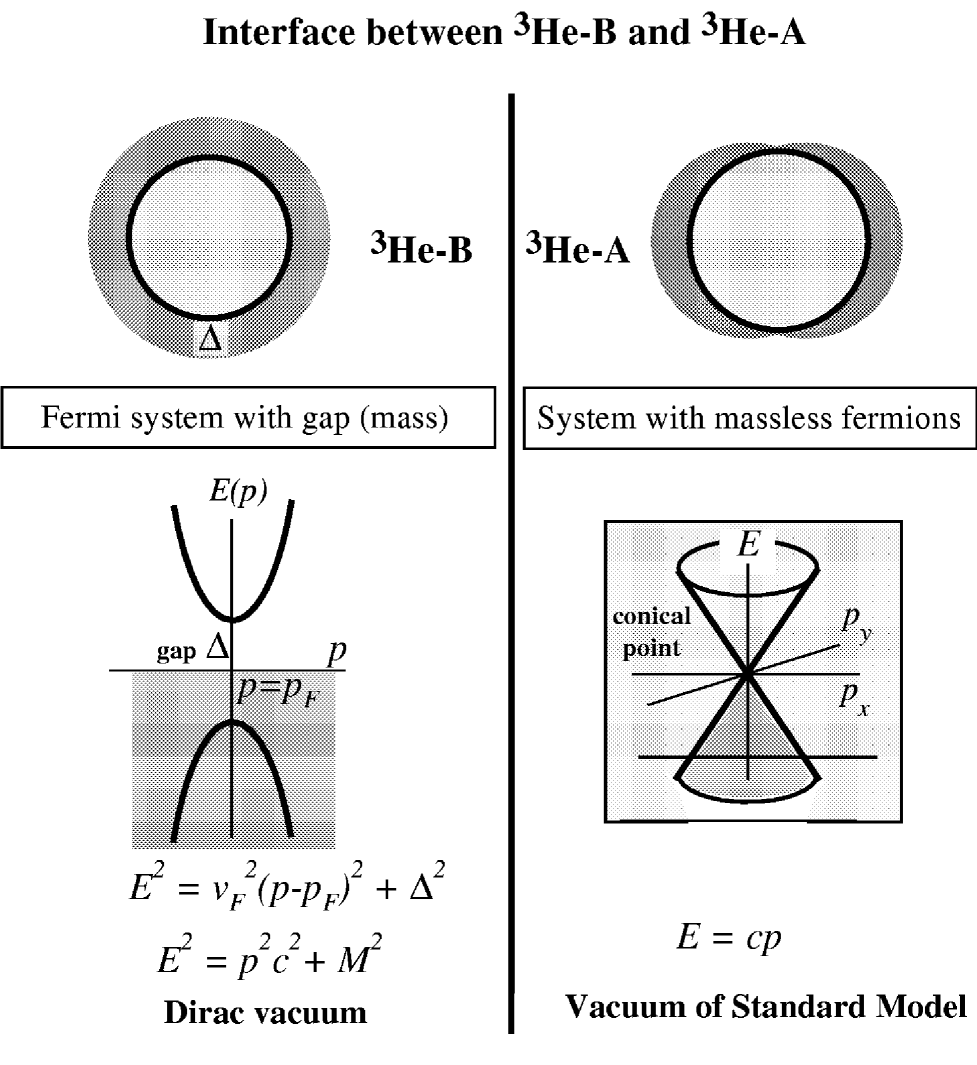
FIG. 18.: Interface between two vacua of different universality classes. Interface between ³He-A and ³He-B corresponds to the interface between the vacuum of Standard Model and vacuum of Dirac fermions. Since the low-energy (quasi)-particles cannot penetrate from the right vacuum to the left one, the interface is a perfect mirror.

A Interface between vacua of different universality classes and Andreev reflection.

1 Fermions in two neighboring vacua.

The vacua in ³He-A and ³He-B have different broken symmetries, neither of them is the subgroup of the other, [13] (Sec. V A 2). Thus the phase transition between the two superfluids is of first order. The interface between them (the AB interface) is stable and is stationary if the two phases have the same vacuum energy. The difference between energies of ³He-A and ³He-B is regulated by the magnetic field (see below) and temperature. At $T\neq 0$ the equilibrium and also the dynamics of the interface is determined by the fermionic quasiparticles (Bogoliubov excitations). In the ³He-A vacuum the fermions are chiral and massless, while in the ³He-B vacuum they are massive according to Eq.(95). At the temperature $T$ well below the temperature $T_{c}$ of the superfluid transition, when $T\ll\Delta_{0}$, the thermal fermions are present only in the ³He-A. Close to the gap nodes, i.e. at ${\bf p}\approx\pm p_{F}\hat{\bf l}$, the energy spectrum of the gapless ³He-A fermions becomes “relativistic”. Since the ³He-B excitations are massive (gapped), the thermal excitations cannot propagate from ³He-A through the AB interface (Fig. 18). The scattering of the ³He-A fermions from the interface, which in the BCS systems is known as Andreev reflection [131], is the dominating mechanism of the force experienced by the moving AB interface. Due to the relativistic character of the ³He-A fermions the dynamics of the interface becomes very similar to the motion of the perfectly reflecting mirror in relativistic theories, which was heavily discussed in the relation to the dynamic Casimir effect (see eg [132, 133, 134]). So the investigation of the interface dynamics at $T\ll T_{c}$ will give the possiblitity of the modelling of the effects of quantum vacuum. On the other hand, using the relativistic invariance one can easily calculate the forces acting on moving interface from the ³He-A heat bath in the limit of low $T$ or from the ³He-A vacuum at $T=0$. This can be done for any velocity of wall with respect to the superfluid vacuum and to the heat bath. We discuss here the velocities below the “speed of light” in ³He-A.

2 Andreev reflection at the interface.

The motion of the AB interface in the so called ballistic regime for the quasiparticles has been considered in [135, 136, 137] (see also [138]). In this regime the force on the interface comes from the mirror reflection at the interface (Andreev reflection) of the ballistically moving thermally distributed Fermi particles. As in the case of moving vortex, three velocities are of importance in this process: superfluid velocity of the vacuum ${\bf v}_{\rm s}$, normal velocity of the heat bath (“matter”) ${\bf v}_{\rm n}$ and the velocity of the interface ${\bf v}_{\rm L}$. The dissipation and thus the friction part of the force is absent when the wall is stationary in the heat bath frame, i.e. when ${\bf v}_{\rm L}={\bf v}_{\rm n}$.

Let us first recall the difference between the conventional and Andreev reflection in superfluid ³He-A. For the low-energy quasiparticles their momentum is concentrated in the vicinity of the Fermi momentum, ${\bf P}_{a}\approx-C_{a}p_{F}\hat{\bf l}$. In the conventional reflection the quasiparticle momentum is reversed, which in ³He-A means that the quasiparticle acquires an opposite chirality $C_{a}$. The momentum transfer in this process is $\Delta{\bf p}=2p_{F}\hat{\bf l}$, whose magnitude $2p_{F}$ is well above the “Planck” momentum $m^{*}c_{\perp}$. The probability of such process is exponentially small and becomes essential only if the scattering center has an atomic size $a\sim 1/p_{F}$. Such atomic-size centers are absent in the long wave limit of the effective theory. Even the AB interface cannot produce such a process since the thickness $d$ of the interface is about the coherence length $d\sim\xi=\hbar v_{F}/\Delta_{0}=(c_{\parallel}/c_{\perp})\hbar/p_{F}\sim 10^{3}~{}\hbar/p_{F}$, as a result the usual scattering from the AB interface is suppressed by huge factor $\exp(-p_{F}d/\hbar)\sim\exp(-c_{\parallel}/c_{\perp})$. Thus the nonconservation of chirality of massless chiral quasiparticle is possible, due to the “transPlanckian” physics, but it is exponentially suppressed. In relativistic theories such nonconservation of chirality occurs in the lattice models, where the distance between the Fermi points of opposite chiralities is of order of Planck momentum [39].

In Andreev reflection, instead of the momentum itself, the deviation of the momentum from the Fermi point changes sign, ${\bf p}-{\bf P}_{a}\rightarrow-({\bf p}-{\bf P}_{a})$. The velocity of quasiparticle is reversed in this process, but the momentum change can be arbitrary small, so that there is no exponential suppression. In this process the chirality $C_{a}$ of quasiparticle does not change. While in terms of the condensed matter observables, the Andreev reflection is accompanied by the transformation of the particle to the hole, it corresponds to the conventional reflection in relativistic theories.

We use the reference frame in which the interface is stationary and is situated at the plane $x=0$. In this frame the order parameter (and thus the metric) is time-independent and the energy of quasiparticles is well defined. Let us first consider the simplified version when the quasiparticles at $x>0$, where they are massless (Fig. 18), have an isotropic “relativistic” spectrum $E=cp$. The modification to the relevant ³He-A case will be obtained by simple rescaling. The spectrum of quasiparticles in the frame of the wall is $\tilde{E}=E(p)+{\bf p}\cdot{\bf v}_{\rm s}$, where ${\bf v}_{\rm s}$ is the stationary superfluid velocity in the wall frame. The equilibrium distribution function of quasiparticles does not depend on the reference frame since it is determined by the Galilean invariant counterflow velocity ${\bf w}={\bf v}_{\rm n}-{\bf v}_{\rm s}$: $f_{\cal T}({\bf p})=1/(1+e^{(E(p)-{\bf p}\cdot{\bf w})/T})$ (compare with Eq.(231) for the case of the vortex).

At $x<0$ fermions are massive. It is assumed that the temperature $T$ is much less than the quasiparticle mass (or gap), so that there is practically the vacuum state at $x<0$. The low-energy quasiparticles at $x>0$ cannot penetrate through the wall; they are fully reflected and this provides an analogue of perfect mirror. The reflection of thermal quasiparticles leads to additional (“matter”) pressure on the wall from the right vacuum and also, if the interface is moving with respect to the heat bath (${\bf v}_{L}\neq{\bf v}_{\rm n}$), to the friction force experienced by the mirror.

The force acting on the wall from the massless quasiparticles living in the half-space $x>0$ can be easily calculated in the ballistic regime, when the main mechanism of the momentum transfer from the heat bath to the wall is the scattering at the wall:

$$F_{x}=\sum_{\bf p}\Delta p_{x}v_{Gx}f_{\cal T}({\bf p})~{}~{}.$$ (241)

Here ${\bf v}_{G}$ is the group velocity of incident particles:

$$v_{Gx}={d\tilde{E}\over dp_{x}}=c\cos\theta+v_{\rm s}~{},$$ (242)

$\Delta p_{x}$ is the momentum transfer after reflection

$$\Delta p_{x}=2p{\cos\theta+v_{\rm s}/c\over 1-v_{\rm s}^{2}/c^{2}}~{}~{},$$ (243)

and $\theta$ is the angle between the momentum ${\bf p}$ of incident particle and the velocity of the wall ${\bf v}_{\rm L}$. Since the quasiparticle momentum $p$ is small the momentum change $\Delta p_{x}$ is small compared to the cut-off parameter $p_{F}$. In pair-correlated condensed matter systems this correponds to the Andreev reflection.

B Force acting on moving mirror from thermal relativistic fermions.

1 Relativistic case.

In the case of the thermal distribution of quasiparticles, it follows from Eqs. (241) and (243) that the force per unit area is ($c=1$):

$${F_{x}(v_{\rm s},w)\over A}=-\hbar c{7\pi^{2}\over 60}{T^{4}\over(\hbar c)^{4}}\alpha(v_{\rm s},w)~{}~{},$$ (244)

$$\alpha(v_{\rm s},w)={1\over 1-v_{\rm s}^{2}}\int_{-1}^{-v_{\rm s}}d\mu~{}{(\mu+v_{\rm s})^{2}\over(1-\mu w)^{4}}={(1-v_{\rm s})^{2}\over 3(1+w)^{3}(1+v_{\rm s})(1+v_{\rm s}w)}~{}~{}.$$ (245)

The force disappears at $v_{\rm s}\rightarrow c$, because quasiparticles cannot reach the interface moving from them with the “speed of light”. The force diverges at $v_{\rm s}\rightarrow-c$, when all quasiparticles become trapped by the interface, so that the interface reminds the horizon of black hole.

In a global thermal equilibrium, which occurs when the normal component is at rest in the interface frame, i.e. at $v_{\rm n}=0$ (see Sec. III F), the Eq.(244) gives a conventional pressure acting on the interface from the gas of (quasi)particles:

$${F_{x}(v_{\rm s},w=-v_{\rm s})\over A}=\Omega=\hbar c{7\pi^{2}\over 180}{T^{4}\over(\hbar c)^{4}(1-v_{\rm s}^{2})^{2}}={7\pi^{2}\over 180\hbar^{3}}\sqrt{-g}T_{\rm eff}^{4}~{}~{}$$ (246)

where again $T_{\rm eff}=T/\sqrt{-g_{00}}=T/\sqrt{1-v_{\rm s}^{2}}$, see Eq.(52), and the real thermodynamic temperature $T$ again plays the role of the Tolman’s temperature in general relativity.

Now let us consider a small deviation from the equilibrium, $v_{\rm n}\neq 0$ but small. Then the friction force appears, which is linear in $v_{\rm n}$ in the interface frame and thus is proportional to the velocity of the interface with respect to the normal component $v_{L}-v_{\rm n}$:

$${F_{\rm friction}\over A}=-\Gamma(v_{L}-v_{\rm n})~{}~{},~{}~{}\Gamma={3\over c}\Omega~{}~{}.$$ (247)

2 Force acting on moving AB interface.

Now let us apply the obtained results to the ³He-A, which has an anisotropic velocity of light and also contains the vector potential ${\bf A}=p_{F}\hat{\bf l}$. Typically $\hat{\bf l}$ is parallel to the AB-interface, which is dictated by boundary conditions. In such geometry the effective gauge field is irrelevant: the constant vector potential ${\bf A}=p_{F}\hat{\bf l}_{0}$ can be gauged away by shifting the momentum. The scalar potential $A_{0}={\bf A}\cdot{\bf v}_{\rm s}$, which is obtained from the Doppler shift, is zero since $\hat{\bf l}\perp{\bf v}_{\rm s}$ in the considered geometry. In the same way the effective chemical potential $\mu_{a}=-C_{a}p_{F}(\hat{\bf l}\cdot{\bf w})$ is also zero in this geometry. Thus if ${\bf p}$ is counted from $e{\bf A}$ the situation becomes the same in relativistic case and one can apply the equations (246) and (247). In the limit of small relative velocity $v_{L}-v_{\rm n}$ one has

$${F_{x}\over A}=-{7\pi^{2}\over 180}\sqrt{-g}T_{\rm eff}^{4}\left(1+3{v_{L}-v_{\rm n}\over c_{\perp}}\right)~{}~{},~{}~{}T_{\rm eff}={T\over\sqrt{1-{{\bf v}_{\rm s}^{2}\over c_{\perp}^{2}}}}~{}~{}.$$ (248)

Here as before $\sqrt{-g}=1/c_{\perp}^{2}c_{\parallel}$.

If one considers the steady state motion of the interface the conservation of the particle current across the interface should be obeyed, i.e. $n{\bf v}_{\rm s}+\sum_{\bf p}({\bf p}/m)f_{\cal T}({\bf p})=const$. Since there are no quasiparticles on the ³He-B side, the net quasiparticle momentum on the ³He-A side must be also zero. This requires ${\bf w}=0$, i.e. ${\bf v}_{\rm s}={\bf v}_{\rm n}$, and for this case one has

$${F_{x}\over A}=-{7\pi^{2}\over 180}\sqrt{-g}T^{4}{(1-v_{\rm s}/c_{\perp})^{3}\over 1-v_{\rm s}^{2}/c_{\perp}^{2}}~{}.$$ (249)

C Vacuum pressure and vacuum energy in ³He.

1 Interplay between vacuum pressure and pressure of matter.

The pressure from the ³He-A side, which arises at finite $T$ can be compensated by the difference in the vacuum pressure between ³He-A and ³He-B, so that the interface can be stabilized. The energy difference between the two vacua is regulated by external magnetic field $H$. The magnetic field distorts the ³He-B, so that its energy depends on $H$ quadratically, $\tilde{\epsilon}_{\rm vac~{}B}(H)=\tilde{\epsilon}_{\rm vac~{}B}(H=0)+\beta H^{2}$, but it does not influence the ³He-A: with the same accuracy one has $\tilde{\epsilon}_{\rm vac~{}A}(H)=\epsilon_{\rm vac~{}A}(H=0)$ [13]. If $H_{0}$ is the magnetic field at which the AB interface is in equilibrium at $T=0$, i.e. $\tilde{\epsilon}_{\rm vac~{}B}(H_{0})=\tilde{\epsilon}_{\rm vac~{}A}$, then at finite temperature the magnetic field needed to equilibrate the interface is shifted: $H^{2}(T)=H_{0}^{2}-{7\pi^{2}\over 180\beta}\sqrt{-g}T_{\rm eff}^{4}$.

The interplay between the vacuum pressure and the pressure of the “matter” (quasiparticles) is observed in experiments made in Lancaster [139]. They measured the latent heat of transition – the thermal energy released when the AB interface is pushed to the A-phase side by decreasing magnetic field. While the total number of thermal quasiparticles in ³He-A is conserved, their density increases with the decrease of the volume of the ³He-A vacuum and the temperature rises.

Similar situation could occur if both vacua have massless excitations, but the “speeds of light” are different. In the acoustic case this can be the interface between the Bose condensates with different density $n$ and speed of sound $c$ on left and right sides of the interface. The simplest example is

$$g^{00}_{L}=-{1\over c_{L}^{2}}~{},~{}g^{00}_{R}=-{1\over c_{R}^{2}}~{},~{}g^{ij}_{L}=g^{ij}_{R}=\delta^{ij}~{}.$$ (250)

This effective space is flat everywhere except for the interface itself:

$$R_{0101}=c\partial_{x}^{2}c={1\over 2}(c^{2}_{R}-c^{2}_{L})\delta^{\prime}(x)-(c_{R}-c_{L})^{2}\delta^{2}(x)~{}.$$ (251)

The situation similar to the AB interface corresponds to the case when $c_{L}\gg c_{R}$, so that there are practically no quasiparticles on the left hand side of the interface, even if the temperature is finite. The overpressure from the right hand side quasiparticles which arises at the nonzero $T$

$$\Delta P={7\pi^{2}\over 180}\sqrt{-g}{T^{4}\over g_{00}^{2}}~{},$$ (252)

can be compensated by the difference in the vacuum pressures $P_{\rm vac~{}L}-P_{\rm vac~{}R}=\tilde{\epsilon}_{\rm vac~{}R}-\tilde{\epsilon}_{\rm vac~{}L}$, which is determined by the “transPlanckian physics” (see Sec.II G). In this way the order of magnitude coincidence between the vacuum energy (the cosmological constant) and the energy of matter naturally arises.

2 Vacuum energy in ³He.

Let us estimate the vacuum energy in ³He-A and ³He-B using the BCS theory. The energy of the superfluid, obtained from the diagonalization of the action in Eqs.(79-81) by using the Bogoliubov transformation, is

$$\tilde{\epsilon}_{\rm vac}=-{1\over 2}\sum_{{\bf p}\sigma}E({\bf p})~{}+~{}{1\over 2}\sum_{{\bf p}\sigma}M({\bf p})~{}+~{}{\Delta_{0}^{2}\over g}~{}.$$ (253)

Here

$$E({\bf p})=\sqrt{M^{2}({\bf p})+\Delta^{2}({\bf p})}~{},~{}M({\bf p})={p^{2}\over 2m}-\mu\approx v_{F}(p-p_{F})~{},$$ (254)

$$\Delta^{2}({\bf p})=c_{\perp}^{2}({\bf p}\times\hat{\bf l})^{2}\approx\Delta_{0}^{2}(\hat{\bf p}\times\hat{\bf l})^{2}~{}~{}{\rm in}~{}^{3}{\rm He-A}~{}~{},$$ (255)

$$\Delta^{2}({\bf p})=c^{2}p^{2}\approx\Delta_{0}^{2}~{}~{}{\rm in}~{}^{3}{\rm He-B}~{}~{}.$$ (256)

In Eqs.(255-256) we took into account that the momentum $p$ is concentrated in the vicinity of $p_{F}$. In Eq.(254) we assumed for simplicity the Fermi gas approximation for the underlying Fermi liquid; i.e. we neglected the Fermi liquid corrections and put $m^{*}=m$ into the quasiparticle energy spectrum $M({\bf p})$ in the normal state of ³He. As we shall see below the generalization to the real liquid is straightforward. The last term in Eq.(253) is the Eq.(81) expressed in terms of the amplitude of the order parameter $\Delta_{0}$; being written in this form the coupling constant $g$ is different in ³He-A and ³He-B.

The first term in Eq.(253) could be recognized as the infinite energy of the “Dirac vacuum” of the occupied negative energy states. The factor $1/2$ in this term takes into account the double counting of particles and holes in the BCS theory. The energy of the “Dirac vacuum” catastrophically diverges as $-p^{5}/m$ for $p\gg p_{F}$, i.e at energies above the third “Planck” scale $v_{F}p_{F}$. This divergency is cancelled by the “contr-term” – the second term in Eq.(253). Because of the cancellation the main contribution to Eq.(253) becomes of order of third “Planck” energy per each particle: $p_{F}^{5}/10m\pi^{2}\sim nv_{F}p_{F}$. This is the energy of the Fermi gas. For the real liquid this would correspond to the energy of the liquid in the normal state. Thus the further natural regularization is achieved by consideration of the difference between the energies of superfluid and normal liquids. This effectively removes the contribution coming from the region of energies above the second “Planck” energy scale $\Delta_{0}$. Such regularization is justified because we are interested in the energy difference between ³He-A and ³He-B. At energies above $\Delta_{0}$ there is no difference between these two phases, since they have the same normal state. In the normal state the order parameter is zero and the energy in the normal state is

$$\tilde{\epsilon}_{\rm norm}={1\over 2}\sum_{{\bf p}\sigma}\left(M({\bf p})-|M({\bf p})|\right)=\sum_{{\bf p}\sigma}M({\bf p})~{}\Theta(-M({\bf p}))~{}.$$ (257)

As a result one has for the energy difference:

$$\tilde{\epsilon}_{\rm vac}-\tilde{\epsilon}_{\rm norm}={1\over 2}\sum_{{\bf p}\sigma}\left(|M({\bf p})|-E({\bf p})\right)+{\Delta_{0}^{2}\over g}\approx-{1\over 4}\sum_{{\bf p}\sigma}{\Delta^{2}({\bf p})\over E({\bf p})}+{\Delta_{0}^{2}\over g}$$ (258)

$$\approx-{p_{F}^{2}\over 4\pi^{2}v_{F}}\int_{p=p_{F}}{d\Omega\over 4\pi}\Delta^{2}({\bf p})\ln\left(\Lambda^{2}\over\Delta^{2}\right)+{\Delta_{0}^{2}\over g}~{}.$$ (259)

where the ultraviolet cut-off is $\Lambda=v_{F}p_{F}$. Now the remaining logarithmic divergency can be removed, if the ground state is considered. Minimizing the Eq.(259) over the gap amplitude $\Delta_{0}$ by using equation ${\rm min}(-x\ln(1/x)+x/g)=-x_{\rm equilibrium}$, one obtains that in the ground state the logarithmic factor is cancelled. As a result the vacuum energy relevant for the consideration of the relative energies of ³He-A and ³He-B is of order of the first “Planck” energy $\Delta_{0}^{2}/v_{F}p_{F}$ per particle (see also Eq.(3.52) in Ref. [13])

$$\tilde{\epsilon}_{\rm vac}-\tilde{\epsilon}_{\rm norm}=-{p_{F}^{2}\over 4\pi^{2}v_{F}}\int_{p=p_{F}}{d\Omega\over 4\pi}\Delta^{2}({\bf p})~{}~{}\sim-n{\Delta_{0}^{2}\over v_{F}p_{F}}~{}.$$ (260)

The same equation (260) can be obtained using the following Ansatz for the vacuum energy:

$$\tilde{\epsilon}_{\rm vac}=-{1\over 2}\sum_{{\bf p}\sigma}E({\bf p})+\tilde{\epsilon}_{\rm norm}+{1\over 2}\sum_{{\bf p}\sigma}\left(|M({\bf p})|+{\Delta^{2}({\bf p})\over 2E({\bf p})}\right)~{}.$$ (261)

Here the first term is the Dirac vacuum energy, while the other 3 terms represent the “counter-terms” reflecting different stages of “regularization”. Actually there was no real regularization, since everything was obtained exactly within the microscopic BCS theory. In principle, no cut-off parameters are needed for the BCS theory which works at the “transPlanckian” scales too. All the integrals are convergent and the “cut-off” parameters naturally arise within the theory: they separate different regions of integration due to hierarchy of the “Planck” energy scales discussed in Sec. V A 4.

3 Cosmological term in ³He.

Here we derived the Eq.(261) assuming that the normal state energy, the second term, is the energy of the Fermi gas. However, the Eq.(261) will hold for any real liquid state too, if $\Delta_{0}\ll v_{F}p_{F}$ and $\tilde{\epsilon}_{\rm norm}$ is understood the energy of the liquid in the normal state. Let us recall that the real liquid can be in equilibrium even without an external pressure. In a full equilibrium at $T=P=0$ one must have $\tilde{\epsilon}_{\rm vac}=0$, as was discussed in Sec.II G. On the other hand according to the same reasoning the normal state, which is locally unstable equilibrium, must also have zero energy $\tilde{\epsilon}_{\rm norm}=0$ at $T=0$, $P=0$. At first glance this is the paradox, since their difference in Eq.(259) is certainly nonzero. But there is no descrepancy since the superfluid and normal states at $P=0$ and $T=0$ have different values of the chemical potential, $\mu_{s}$ and $\mu_{n}$. Each of these values is ajusted to make the vacuum energy of the corresponding state exactly zero. The difference between these chemical potentials at $T=0$ and $P=0$ is $|\mu_{n}-\mu_{s}|\sim\Delta_{0}^{2}/v_{F}p_{F}$.

In the ³He-A, where the angle average $\int{d\Omega\over 4\pi}\Delta^{2}({\bf p})=(2/3)\Delta_{0}^{2}$, the vacuum state energy in Eq.(259) equals

$$\tilde{\epsilon}_{\rm vac}-\tilde{\epsilon}_{\rm norm}=-{\Delta_{0}^{4}\over 6\pi^{2}}\sqrt{-g}~{}~{},~{}~{}\sqrt{-g}={1\over c_{\perp}^{2}c_{\parallel}}\equiv{p_{F}^{2}\over\Delta_{0}^{2}v_{F}}~{}.$$ (262)

This corresponds to the cosmological term with the Planck energy scale played by the parameter $\Delta_{0}$. The same “Planck” energy determines the ultraviolet cut-off of the logarithmically divergent coupling in Eq.(126).

The cosmological term in Eq.(262) cannot be obtained using the effective field theory. But the order of magnitude of this vacuum energy can be estimated by summation of the negative energies of the occupied low-energy “relativistic” states of the Dirac vacuum in Eq.(103) using the cut-off at $|E|=\Delta_{0}$:

$$\epsilon_{\rm vac~{}eff}=-\sum_{-\Delta_{0}<E<0}\sqrt{g^{ik}(p_{i}-eA_{i})(p_{k}-eA_{k})}=-{\Delta_{0}^{4}\over 4\pi^{2}}\sqrt{-g}~{}.$$ (263)

Inspite of the close analogy between Eqs. (262) and (262) this vacuum energy is not “gravitating” since the total vacuum energy in Eq.(261) is zero for the real liquid.

If the phase transition between ³He-A and ³He-B occurs at $T=0$ and $P=0$ (this can be realized by applying the magnetic field) the energy density $\tilde{\epsilon}$ of each vacuum remains zero: the “vacuum is not gravitating” below and above transition. If ³He-A and ³He-B coexist, the nonzero contribution to $\tilde{\epsilon}$ comes only from the interface between them, i.e. the topological defects must “gravitate”.

Nonequilibrium deviations $\delta g_{\mu\nu}$ of the effective metric from their equilibrium value $g^{(0)}_{\mu\nu}$ are also “gravitating”, i.e. they enter the equation for the collective modes related to the metric. Let us expand the vacuum energy in terms of $\delta g_{\mu\nu}$. Since the term linear in $\delta g_{\mu\nu}$ is absent due to the vacuum stability condition, only the quadratic terms are relevant. In ³He-A these are

$$\tilde{\epsilon}(\delta g^{\mu\nu})={\Delta_{0}^{4}\over 24\pi^{2}}\sqrt{-g^{(0)}}~{}\left({1\over 4}(\delta g^{11}g^{(0)}_{11}-\delta g^{22}g^{(0)}_{22})^{2}+(\delta g^{12})^{2}g^{(0)}_{11}g^{(0)}_{22}\right)$$ (264)

$$+{\Delta_{0}^{4}\over 48\pi^{2}}\sqrt{-g^{(0)}}(\delta g^{11}g^{(0)}_{11}+\delta g^{22}g^{(0)}_{22})^{2}$$ (265)

The Eq.(264), which gives rise to the mass of the conventional “graviton” – perturbations with the momentum $L=2$, ie $\delta g^{11}-\delta g^{22}$ and $\delta g^{12}$, describes the mass of the collective clapping modes in ³He-A. The Eq.(265) is the mass term for the collective pair-breaking mode, which corresponds to dilaton (see Sec. 5.17 in [40]). Both these terms are determined by the “transPlanckian” physics and as a result the “gravitons” acquire the mass in ³He-A. It is interesting that in the BCS theory the ratio of masses, $m_{\rm dilaton}/m_{\rm graviton}=\sqrt{2}$, is the same as is given in the bi-metric theory of gravity in Ref.[140].

XI Vierbein defects.

The field of the vierbein in general relativity can have topological defects, for example, the point defects in 3+1 spacetime [141]. In ³He-A the relevant topological objects in 3D space are line defects around which the dreibein rotates by $2\pi$ (Secs. XI B and XI C), and domain walls where one or several vectors of the dreibein change sign across the wall. Let us start with the domain walls. At such wall in the 3D space (or at the 3D hypersurface in 3+1 space) the vierbein is degenerate, so that the determinant of the contravariant metric $g^{\mu\nu}$ becomes zero on the surface.

A Vierbein domain wall.

In gravity theory two types of the walls with the degenerate metric were considered: with degenerate $g^{\mu\nu}$ and with degenerate $g_{\mu\nu}$[142]. The case of degenerate $g_{\mu\nu}$ was discussed in details in [142, 143]. Both types of the walls could be generic. According to Horowitz [144], for a dense set of coordinate transformations the generic situation is the 3D hypersurface where the covariant metric $g_{\mu\nu}$ has rank 3. The physical origin of the walls with the degenerate metric $g^{\mu\nu}$ in general relativity have been discussed by Starobinsky [145]. They can arise after inflation, if the inflaton field has a $Z_{2}$ degenerate vacuum. The domain wall separates the domains with 2 diferent vacua of the inflaton field (in principle, the domains can have different space-time topology, as is emphasized by Starobinsky [145]). The metric $g^{\mu\nu}$ can everywhere satisfy the Einstein equations in vacuum, but at the considered surfaces the metric $g^{\mu\nu}$ cannot be diagonalized as $g^{\mu\nu}={\rm diag}(1,-1,-1,-1)$. Instead, on such surface the metric is diagonalized as $g^{\mu\nu}={\rm diag}(1,0,-1,-1)$ and thus cannot be inverted.

Though the space-time can be flat everywhere, the coordinate transformation cannot remove such a surface: it can only move the surface to infinity. Thus the system of such vierbein domain walls divides the space-time into domains which cannot communicate with each other. Each domain is flat and infinite as viewed by local “inner” observers who use the low energy “relativistic” quasiparticles for communication. Such quasiparticles cannot cross the wall in the classical limit, so that the observers living in ³He-A on different sides of the wall cannot communicate with each other. However, the “Planck scale physics” allows these worlds to communicate, since quasiparticles with high enough energy are superluminal and thus can cross the wall. This is an example of the situation, when the effective spacetime, which is complete from the point of view of the low energy observer, appears to be only a part of the more fundamental underlying spacetime.

In condensed matter the vierbein domain wall can be simulated by topological solitons in superfluids and superconductors – domain walls, at which some of the three “speeds of light” crosses zero: in superfluid ³He-B [146, 147]; in chiral $p$-wave superconductors [148, 149]; in $d$-wave superconductors [150]; and in thin ³He-A films [151, 152]. We consider the domain wall discussed in [152], which simulates the vierbein walls separating two flat space-time domains. When such vierbein wall moves, it spilts into a black hole/white hole pair, which experiences the quantum friction force due to Hawking radiation [151]. We first discuss the stationary wall. Since the wall is topologically stable it does not experience any dissipation.

1 Vierbein wall in ³He-A film.

The simplest example of the vierbein walls we are interested in is provided by the domain wall in superfluid ³He-A film which separates domains with opposite orientations of the unit vector $\hat{\bf l}$ of the orbital momentum of Cooper pairs: $\hat{\bf l}=\pm\hat{\bf z}$. Here the $\hat{\bf z}$ is along the normal to the film. The Bogoliubov-Nambu Hamiltonian for fermionic quasiparticles in Eq.(92) is

$${\cal H}=\left({p_{x}^{2}+p_{y}^{2}-p_{F}^{2}\over 2m^{*}}\right)\check{\tau}^{3}+{\bf e}_{1}\cdot{\bf p}\check{\tau}^{1}+{\bf e}_{2}\cdot{\bf p}\check{\tau}^{2}$$ (266)

Here as before $\check{\tau}^{b}$ are $2\times 2$ matrices for the Bogoliubov-Nambu spin, and we neflected the conventional spin structure; ${\bf p}=\hat{\bf x}p_{x}+\hat{\bf y}p_{y}$ is the 2D momentum (for simplicity we assume that the film is narrow so that the motion along the normal to the film is quantized and only the motion along the film is free); the vectors ${\bf e}_{1}$ and ${\bf e}_{2}$ of the dreibein are given by Eq.(98) in equilibrium ³He-A. But within the domain wall the speeds of light can deviate from its equilibrium values $c_{\perp}$. We assume the following order parameter texture in the wall:

$${\bf e}_{1}(x)=\hat{\bf x}c_{x}(x)~{},~{}{\bf e}_{2}=\hat{\bf y}c_{y}(x)~{}.$$ (267)

where the “speed of light” propagating along the axis $y$ is constant, while the “speed of light” propagating along the axis $x$ changes sign across the wall:

$$c_{y}(x)=c_{\perp}~{},~{}c_{x}(x)\equiv c(x)=c_{\perp}\tanh{x\over d}~{}~{},$$ (268)

Across the wall the unit vector along the orbital momentum of Cooper pairs changes sign:

$$\hat{\bf l}={{\bf e}_{1}\times{\bf e}_{2}\over|{\bf e}_{1}\times{\bf e}_{2}|}=\hat{\bf z}~{}{\rm sign}(x)~{}.$$ (269)

At $x=0$ the dreibein is degenerate: the vector product ${\bf e}_{1}\times{\bf e}_{2}=0$ and the third vector of the dreibein, the $\hat{\bf l}$ vector, is not determined.

Since the momentum projection $p_{y}$ is the conserved quantity, we come to a pure 1+1 problem. Further we assume that (i) $p_{y}=\pm p_{F}$; and (ii) the parameters of the system are such that the thickness $d$ of the domain wall is larger than the “Planck” legnth scale: $d\gg\hbar/m^{*}c_{\perp}$. This allows us to consider the “relativistic” range of the momentum $\hbar/d\ll p_{x}\ll mc_{\perp}$, where the nonlinear correction $p_{x}^{2}$ can be either neglected as compared to the relativistic term or considered in the semiclassical approximation. Then rotating the Bogoliubov spin and neglecting the noncommutativity of the $p_{x}^{2}$ term and $c(x)$ one has the following Hamiltonian for the 1+1 particle:

$${\cal H}=M({\cal P})\check{\tau}^{3}+{1\over 2}(c(x){\cal P}+{\cal P}c(x))\check{\tau}^{1}~{},$$ (270)

$$M^{2}({\cal P})={{\cal P}^{4}\over 4m^{2}}+c_{\perp}^{2}p_{y}^{2}~{}.$$ (271)

where the momentum operator ${\cal P}_{x}=-i\partial_{x}$ is introduced. If the ${\cal P}^{2}$ term is completely neglected, one obtains the 1+1 Dirac fermions

$${\cal H}=M\check{\tau}^{3}+{1\over 2}(c(x){\cal P}+{\cal P}c(x))\check{\tau}^{1}~{},$$ (272)

$$M^{2}=M^{2}({\cal P}=0)=c_{\perp}^{2}p_{y}^{2}~{}.$$ (273)

The classical spectrum of quasiparticles,

$$E^{2}-c^{2}(x)p_{x}^{2}=M^{2}~{},$$ (274)

corresponds to the contravariant metric

$$g^{00}=-1~{},~{}g^{xx}=c^{2}(x)~{}~{}.$$ (275)

The line element of the effective space-time is

$$ds^{2}=-dt^{2}+\bigl{(}c(x)\bigr{)}^{-2}\,dx^{2}~{}.$$ (276)

The metric element $g_{xx}$ is infinite at $x=0$, however the curvature is everywhere zero. Thus the Eq.(276) represents a flat effective spacetime for any function $c(x)$. However, the singularity at $x=0$, where $g_{xx}=\infty$, cannot be removed by the coordinate transformation. If at $x>0$ one introduces a new coordinate $\xi=\int dx/c(x)$, then the line element takes the standard flat form

$$ds^{2}=-dt^{2}+d\xi^{2}~{}.$$ (277)

However, the other domain – the half-space with $x<0$ – is completely removed by such transformation. The situation is thus the same as discussed by Starobinsky for the domain wall in the inflaton field [145].

These two flat spacetimes are disconnected in the relativisttic approximation. However this approximation breaks down near $x=0$, where the “Planck energy physics” becomes important and nonlinearity in the energy spectrum appears in Eq.(271): The two halves actually communicate due to the high-energy quasiparticles, which are superluminal and thus can propagate through the wall.

2 Fermions across Vierbein Wall.

In classical limit the low-energy relativistic quasiparticles do not communicate across the vierbein wall, because the speed of light $c(x)$ vanishes at $x=0$. However the quantum mechanical connection can be possible. There are two ways to treat the problem. In one approach one makes the coordinate transformation first. Then in one of the domains, say, at $x>0$, the line element is Eq.(277), and one comes to the standard solution for the Dirac particle propagating in flat space:

$$\chi(\xi)={A\over\sqrt{2}}\exp\left(i\xi\tilde{E}\right)\left(\matrix{Q\cr Q^{-1}\cr}\right)+$$ (278)

$${B\over\sqrt{2}}\exp\left(-i\xi\tilde{E}\right)\left(\matrix{Q\cr-Q^{-1}\cr}\right)~{},$$ (279)

$$\tilde{E}=\sqrt{E^{2}-M^{2}}~{},~{}Q=\left({E+M\over E-M}\right)^{1/4}~{}.$$ (280)

Here $A$ and $B$ are arbitrary constants. In this approach it makes no sense to discuss any connection to the other domain, which simply does not exist in this representation.

In the second approach we do not make the coordinate transformation and work with both domains. The wave function for the Hamiltonian Eq.(273) at $x>0$ follows from the solution in Eq.(279) after restoring the old coordinates:

$$\chi(x>0)=$$ (281)

$${A\over\sqrt{2c(x)}}\exp\left(i\xi(x)\tilde{E}\right)\left(\matrix{Q\cr Q^{-1}\cr}\right)+$$ (282)

$${B\over\sqrt{2c(x)}}\exp\left(-i\xi(x)\tilde{E}\right)\left(\matrix{Q\cr-Q^{-1}\cr}\right),$$ (283)

$$\xi(x)=\int^{x}{dx\over c(x)}$$ (284)

The similar solution exists at $x<0$. We can now connect the solutions for the right and left half-spaces using (i) the analytic cotinuation across the point $x=0$; and (ii) the conservation of the quasiparticle current across the interface. The quasiparticle current e.g. at $x>0$ is

$$j=c(x)\chi^{\dagger}\check{\tau}^{1}\chi=|A|^{2}-|B|^{2}~{}.$$ (285)

The analytic cotinuation depends on the choice of the contour around the $x=0$ in the complex $x$ plane. Thus starting from Eq.(284) we obtain two possible solutions at $x<0$. The first solution is obtained when the point $x=0$ is shifted to the lower part of the complex plane:

$$\chi^{I}(x<0)=$$ (286)

$${-iAe^{-{\tilde{E}\over 2T_{\rm H}}}\over\sqrt{2|c(x)|}}\exp\left(i\xi(x)\tilde{E}\right)\left(\matrix{Q\cr Q^{-1}\cr}\right)+$$ (287)

$${-iBe^{{\tilde{E}\over 2T_{\rm H}}}\over\sqrt{2|c(x)[}}\exp\left(-i\xi(x)\tilde{E}\right)\left(\matrix{Q\cr-Q^{-1}\cr}\right),$$ (288)

where $T_{\rm H}$ is

$$T_{\rm H}={\hbar\over 2\pi}~{}{dc\over dx}\bigg{|}_{x=0}~{}.$$ (289)

The conservation of the quasiparticle current (285) across the point $x=0$ gives the connection between parameters $A$ and $B$:

$$|A|^{2}-|B|^{2}=|B|^{2}e^{{\tilde{E}\over T_{\rm H}}}-|A|^{2}e^{-{\tilde{E}\over T_{\rm H}}}~{}.$$ (290)

The quantity $T_{\rm H}$ looks like the Hawking radiation temperature determined at the singularity. As follows from Ref.[151] it is the limit of the Hawking temperature when the white hole and black hole horizons in the moving wall merge to form the static vierbein wall (see Eq.(342) below). Note, that there is no real radiation when the wall does not move. The parameter $T_{\rm H}/\tilde{E}\sim\partial\lambda/\partial x$, where $\lambda=2\pi/p_{x}=(2\pi/\tilde{E})\partial c/\partial x$ is the de Broglie wavelength of the quasiparticle. Thus the quasiclassical approximation holds if $T_{\rm H}/\tilde{E}\ll 1$.

The second solution is obtained when the point $x=0$ is shifted to the upper half-plane:

$$\chi^{II}(x<0)=$$ (291)

$${iAe^{{\tilde{E}\over 2T_{H}}}\over\sqrt{2|c(x)|}}\exp\left(i\xi(x)\tilde{E}\right)\left(\matrix{Q\cr Q^{-1}\cr}\right)+$$ (292)

$${iBe^{-{\tilde{E}\over 2T_{H}}}\over\sqrt{2|c(x)[}}\exp\left(-i\xi(x)\tilde{E}\right)\left(\matrix{Q\cr-Q^{-1}\cr}\right),$$ (293)

and the current conservation gives the following relation between parameters $A$ and $B$:

$$|A|^{2}-|B|^{2}=|B|^{2}e^{-{\tilde{E}\over T_{H}}}-|A|^{2}e^{{\tilde{E}\over T_{H}}}~{}.$$ (294)

Two solutions, the wave functions $\chi^{I}$ and $\chi^{II}$, are connected by the relation

$$\chi^{II}\propto\check{\tau}_{3}(\chi^{I})^{*}$$ (295)

which follows from the symmetry of the Hamiltonian

$$H^{*}=\check{\tau}_{3}H\check{\tau}_{3}$$ (296)

The general solution is the linear combination of $\chi^{I}$ and $\chi^{II}$

Though on the classical level the two worlds on both sides of the singularity are well separated, there is a quantum mechanical interaction between the worlds across the vierbein wall. The wave functions across the wall are connected by the relation $\chi(-x)=\pm i\check{\tau}_{3}\chi^{*}(x)$ inspite of no possibility to communicate in the relativistic regime.

3 Communication across the wall via superluminal nonlinear dsipersion.

In the above derivation we relied upon the analytic continuation and on the conservation of the quasiparticle current across the wall. Let us justify this using the nonlinear correction in Eq.(271), which was neglected before. We shall work in the quasiclassical approximation, which holds if $\tilde{E}\gg T_{H}$. In a purely classical limit one has the dispersion

$$E^{2}=M^{2}+c^{2}(x)p_{x}^{2}+{p_{x}^{4}\over 4(m^{*})^{2}}~{},$$ (297)

which determines two classical trajectories

$$p_{x}(x)=\pm\sqrt{2m^{*}\left(\sqrt{\tilde{E}^{2}+(m^{*})^{2}c^{4}(x)}-m^{*}c^{2}(x)\right)}~{}.$$ (298)

It is clear that there is no singularity at $x=0$, the two trajectories continuously cross the domain wall in opposite directions, while the Bogoliubov spin continuously changes its direction. Far from the wall these two trajectories give the two solutions, $\chi^{I}$ and $\chi^{II}$, in the quasiclassical limit $\tilde{E}\gg T_{H}$. The function $\chi^{I}$

$$\chi^{I}(x>0)={1\over\sqrt{2|c(x)|}}\exp\left(i\xi(x)\tilde{E}\right)\left(\matrix{Q\cr Q^{-1}\cr}\right),$$ (299)

$$\chi^{I}(x<0)={-i\over\sqrt{2|c(x)|}}\exp\left(-i\xi(x)\tilde{E}\right)\left(\matrix{Q\cr-Q^{-1}\cr}\right).$$ (300)

describes the propagation of the quasiparticle from the left to the right without reflection at the wall: in the quasiclassical limit reflection is suppressed. The function $\chi^{II}$ desribes the propagation in the opposite direction:

$$\chi^{II}(x>0)={1\over\sqrt{2|c(x)|}}\exp\left(-i\xi(x)\tilde{E}\right)\left(\matrix{Q\cr-Q^{-1}\cr}\right),$$ (301)

$$\chi^{II}(x<0)={i\over\sqrt{2|c(x)|}}\exp\left(i\xi(x)\tilde{E}\right)\left(\matrix{Q\cr Q^{-1}\cr}\right),$$ (302)

The quasiparticle current far from the wall does obey the Eq.(285) and is conserved across the wall. This confirms the quantum mechanical connection between the spaces obtained in previous section.

In the limit of small mass $M\rightarrow 0$, the particles become chiral with the spin directed along or opposite to the momentum $p_{x}$. The spin structure of the wave function in a semiclassical approximation is given by

$$\chi(x)=e^{i\check{\tau}_{2}{\alpha\over 2}}\chi(+\infty)~{},~{}\tan\alpha={p_{x}\over 2m^{*}c(x)}.$$ (303)

Since $\alpha$ changes by $\pi$ across the wall, the spin of the chiral quasiparticle rotates by $\pi$: the righthanded particle tranforms to the lefthanded one when the wall is crossed.

It appears that there is a quantum mechanic coherence between the two flat worlds, which do not interact classically across the vierbein wall. The coherence is established by nonlinear correction to the spectrum of chiral particle: $E^{2}(p)=c^{2}p^{2}+\gamma p^{4}$. In our consideration the nonlinear dispersion parameter $\gamma$ was chosen, which allows the superluminal propagation across the wall at high momenta $p$. In this case the result actually does not depend on the magnitude of $\gamma$: in the relativistic low energy limit the amplitudes of the wave function on the left and right sides of the wall remain equal in the quasiclassical approximation, though in the low energy corner the communication across the wall is classically forbidden. Thus the only relevant input of the “Planck energy” physics is the mere possibility of the superluminal communication between the worlds across the wall. That is why the coherence between particles propagating in two classically disconnected worlds can be obtained even in the relativistic domain, by using the analytic continuation and the conservation of the particle current across the vierbein wall.

In principle, the two worlds across the vierbein wall can be smoothly connected by the path which does not cross the wall, say, in a Möbius strip geometry [153]. In ³He-A the Möbius geometry can be reproduced by the half-quantum vortex (see Sec. IX A 6 and review [154]). This vortex is an analog of Alice string considered in particle physics by Schwarz [155]. A particle which moves around an Alice string continuously flips its charge or parity or enters the “shadow” world.

B Conical spaces.

1 Antigravitating string.

An example of the linear defects in the vierbein field is the radial disgyration in ³He-A (Fig.19). Around this defect one of the vectors of dreibein in Eq.(98), say, ${\bf e}_{1}$ remains constant, ${\bf e}_{2}=c_{\perp}\hat{\bf z}$, while the other two are rotating by $2\pi$

$${\hat{l}}({\bf r})={\hat{\rho}}~{},~{}{\bf e}_{1}=c_{\perp}\hat{\bf\phi}~{}~{},$$ (304)

where as before $z,\rho,\phi$ are the cylindrical coordinates with the axis ${\hat{\bf z}}$ being along the defect line. The interval corresponding to the metric in Eq.(102) is

$$ds^{2}=dt^{2}-{1\over c_{\perp}^{2}}dz^{2}-{1\over c_{\parallel}^{2}}\left(dr^{2}+{c_{\parallel}^{2}\over c_{\perp}^{2}}r^{2}d\phi^{2}\right)~{}~{},$$ (305)

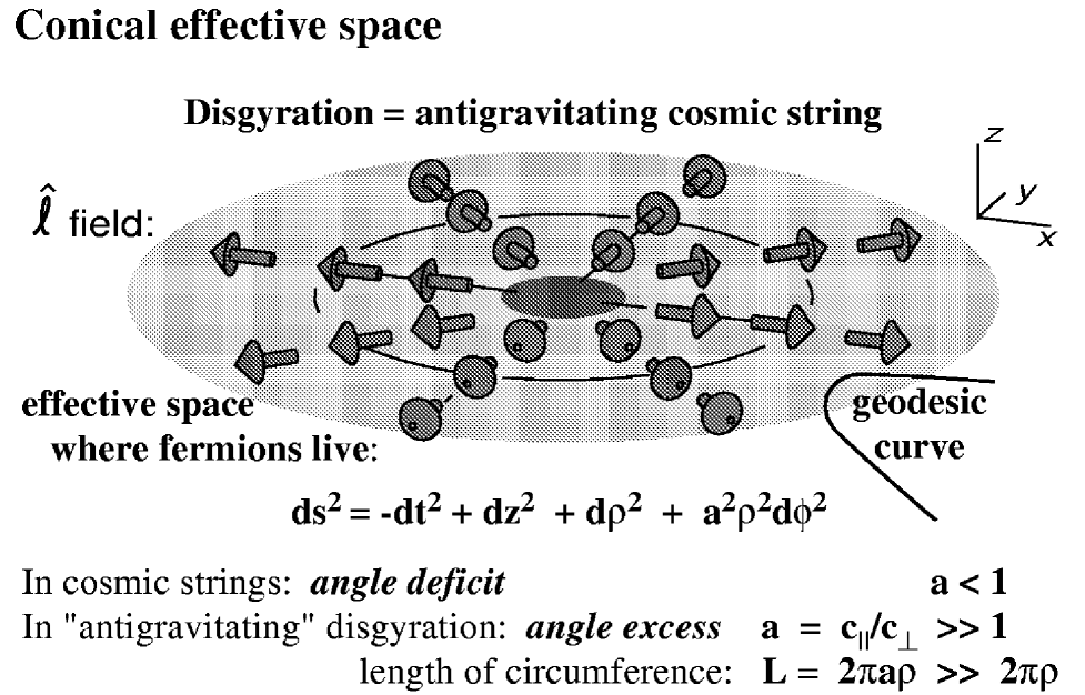
FIG. 19.: The radial disgyration in ³He-A is equivalent to cosmic string with an excess angle. Since all the geodesic curves are repelling from the string, the dysgyration serves as an example of the antigravitating string.

Rescaling the radial and axial coordinates $\rho=c_{\parallel}R$ , $z=c_{\perp}Z$ one obtains

$$ds^{2}=dt^{2}-dZ^{2}-dR^{2}-a^{2}R^{2}d\phi^{2}~{}~{},~{}~{}a^{2}=c_{\parallel}^{2}/c_{\perp}^{2}>1.$$ (306)

In relativistic theories such conical metric, but with $a^{2}<1$, arises outside the local strings. The space outside the string core is flat, but the proper length $2\pi Ra$ of the circumference of radius $R$ around the axis is smaller than $2\pi R$, if $a<1$. This is so called angle deficit. In our case we have $a^{2}>1$, i.e. the ”negative angle deficit”. The conical singularity gives rise to the curvarture which is concentrated at the axis of disgyration ($R=0$) [156, 157]:

$${\cal R}^{R\phi}_{R\phi}=2\pi{a-1\over a}\delta_{2}({\bf R})~{}~{},~{}~{}\delta_{2}({\bf R})=\delta(X)\delta(Y).$$ (307)

Such metric can arise from the Einstein equations for the local cosmic string with the singular energy density concentrated in the string core

$${\cal T}^{0}_{0}={1-a\over 4Ga}\delta_{2}({\bf R})~{}~{}.$$ (308)

where $G$ is the gravitational constant. Since $a=c_{\parallel}/c_{\perp}\gg 1$, this should be rather unusual cosmic string with a large negative mass of Planck scale, i.e. this string is antigravitating – the trajectories of the particles are repelled from the string (Fig. 19).

2 Estimation of Newton constant.

If one finds such singular contribution to the energy density of ³He-A in the presence of radial disgyration one can extract the value of the effective gravitational constant in ³He-A for this particular case.

Let us consider the following Ansatz for the dreibein in the core of the radial disgyration:

$${\bf e}_{2}=c_{\perp}\hat{\bf z}~{}~{},~{}~{}{\bf e}_{1}=f(\rho)c_{\perp}\hat{\bf\phi}~{}~{},~{}~{}f(\rho=0)=0~{}~{},~{}~{}f(\rho=\infty)=1~{}~{},$$ (309)

which corresponds to the effective metric

$$ds^{2}=dt^{2}-dZ^{2}-dR^{2}-{a^{2}\over f^{2}(Rc_{\parallel})}R^{2}d\phi^{2}~{}~{}.$$ (310)

The function $f(\rho)$ can be obtained from the Ginzburg-Landau free energy functional, Eq.(5.4) + Eq.(7.17) in [13], which for the chosen Anzats Eq.(309) has the form

$$F=K{v_{F}p_{F}^{2}\over 96\pi^{2}}\int_{0}^{z_{0}}dz\int_{\rho<\rho_{0}}d^{2}\rho\left[\Lambda(1-f^{2})^{2}+{f^{2}\over\rho^{2}}+\left({df\over d\rho}\right)^{2}\right]-$$ (311)

$$-Kz_{0}{v_{F}p_{F}^{2}\over 48\pi}\int_{0}^{\rho_{0}}d\rho{d(f^{2})\over d\rho}~{}~{}.$$ (312)

Here $\rho_{0}$ and $z_{0}$ are the radius and the height of the cylindrical vessel with the disgyration on the axis; $\Lambda\sim\Delta_{0}^{2}(T)/v_{F}^{2}$; the overall dimensionless factor $K$ in the Ginzburg- Landau region close to the transition temperature $T_{c}$ is

$$K(T)=1-{T^{2}\over T_{c}^{2}}~{}~{},~{}~{}T\rightarrow T_{c}~{}.$$ (313)

The Eq.(311) is some kind of the dilaton field. The Eq.(312) is the pure divergence and thus can be represented as the singular term, which does not depend on the exact structure of the disgyration core, but nevertheless contributes the core energy:

$${\cal F}_{\rm div}=-2\pi K{v_{F}k_{F}^{2}\over 96\pi^{2}}\delta_{2}({\bf\rho})~{}~{},~{}~{}F_{\rm div}=\int d^{3}x{\cal F}_{\rm div}=-K{v_{F}k_{F}^{2}\over 48\pi}~{}~{}.$$ (314)

Now let us extract the “Newton’s constant” $G$ for ³He-A by comparing this core energy with the string mass $M$ obtained by integration of ${\cal T}^{0}_{0}$:

$$M=\int d^{3}X\sqrt{-g}{\cal T}^{0}_{0}={1-a\over 4G}Z_{0}~{}~{}.$$ (315)

Translating this to the ³He-A language, where the “proper” length is $Z_{0}=z_{0}/c_{\perp}$, and taking into account that $a=c_{\parallel}/c_{\perp}\gg 1$ one has

$$M=-{c_{\parallel}\over 4Gc_{\perp}^{2}}z_{0}~{}~{}.$$ (316)

Then from equation, $F_{\rm div}=M$, one obtains the “gravitational constant”

$$G(T)={12\pi\over K(T)\Delta^{2}(T)}~{}.$$ (317)

The same value is obtained from the energy-momentum tensor for the analog of the graviton in ³He-A. $G(T)$ is inversely proportional to the square of the “Planck” energy scale $\Delta_{0}(T)$ and depends on $T$ increasing with $T$, which corresponds to the vacuum screening of the gravity. The temperature dependence of the gravitational constant leads to its time dependence during the evolution of the Universe. The latter has been heavily discussed starting with the Dirac proposal (see Review[158]).

Though we cannot extrapolate the temperature dependence of $K(T)$ in Eq.(313) to the low $T$, we can expect that the overall temperature dependence of the Newton’s constant can be approximated by

$$G(T)\sim G(T=0)\left(1-{T^{2}\over T^{2}_{c}}\right)^{-2}~{},~{}G(T=0)\sim{1\over T_{c}^{2}}\sim{1\over\Delta_{0}^{2}(0)}~{}.$$ (318)

An exact value of $G$ in the low-$T$ regime will be discussed later in Sec.XIV.

Note also that negative mass $M$ in Eq.(316) does not mean that the vacuum in ³He-A is unstable towards formation of the string: the energy of the radial disgyration is dominated by the positive energy term in Eq.(311) which comes from the “Planckian” physics:

$$E_{\rm disg}(\rho_{0})=K{v_{F}k_{F}^{2}\over 48\pi}z_{0}\ln{\rho_{0}\Delta_{0}\over c_{\parallel}}~{}~{}.$$ (319)

C Vortex vs spinning cosmic string.

Another example of the linear topological defects in the vierbein field is the quantized vortex in ³He-A (Fig. 20). In its simplest realization, which occurs, say, in ³He-A films, where the $\hat{\bf l}$ is fixed by the boundary conditions, the vortex structure is given by Eq.(194). It can be laso written in terms of the zweibein vectors ${\bf e}_{1}$ and ${\bf e}_{2}$, which are rotating by $2\pi$ around the origin

$${\hat{\bf l}}={\hat{\bf z}}~{},~{}{\bf e}_{1}=f(\rho)c_{\perp}\hat{\bf\rho}~{},~{}{\bf e}_{2}=f(\rho)c_{\perp}\hat{\bf\phi}~{},~{}f(0)=0~{},~{}f(\infty)=1.$$ (320)

From the definition of the superfluid velocity in Eq.(100) one obtains

$${\bf v}_{\rm s}={\hbar\over 2m\rho}\hat{\bf\phi}~{},~{}\oint d{\bf x}\cdot{\bf v}_{\rm s}\equiv\kappa={\pi\hbar\over m}.$$ (321)

For the general vortex in ³He-A in the parallel-plate geometry with fixed $\hat{\bf l}$, the circulation $\kappa=n_{1}\pi\hbar/m$, where $n_{1}$ can be integer or half-integer ($n_{1}=1/2$ for half-quantum vortex, Alice string in Sec. IX A 6[154]). For vortices in superfluid ⁴He one has $\kappa=n_{1}(2\pi\hbar/m)$ with integer $n_{1}$.

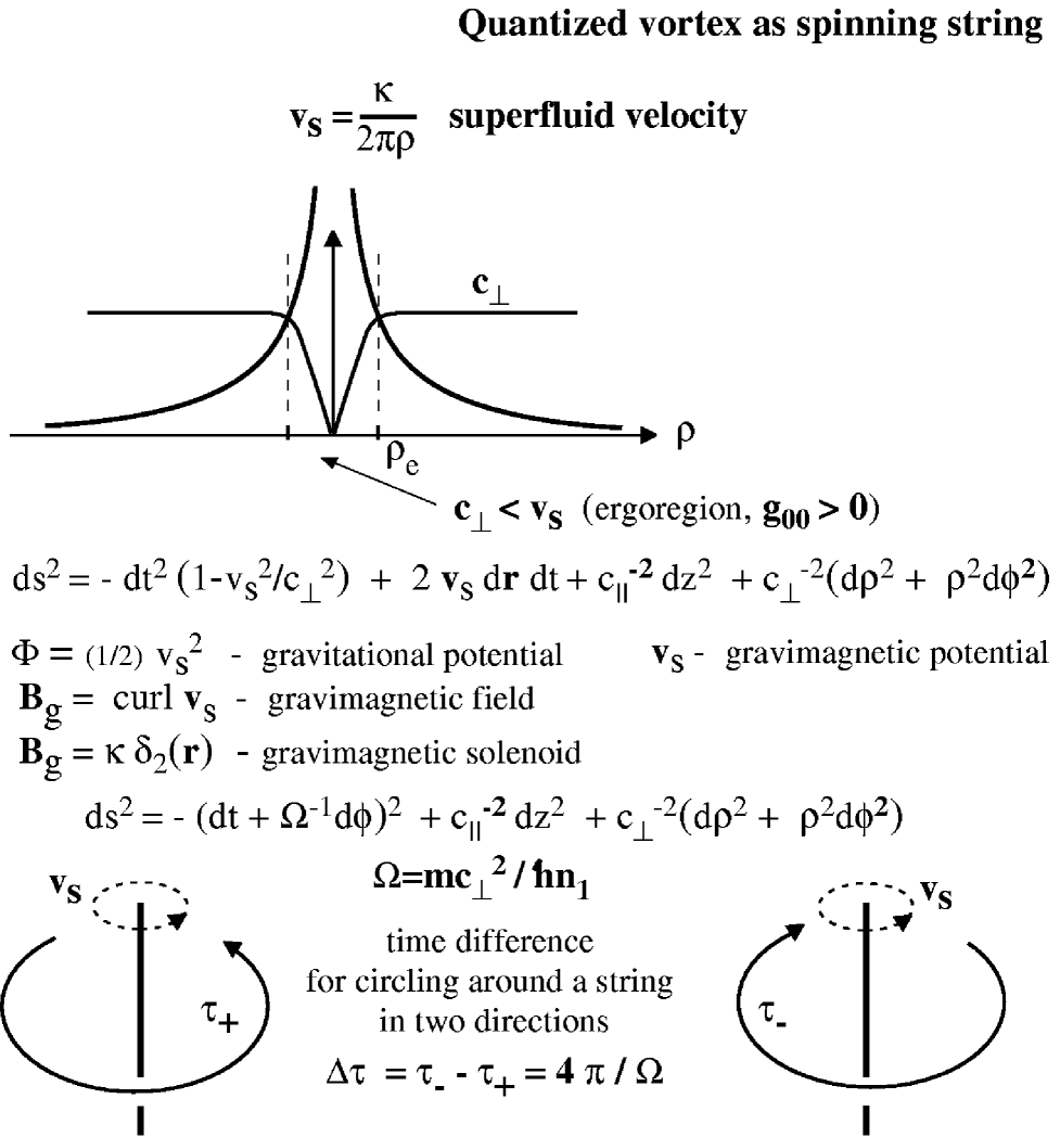
FIG. 20.: The effective metric produced by superflow circulationg around the vortex is similar to the metric of spinning string. bottom: As for the spinning string, there is a constant time difference for the quasiparticle circling with the “speed of light” around the vortex in clockwise and anticlockwise directions. The string serves as a gravimagnetic solenoid and quasiparticles experience the gravitational Aharonov-Bohm effects, which leads to the additional Iordanskii force acting on a vortex.

The superfluid velocity field leads to Doppler shift of the quasiparticle energy which in the low-energy limit modifies the effective metric according to Eq.(106). The azimuthal flow around the core induces the effective space, where quasiparticles propagate along geodesic curves, with the interval

$$ds^{2}=-\left(1-{v_{\rm s}^{2}\over c_{\perp}^{2}}\right)\left(dt+{\kappa d\phi\over 2\pi(c_{\perp}^{2}-v_{\rm s}^{2})}\right)^{2}+{d\rho^{2}\over c_{\perp}^{2}}+{\rho^{2}d\phi^{2}\over c_{\perp}^{2}-v_{\rm s}^{2}}+{dz^{2}\over c_{\parallel}^{2}}~{}.$$ (322)

The same metric is applicable for phonons propagating around the vortex in superfluid ⁴He after the isotropic “speed of light” is introduced, $c_{\perp}=c_{\parallel}=c$.

Far from the vortex, where $v_{\rm s}^{2}/c_{\perp}^{2}$ is small and can be neglected, one has

$$ds^{2}=-\left(dt+{d\phi\over\omega}\right)^{2}+{1\over c_{\perp}^{2}}(d\rho^{2}+\rho^{2}d\phi^{2})+{1\over c_{\parallel}^{2}}dz^{2}~{}~{},~{}~{}\omega={2\pi c_{\perp}^{2}\over\kappa}$$ (323)

The connection between the time and the azimuthal angle $\phi$ in the interval suggests that there is a charactiristic angular velocity $\omega$. For the phonons around the vortex in superfluid ⁴He $\omega=mc^{2}/n_{1}\hbar$, while for the ³He-A fermions $\omega=2mc_{\perp}^{2}/n_{1}\hbar$. The similar metric with rotation was obtained for the so-called spinning cosmic string in $3+1$ space-time, which has the rotational angular momentum $J$ concentrated in the string core, and for the spinning particle in the 2+1 gravity [159, 160, 161, 162]:

$$ds^{2}=-\left(dt+{d\phi\over\omega}\right)^{2}+{1\over c^{2}}(dz^{2}+d\rho^{2}+\rho^{2}d\phi^{2})~{}~{},~{}~{}\omega={1\over 4JG}$$ (324)

where $G$ is the gravitational constant. This gives the following correspondence between the circulation $\kappa$ around the vortex and the angular momentum $J$ of the spinning string

$$\kappa=8\pi JG~{}.$$ (325)

Thus vortices in superfluids simulate the spinning cosmic strings [163].

The effect peculiar for the spinning string, which was modelled in condensed matter, is the gravitational AB topological effect [159]. Outside the string the metric, which enters the interval $ds$, is locally flat. But there is the time difference for the particles propagating around the spinning string in the opposite directions (Fig. 20, bottom). Let us consider the classical propagation of light along the circumference of radius $R$ assuming that there is confinement potential (mirrors). Then the trajectories of phonons (null geodesics) at $\rho=R$ and $z=0$ are described by the equation $ds^{2}=0$, which at large distances from the core, $R\gg c/\omega$, are the cw and ccw rotations with angular velocities

$$\dot{\phi}_{\pm}={1\over\pm{R\over c}-{1\over\omega}}$$ (326)

The difference in the periods $T_{\pm}=2\pi/\dot{\phi}_{\pm}$ for cw and ccw motion of the phonon is [164]

$$2\tau={4\pi\over\omega}~{}~{}.$$ (327)

The apparent “speed of light” measured by the internal observer is also different for “light” propagating in opposite directions $c_{\pm}\approx c(1\pm c/\omega R)$.

This asymmetry between the particles moving on different sides of the vortex is the origin of the Iordanskii force acting on the vortex from the heat bath of quasiparticles (“matter”), which we discuss in the next Section. On the quantum level, the connection between the time variable $t$ and the angle variable $\phi$ in the metric Eq.(324) implies that the scattering cross section of phonons (photons) on the vortex should be the periodic function of the energy with the period equal to $\hbar\omega$. The asymmetric part of this cross section gives rise to the Iordanskii force.

It appears also, that even apart from the effective metric, the condensed matter vortices and global spinning strings have the similar properties. In particular, the spinning string generates the density of the angular momentum in the vacuum outside the string [165]. The angular momentum of the superfluid vacuum outside the vortex is also nonzero and equals ${\bf L}=\int d^{3}x~{}{\bf r}\times n{\bf v}_{\rm s}$. For vortices in superfluid ⁴He this gives the density of the angular momentum $n_{1}\hbar\hat{\bf z}$ per ⁴He atom.

XII Gravitational Aharonov-Bohm effect and Iordanskii force.

A Gravitational Aharonov-Bohm effect.

As we discussed in Secs. VII D and VII E, in superfluids, with their two-fluid hydrodynamics (for superfluid vacuum and quasiparticle, which play the part of matter) there are 3 different topological contributions to the force acting on the quantized vortex [166]. The more familiar Magnus force arises when the vortex moves with respect to the superfluid vacuum. For the relativistic cosmic string such force is absent since the corresponding superfluid density of the quantum physical vacuum is zero. However the analog of this force appears if the cosmic string moves in the uniform background charge density [163, 167]. The other two forces of topological origin also have analogs for the cosmic strings: one of them comes from the analog of the axial anomaly in the core of electroweak string (see Sec.VII C), and another one – the Iordanskii force [169] – comes from the analog of the gravitational Aharonov-Bohm effect [168, 16] experienced by the spinning cosmic string discussed in the previous Section. The connection between the Iordanskii force and conventional Aharonov-Bohm effect was developed in [170, 171, 172].

The Iordanskii force arises when the vortex moves with respect to the heat bath of excitations (“matter”). As we have seen from the Eq.(324) there is a peculiar space-time metric around the spinning string. This metric is locally flat, but its global properties lead due to the time delay for any particle orbiting around the string with the same speed, but in opposite directions, according to Eq.(327). This gives rise to the quantum gravitational Aharonov-Bohm effect [159, 174, 160]. We discuss here how the same effect leads to the asymmetry in the scattering of particles on the spinning string and finally to the Iordanskii lifting force acting on the vortex.

In case of the superfluid ⁴He the equation for phonons with energy $E$ propagating in a curved space-time background created by the vortex follows from the Lagrangian in Eq.(12 for scalar field. If one neglects the change in the particle density around the vortex, one has

$${1\over c^{2}}\left(E-i{\bf v}_{\rm s}\cdot\nabla\right)^{2}\alpha+\nabla^{2}\alpha=0~{}.$$ (328)

In the asymptotic region the quadratic terms ${\bf v}_{\rm s}^{2}/c^{2}$ can be neglected and this equation can be rewritten as [171]

$$E^{2}\alpha-c^{2}\left(-i\nabla+{E\over c}{\bf v}_{\rm s}({\bf r})\right)^{2}\alpha=0~{}~{}.$$ (329)

This equation maps the problem under discussion to the Aharonov-Bohm (AB) problem for the magnetic flux tube [173] with the vector potential ${\bf A}={\bf v}_{\rm s}$, where the electric charge $e$ is substituted by the mass $E/c^{2}$ of the particle [174, 165, 175].

The symmetric part of the scattering cross section of quasiparticle with energy $E$ in the background of the vortex is [171]:

$${d\sigma_{\parallel}\over d\theta}={\hbar c\over 2\pi E}\cot^{2}{\theta\over 2}~{}\sin^{2}{\pi E\over\hbar\omega}~{}.$$ (330)

This equation satsifies the periodicity of the cross section as a function of energy with the period $\Delta E=\omega$ as is required by the spinning string metric in Eq.(324). In superfluids the quasiparticle energy are typically small $E\ll\omega$. For small $E$ the result in Eq.(330) was obtained by Fetter [176]. The generalization of the Fetter result for the quasiparticles with arbitrary spectrum $E({\bf p})$ (rotons in ⁴He and the Bogoliubov-Nambu fermions in superconductors) was recently suggested in Ref.[177]: In our notations it is $d\sigma_{\parallel}/d\theta=(\kappa^{2}p/8\pi v_{G}^{2})\cot^{2}(\theta/2)$, where $v_{G}=dE/dp$ is the group velocity of quasiparticles.

The equation for the particles scattered by the spinning string with zero mass gives was suggested in Refs. [174, 160]:

$${d\sigma_{\parallel}\over d\theta}={\hbar c\over 2\pi E\sin^{2}(\theta/2)}~{}\sin^{2}{\pi E\over\hbar\omega}~{},$$ (331)

It preserves the most important properties of Eq.(330): periodicity in $E$ and singularity at small scattering angle $\theta$.

This singularity at $\theta=0$ is the indication of the existence of the transverse cross-section [172], which leads to the Lorentz force, which acts on the magnetic flux tube in the presence of electric current carried by excitations, and to the Iordanskii force, which acts on the vortex in the presence of the mass current carried by the normal component of the liquid. The asymmetric part in the scattering of the quasiparticles on the velocity field of the vortex has been calculated by Sonin for phonons and rotons in ⁴He [171] and by Cleary [178] for the Bogoliubov-Nambu quasiparticles in conventional superconductors. In the case of “relativistic” phonons the transverse cross section is periodic in the phonon energy $E$ again with the period $\omega$ [171, 172]:

$$\sigma_{\perp}={\hbar\over p}~{}\sin{2\pi E\over\hbar\omega}$$ (332)

At low $E\ll\omega$ this result was generalized for arbitrary excitations with the spectrum $\tilde{E}({\bf p})=E({\bf p})+{\bf p}\cdot{\bf v}_{\rm s}$ moving in the background of the velocity field ${\bf v}_{\rm s}$ around the vortex, using a simple classical theory of scattering [171]. Far from the vortex, where the circulating velocity is small, the trajectory of the quasiparticle is almost the straight line parallel, say, to the axis $y$, with the distance from the vortex line being the impact parameter $x$. It moves along this line with the almost constant momentum $p_{y}\approx p$ and almost constant group velocity $v_{G}=dE/dp$. The change in the transverse momentum during this motion is determined by the Hamiltonian equation $dp_{x}/dt=-\partial\tilde{E}/\partial x=-p_{y}\partial v_{{\rm s}y}/\partial x$, or $dp_{x}/dy=-(p/v_{G})\partial v_{{\rm s}y}/\partial x$. The transverse cross section is obtained by integration of $\Delta p_{x}/p$ over the impact parameter $x$:

$$\sigma_{\perp}=\int_{-\infty}^{+\infty}{dx\over v_{G}}\int_{-\infty}^{+\infty}dy{\partial v_{{\rm s}y}\over\partial x}={\kappa\over v_{G}}~{}.$$ (333)

For $g_{G}=c$ this is the result of Eq.(332) at $E\ll\omega$. Note that the result in Eq.(333) is pure classical: the Planck constant $\hbar$ drops out.

B Iordanskii force on spinning string.

This asymmetric part of scattering, which describes the momentum transfer in the transverse direction, after integration over the distribution of excitations gives rise to the transverse force acting on the vortex if the vortex moves with respect to the normal component. This is the Iordanskii force:

$${\bf F}_{\rm Iordanskii}=\int{d^{3}p\over(2\pi)^{3}}\sigma_{\perp}(p)v_{G}f({\bf p}){\bf p}\times{\hat{\bf z}}=$$ (334)

$$-\kappa{\hat{\bf z}}\times\int{d^{3}p\over(2\pi)^{3}}f({\bf p}){\bf p}=\kappa{\bf P}\times{\hat{\bf z}}$$ (335)

It depends only on the momentum density ${\bf P}$ carried by excitations (matter) and on the circulation $\kappa$ around the vortex. This confirms the topological origin of this force. In the case of the equilibrium distribution of quasiparticles one has ${\bf P}=mn_{\rm n}({\bf v}_{n}-{\bf v}_{\rm s})$. The same Iordanskii force must act on the spinning cosmic string, when it moves with respect to the matter.

Iordanskii force has been experimentally identified in the rotating superfluid ³He-B (Fig. 17). According to the theory for the transport of vortices in ³He-B (Sec.VII E), the Iordanskii force completely determines the mutual friction parameter $d_{\perp}\approx-n_{\rm n}/n_{\rm s}$ at low $T$ (see Sec. IX B 2), where the spectral flow is completely suppressed. This is in accordance with the experimental data, which show that $d_{\perp}$ does approach its negative asymptote at low $T$ [179]. At higher $T$ the spectral flow becomes dominating which leads to the sign reversal of $d_{\perp}$. The observed negative sign of $d_{\perp}$ at low $T$ provides the experimental verification of the analog of the gravitational Aharonov-Bohm effect on spinning cosmic string.

XIII Horizons, ergoregions, degenerate metric, vacuum instability and all that.

A Event horizons in vierbein wall and Hawking radiation.

Let us consider the vierbein wall discussed in Sec. XI A, which is still stationary but there is a superflow across the wall with the superfluid velocity ${\bf v}_{\rm s}=v_{\rm s}\hat{\bf x}$ (Fig. 21). The line element of the effective space-time in Eq.(276) becomes [151]

$$ds^{2}=-dt^{2}+{1\over c^{2}(x)}(dx-v_{\rm s}dt)^{2}+{1\over c_{\perp}^{2}}dy^{2}+{1\over c_{\parallel}^{2}}dz^{2}=$$ (336)

$$-\left(1-{v_{\rm s}^{2}\over c^{2}(x)}\right)\left(dt+{v_{\rm s}dx\over c^{2}(x)-v_{\rm s}^{2}}\right)^{2}+{dx^{2}\over c^{2}(x)-v_{\rm s}^{2}}~{},~{}c(x)=c_{\perp}\tanh{x\over d}~{}.$$ (337)

In Eq.(337) we omitted the irrelevant metric of the space along the wall.

FIG. 21.: When there is a superflow across the soliton, the vierbein wall splits into a pair of horizons: black hole and white hole. Between the horizons the superfluid velocity exceeds the “speed of light” and $g_{00}$ changes sign. Since their speed $c^{x}$ is smaller that the velocity of the superfluid vacuum, the “relativistic” quasiparticles within the horizon can move only along the streamlines. Horizon at $x=-x_{h}$ is the black-hole horizon, since no information can be extracted from the region behind this horizon, if the low-energy quasiparticles are used for communication.

The naive transformation

$$\tilde{t}=t+\int^{x}{v_{\rm s}dx\over c^{2}(x)-v_{\rm s}^{2}}$$ (338)

in Eq.(337) gives

$$ds^{2}=-\left(1-{v_{\rm s}^{2}\over c^{2}(x)}\right)d\tilde{t}^{2}+{dx^{2}\over c^{2}(x)-v_{\rm s}^{2}}~{}.$$ (339)

This line element corresponds to the radial part of the Schwarzschild metric for the black hole. The metric in Eq.(339) shows that there are two horizons in the soliton: at planes $x_{h}$ where $c(x_{h})=v_{\rm s}$ and at $x_{-}=-x_{h}$ where $c(-x_{h})=-v_{\rm s}$. This “Schwarzschild” metric has coordinate singularity at horizons and thus is not determined globally, this is because the transformation in Eq.(338) is ill defined at the horizons. The “Schwarzschild” metric can describe the effective space time either outside the horizons or between them, at $-x_{h}<x<x_{h}$

The original metric in Eq.(336) is well determined everywhere except for the physical singularity at $x=0$, where the vierbein is degenerate). This is because in the effective gravity theory in ³He-A (and also in superfluid ⁴He) the primary quantity is not the metric, but the energy spectrum of quasiparticle, which in the low energy corner becomes “relativistic” and acquires the Lorentzian form, thus giving rise to the contravariant metric $g^{\mu\nu}$. Then from this contravariant metric, if it is nondegenerate, the covariant metric $g_{\mu\nu}$ is obtained which describes the effective space-time. Thus only those space-times are physical in these effective theories, which came from the physically reasonable quasiparticle spectrum. Since the spectrum of quasiparticles must be determined everywhere, if the vacuum state is locally stable, the contravariant effective metric $g^{\mu\nu}$ is well determined in the whole underlying Galilean space time of the condensed matter. As a result the covariant effective metric $g_{\mu\nu}$, which determines the line element of the effective space-time, must be also determined everywhere except for the places where the the contravariant metric $g^{\mu\nu}$ is degenerate. The spectrum of the ³He-A fermionic quasiparticles, which gives rise to the effective metric in Eq.(336) is

$$\tilde{E}_{a}({\bf p})=E_{a}({\bf p})+p_{x}v_{\rm s}~{},~{}E_{a}({\bf p})=\pm\sqrt{c_{\parallel}^{2}(p_{z}-e_{a}p_{F})^{2}+c_{\perp}^{2}p_{y}^{2}+c^{2}(x)p_{x}^{2}}$$ (340)

which as we know can be written in the Lorentzian form $g^{\mu\nu}(p_{\mu}-e_{a}A_{\mu})(p_{\nu}-e_{a}A_{\nu})=0$.

Inspection of the energy spectrum of quasiparticles in Eq.(340) or of the metric in Eq.(336) shows that the two horizons, at $x=x_{h}$ and at $x=-x_{h}$, are essentially different. The horizon at $x=-x_{h}$ represents the black hole horizon, while that at $x=x_{h}$ is the white hole horizon. This is because in the region between the horizons, at $-x_{h}<x<x_{h}$, the group velocity of the quasiparticle in the soliton frame $v_{Gx}=d\tilde{E}({\bf p})/dp_{x}=dE({\bf p})/dp_{x}+v_{\rm s}$ is positive for both directions of the quasiparticle momentum $p_{x}$ (see Fig. 21, where the superfluid velocity $v_{\rm s}$ is chosen positive). All the (low-energy) quasiparticles inside the horizon will finally cross the plane $x=x_{h}$, which means that this plane is the white hole horizon. But the quasiparticles cannot cross the plane $x=-x_{h}$ from inside, which indicates the black hole horizon: The “inner” observer living at $x<-x_{h}$ cannot obtain the information from the region $x>-x_{h}$, if he uses the “relativistic” quasiparticles for communication.

Appearance of pairs of the white-hole/black-hole horizons is typical for the condensed matter.

In the presence of horizons the notion of the vacuum state becomes subtle. There are two important reference frames in which the vacuum state can be defined: they give the same definition of the vacuum if there are no horizons, but in the presence of the horizons the two vacua do not coincide.

(i) The superfluid-comoving vacuum. This is the vacuum as seen by the local “inner” observer, who is comoving with the superfluid component, i.e. moving with the velocity ${\bf v}_{\rm s}$. This vacuum is regulated by the energy $E({\bf p})$ in Eq.(340): the states with the negative root in Eq.(340) are occupied. This vacuum state can be also determined as the limit of the local thermal state in Eq.(47) if $T\rightarrow 0$ at zero counterflow velocity, $w=0$, or at any fixed “subluminal” counterflow velocity, $w<c$. Such vacuum, however, cannot be defined globally, because in the reference moving with the superfluid velocity, the metric is time dependent.

(ii) The texture-comoving vacuum. This is the vacuum as determined in the frame of the wall, where the metric does not depend on time (in general relativity this means that the spacetime determined by such metric has a global timelike Killing vector). Since there is no time dependence, the quasiparticle energy is well defined globally as $\tilde{E}({\bf p})$. The vacuum is determined as the state in which the energy levels with $\tilde{E}({\bf p})<0$ are occupied.

In the presence of the horizons the superfluid-comoving vacuum and the texture-comoving vacuum do not coincide in the region between the horizons. Some energy states with the positive root in Eq.(340), which were empty before, acquire in the texture-comoving frame the negative energy in the presence of the horizons and must be occupied. The process of the filling of the negative energy levels is governed by the spatial inhomogeneity, since for the homogeneous system there is no preferred frame and the “inner” observer does not know at $T=0$ whether the liquid is moving or not. The inhomogeneity is provided by the spatial dependence of the metric within the soliton. Thus the process of the dissipation of the superfluid-comoving vacuum is determined by the derivatives of the texture, in a given case by the gradient of the “speed of light” $c(x)$, or equivalently by the gradient of the metric, which plays the part of the gravitational field.

An example of the dissipation, caused by the gradients of the metric, is the Hawking radiation of quasiparticles [180]. This radiation is characterized by the Hawking temperature, which depends on the gradient of the “speed of light” or, in terms of the gravity theory, by the “surface gravity” $\kappa_{S}$ at the horizon:

$$T_{\rm H}={\hbar\over 2\pi}\kappa_{S}~{},~{}\kappa_{S}=\left({dc\over dx}\right)_{h}~{}~{}.$$ (341)

In the case of Eq.(337) for the profile of the “speed of light” the Hawking temperature depends on the velocity $v_{\rm s}$:

$$T_{\rm H}(v_{\rm s})=T_{\rm H}(v_{\rm s}=0)\left(1-{v_{\rm s}^{2}\over c_{\perp}^{2}}\right)~{}~{}~{},~{}~{}~{}T_{\rm H}(v_{\rm s}=0)={\hbar c_{\perp}\over 2\pi d}~{}.$$ (342)

Typically for this type of domain wall the Hawking temperature $T_{\rm H}(v_{\rm s}=0)$ is below $1~{}\mu K$; the Hawking flux of radiation could in prinicple be detected by quasiparticle detectors.

The Hawking radiation leads to the energy dissipation and thus to the quantum friction, which decreases the velocity $|v_{\rm s}|$ of the domain wall with respect to the superfluid vacuum. Due to the deceleration of the wall motion, the Hawking temperature increases with time. The distance between horizons, $2x_{h}$, decreases until the complete stop of the domain wall when the two horizons merge. The Hawking temperature approaches its asymptotic value $T_{\rm H}(v_{\rm s}=0)$ in Eq.(342); but when the horizons merge, the Hawking radiation disappears: there is no more ergoregion (region with negative energy states), so that the stationary domain wall is nondissipative, as it should be.

Actually all this is valid when the quasiparticle spectrum near the domain wall can be considered as continuous. The quasiparticle spectrum in Eq.(340) takes place only if the horizons a far apart, i.e. the distance between them is much larger than the superfluid coherence length, $x_{H}\gg v_{F}/\Delta_{0}$. This is satisfied when the relative velocity between the domain wall and the superfluid vacuum is close to $c_{\perp}$, so that $x_{h}\sim(d/2)\ln[1/(1-v_{\rm s}^{2}/c_{\perp}^{2})]\gg d$. Thus the dissipation stops when the distance between the horizon becomes comparable to the “Planck length” $\xi=c_{\parallel}/\Delta_{0}$. Also the Hawking radiation is only one of the possible mechanisms of the dissipation: the real scenario of the relaxation of the horizons depends on the details of the back reaction of the superfluid vacuum to the filling of the negative energy states.

B Landau critical velocity and ergoregion

The horizons, discussed in the previous subsection, appeared as surfaces where the superfluid velocity approached the “speed of light” $c_{\perp}$. In general, i.e. for the “nonrelativistic” spectrum of quasiparticles, the quantum friction in superfluids starts when the superfluid velocity exceeds the Landau critical velocity

$$v_{\rm Landau}={\rm min}{E({\bf p})\over p}~{}.$$ (343)

Above this velocity the energy $\tilde{E}({\bf p})=E({\bf p})+{\bf p}\cdot{\bf v}_{\rm s}$ of some excitations, as measured in the laboratory frame (or in the frame of the moving soliton), becomes negative. This allows for excitations to be nucleated from the vacuum. For a superfluid velocity field which is time-independent in the laboratory (or soliton) frame, the region where $v_{\rm s}({\bf r})>v_{\rm Landau}$ and quasiparticles can have negative energy, is called the ergoregion. The surface $v_{\rm s}({\bf r})=v_{\rm Landau}$ which bounds the ergoregion, is called the ergosurface.

In a given geometry discussed in previous subsection the “speed of light” coincides with the Landau critical velocity, if only the “relativistic” quasiparticles are considered. Also the horizons coincide with the ergosurfaces, as it happens for the nonrotating black hole. For the general superflow (or for the different type of the soliton [181]) horizon and ergosurface are separated from each other, as in the case of the rotating black hole.

In general, however, the behavior of the system depends crucially on the dispersion of the spectrum at higher energy. There are two possible cases.

(1) The spectrum bends upwards at high energy, i.e. $E({\bf p})=cp+\gamma p^{3}$ with $\gamma>0$. Such dispersion can be realized for the fermionic quasiparticles in ³He-A, for example from Eq.(297) it follows that $\gamma^{-1}=8(m^{*})^{2}c_{\perp}$. Quasiparticles are “relativistic” in the low energy corner but become “superluminal” at higher energy [151, 181]. In this case the Landau critical velocity coincides with the “speed of light”, $v_{\rm Landau}=c$, so that the ergosurface is determined by $v_{\rm s}({\bf r})=c$. In the Lorentz invariant limit of the energy much below the “Planck” scale, i.e. at $p^{2}\ll\gamma/c$ (or $p\ll m^{*}c_{\perp}$) this corresponds to the ergosurface at $g_{00}({\bf r})=0$, which is just the definition of the ergosurface in gravity. In case of radial flow of the superfluid vacuum towards the origin (Fig. 22), the ergosurface also represents the horizon in the Lorentz invariant limit, and the region inside the horizon simulates a black hole for low energy quasiparticles. Strictly speaking this is not a true horizon for quasiparticles: Due to the nonlinear dispersion, their group velocity $v_{G}=dE/dp=c+3\gamma p^{2}>c$, and thus the high energy quasiparticles are allowed to leave the black hole region. It is, hence, a horizon only for quasiparticles living exclusively in the very low energy corner: they are not aware of the possibility of “superluminal” motion. Nevertheless, the mere possibility to exchange the information across the horizon allows us to construct the thermal state on both sides of the horizon and to investigate its thermodynamics, including the entropy related to the horizon (see Sec. XIII G and Ref. [182]).

(2) In superfluid ⁴He the negative dispersion is realized, $\gamma<0$, with the group velocity $v_{G}=dE/dp<c$ (if one neglects a small upturn of the spectrum at low $p$). In such superfluids the “relativistic” ergosurface $v_{\rm s}({\bf r})=c$ does not coincide with the true ergosurface, which is determined by $v_{\rm s}({\bf r})=v_{\rm Landau}<c$. In superfluid ⁴He, the Landau velocity is related to the roton part of the spectrum, and is about four times less than $c$. In case of radial flow inward, the ergosphere occurs at $v_{\rm s}(r)=v_{\rm Landau}<c$, while the inner surface $v_{\rm s}(r)=c$ still marks the horizon (Fig. 22). This is in contrast to relativistically invariant systems, for which the ergosurface and the horizon coincide for purely radial gravitational field of the chargless nonrotating black hole. The surface $v_{\rm s}(r)=c$ stays a horizon even for excitations with very high momenta up to some critical value, at which the group velocity of quasiparticle again approaches $c$.

C Painlevé-Gullstrand metric in effective gravity in superfluids. Vacuum resistance to formation of horizon.

Let us consider the spherically symmetric radial flow of the superfluid vacuum, which is time-independent in the laboratory frame (Fig. 22). For simplicity let us assume the isotropic “speed of light” as in superfluid ⁴He. Then dynamics of the quasiparticles, propagating in this velocity field, is given by the line element provided by the effective metric in Eq.(37):

$$ds^{2}=-\left(1-{v_{\rm s}^{2}(r)\over c^{2}}\right)dt^{2}+2{v_{\rm s}(r)\over c^{2}}drdt+{1\over c^{2}}(dr^{2}+r^{2}d\Omega^{2})\,.$$ (344)

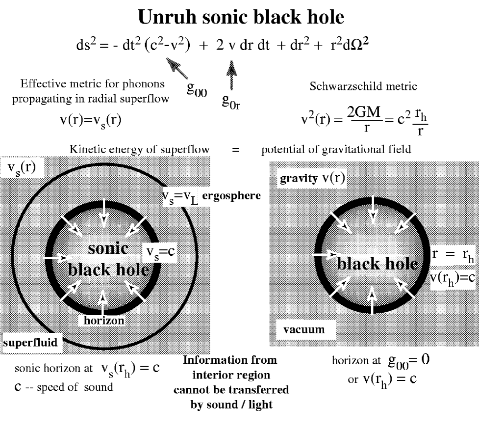
FIG. 22.: Unruh sonic black hole in superfluid ⁴He. The horizon and ergosphere coincide only for the “relativistic” phonons. For the real quasiparticle spectrum the ergosphere occurs when the velocity of flow reaches the Landau velocity for rotons.

This equation corresponds to the Painlevé-Gullstrand line elements. It describes a black hole horizon if the superflow is inward (see refs.[14, 15]; on the pedagogical review of Panlevé-Gullstrand metric see [183]; on the quantum vacuum effects in gravity and in its condensed matter analogs see [184]). If $v_{\rm s}(r)=-c(r_{\rm h}/r)^{1/2}$ the flow simulates the black hole in general relativity. For the outward superflow with, say, $v_{\rm s}(r)=+c(r_{\rm h}/r)^{1/2}$ the white hole is reproduced. For the general radial dependence of the superfluid velocity, the Schwarzschild radius $r_{\rm h}$ is determined as $v_{\rm s}(r_{\rm h})=\pm c$; the “surface gravity” at the Schwarzschild radius is $\kappa_{S}=(1/2c)dv^{2}_{\rm h}/dr|_{r_{S}}$; and the Hawking temperature $T_{\rm H}=\hbar\kappa_{S}/2\pi$.

It is not easy to create the flow in the Bose liquid, which exhbits the horizon for phonons. This is because of the hydrodynamic instability which takes place behind the horizon (see [185, 184]). From Eqs.(1) and (4) of superfluid hydrodynamics at $T=0$ (which correspond to conventional hydrodynamics of ideal curl-free liquid) it follows that for stationary motion of the liquid one has the relation between $n$ and $v_{\rm s}$ along the streamline [186]:

$${\partial(nv_{\rm s})\over\partial v_{\rm s}}=n\left(1-{v_{\rm s}^{2}\over c^{2}}\right)\,.$$ (345)

The current $J=nv_{\rm s}$ has a maximal value just at the horizon and thus it must decrease behind the horizon, where $1-(v_{\rm s}^{2}/c^{2})$ is negative. This is, however, impossible in the radial flow since, according to the continuity equation (1), one has $nv_{\rm s}=Const/r^{2}$ and thus the current must monotonically increase across the horizon. This marks the hydrodynamic instability behind the horizon and shows that it is impossible to construct the time-independent flow with the horizon without the fine-tuning of an external nonhydrodynamic (“nongravitational”) force acting on the liquid [185, 184]. Thus the liquid (vacuum) itself resists to the formation of the horizon.

Would the quantum vacuum always resist to formation of the horizon? Fortunately, not. In the considered case of superfluid ⁴He, the same “speed of light” $c$, which describes the quasipartilces (acoustic waves – phonons) and thus determines the value of the superfluid velocity at horizon, also enters the hydrodynamic equations that establish the flow pattern of the “black hole”. For spin waves the “speed of light” can be less than the hydrodynamic speed of sound, that is why the horizon can be reached before the hydrodynamic instability. In Fermi superfluid ³He-A these two speeds can be well separated. The “speed of light” $c_{\perp}$ for quasiparticles, which determines the velocity of liquid flow at the horizon, is about $c_{\perp}\sim 3$cm/sec, which is much less than the speed of sound $s\sim 200$m/sec, which determines the hydrodynamic instabilities of the liquid. That is why there are no severe hydrodynamic constraints on the flow pattern, the hydrodynamic instability is never reached and the surface gravity at such horizons is always finite.

In superfluids another instability can develop preventing the formation of the horizon. Typically, the “speed of light” $c$ for “relativistic” quasiparticles coincides with the critical velocity, at which the superfluid state of the liquid becomes unstable towards the normal state of the liquid [187]. In this case, when the superfluid velocity with respect to the normal component or to the container walls exceeds $c$, the slope $\partial J/\partial v_{\rm s}$ becomes negative and the superflow becomes locally unstable. The interaction between superfluid vacuum and the walls leads to collapse of the superflow, so that the stationary superflow with $w>c$ is impossible. This instability, however, can be smoothened if the container walls are properly isolated. In Ref.[188] it was suggested to isolate the moving superfluid ³He-A from the walls by the layer of superfluid ⁴He. Then the direct interaction and thus the momentum exchange between the flowing condensate and the container walls is suppressed. The momentum exchange occurs due to the gradients of the velocity field, and can be made slow if the gradients are small, so that the state with the horizon can live long. Since the velocity gradient corresponds to the effective gravitation field, the relaxation of the superflow in the presence of the horizon at the initial stage of the flow instability becomes similar to the Hawking process of the relaxation of the black hole.

In principle, in Fermi superfluids, if the parameters of the system are favourable, the “speed of light” can be made slightly less then the critical velocity at which the superfluid collapses. In this case the superflow can remain stable in a supercritical regime, which means that the state with the horizon can be stabilized: the fermionic quasiparticles formed in the Hawking process finally occupy all the negative energy states and relaxation stops. Let us first consider this final state of stable horizon.

D Stable event horizon and its momentum-space topology.

The horizon can be stabilized due to the nonlinear dispersion of the energy spectrum. This can be illustrated on the simplest case of the motion through the narrow place in the tube (Fig. 23). Let us consider what happens with the system in the system, when we continuously increase the velocity of the superflow from slightly below to slightly above the “speed of light” $c_{\perp}$. Further we consider for simplicity the isotropic superfluid with the nonlinear spectrum $E^{2}(p)=c^{2}p^{2}(1+p^{2}/p_{\rm P}^{2})$. Here we assumed the case of the superluminal dispersion, i.e. $\gamma>0$, and introduced the Planck momentum, which enters the nonlinear dispersion, $p_{\rm P}=\sqrt{c_{\perp}/2\gamma}$. In ³He-A it is of order $m^{*}c_{\perp}$. We shall see that in some cases only this first nonlinear correction does the whole job, so that the characteristic momenta are concentrated well below the Planck scale, $p\ll p_{\rm P}$, where the higher order corrections are negligibly small.

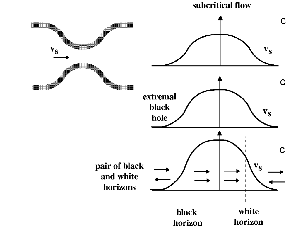
FIG. 23.: The change of the effective space-time when the superfluid velocity through the orifice continuously increases. When $v_{\rm s}$ exceeds the “speed of light” the black-hole/white-hole pair appears. Arrows show possible directions of the quasiparticles in the low-energy “relativistic” limit. Between the horizons these quasiparticles can move only to the right. The intermediate state when the velocity profile first touches the “speed of light”, has the effective metric which is equivalent to that in vicinity of the horizon of extremal black hole.

When $v_{\rm s}$ exceeds the “speed of light” $c$ the pair of horizons, black and white, are formed similar to the case discussed in Sec. XIII. The only difference is that now the superfluid velocity ${\bf v}_{\rm s}$ is space dependent, while the “speed of light” $c$ is constant. The horizons can be considered as planes with coordinate $x$ along the normal to the plane. The interval in the laboratory reference frame, where the metric is time independent, has the form

$$ds^{2}=-\left(1-{v_{\rm s}^{2}(x)\over c^{2}}\right)dt^{2}+2{v_{\rm s}(x)\over c^{2}}dxdt+{1\over c^{2}}(dx^{2}+dy^{2}+dz^{2})\,.$$ (346)

Since the superfluid velocity has a maximum at $x=0$, then in the region of the crossover from subcritical flow to the horizons it can be approximated as

$${v_{\rm s}(x)\over c}=1+{\alpha\over 2}-{x^{2}\over 2x_{0}^{2}}~{},~{}|\alpha|\ll 1~{},$$ (347)

where $x_{0}$ is of order of the dimension of the container. The parameter $\alpha$ regulates the crossover: it changes from small negative value when there are no horizons, to the small positive value, when the two horizons appear.

Within the relativistic limit the system with horizons, i.e. at $\alpha>0$, does not possess the states of global thermodynamic equilibrium (except possibly at the Hawking temperature, which is determined by the quantum effect and is very low). Since in such equilibrium the normal component velocity must be zero in the laboratory frame, the counterflow velocity $w$ exceeds the speed of light in the region between the horizons and thus the thermodynamic potential in Eq.(47) is not determined. However, the nonrelativistic corrections can restore the global thermodynamic equilibrium. The laboratory frame energy spectrum of quasiparticles with the nonlinear dispersion can be written for small $\alpha$ in the following form

$$\tilde{E}=p_{x}v_{\rm s}(x)+E(p)\approx{1\over 2}c|p_{x}|\left({x^{2}\over x_{0}^{2}}-\alpha+{p_{y}^{2}+p_{z}^{2}\over p_{x}^{2}}+{p_{x}^{2}\over p_{\rm P}^{2}}\right)~{},~{}p_{x}<0~{},~{}p_{y}^{2}+p_{z}^{2}\ll p_{x}^{2}~{},~{}|p_{x}|\ll p_{\rm P}~{},$$ (348)

where we took into account that in the relevant low-energy region the quasiparticle momentum is almost antiparallel to the superflow and thus $|p_{x}|\gg p_{\perp}$.

Inspection of the Eq.(348) shows the dramatic change in the topology of the energy spectrum when $\alpha$ crosses zero. At $\alpha<0$, where the superfluid velocity is everywhere subcritical, the energy of quasiparticle is zero only at ${\bf p}=0$ (in real $3$He-A at ${\bf p}=\pm p_{F}\hat{\bf l}$). This is the topologically stable Fermi point discussed in Secs. IV C and V. At $\alpha>0$ the pair of horizons appears at $x=\pm x_{h}$, where $x_{h}=x_{0}\sqrt{\alpha}\ll x_{0}$. As a result the topological invariant for the Fermi point at ${\bf p}=0$ changes from nonzero value ($N_{3}=1$ or $N_{3}=-1$) to $N_{3}=0$. Instead another topologically stable manifold of zeroes arises: this is the Fermi surface, which appears in the region between the horizons, i.e. at $x^{2}<x_{h}^{2}$. The Fermi surface, the surface in momentum space where the quasiparticle energy in Eq.(348) is zero, is determined by equation

$${p_{y}^{2}+p_{z}^{2}\over p_{x}^{2}}+{p_{x}^{2}\over p_{\rm P}^{2}}={x_{h}^{2}-x^{2}\over x_{0}^{2}}~{}~{},~{}~{}-x_{h}<x<x_{h}~{}.$$ (349)

Thus the appearance of the horizons corresponds to the quantum phase transition at which the topology of the quasiparticle spectrum drastically changes.

In the extended space, which includes the momentum ${\bf p}$ and the coordinate $x$, the manifold of zeroes of the quasiparticle energy is the 3D Fermi hypersurface in the 4D space $({\bf p},x)$.

At $\alpha>0$ the quasiparticles start, say by Hawking radiation, to fill the negative energy states within the Fermi surface until all of them become occupied. The state with the Fermi surface is thus the final zero-temperature state of the Hawking radiation. The states of the global thermodynamic equilibrium with nonzero $T$ are also determined by the Fermi surface properties which, according to the conventional rules for the degenerate Fermi system, are determined by the density of states at zero energy. If $\alpha$ is small, the momenta and energies of the occupied states are still small compared to the Planck scale:

$$|p_{x}|\leq p_{\rm P}\alpha^{1/2}\ll p_{\rm P}~{},~{}|p_{y}|\leq p_{\rm P}\alpha\ll p_{\rm P}~{},~{}E\sim cp_{x}\ll E_{\rm P}~{}.$$ (350)

The density of states is thus $\sim p_{x}p_{y}p_{z}/E\sim(p_{\rm P}^{2}/c)\alpha^{2}$.

This is one of the examples when the effect of the Planck physics does not require the knowledge of the details of transPlanckian physics, since only the first nonlinear correction to the energy spectrum determines the phenomenon.

If $\alpha$ is small, the total number of the occupied states, $\sim Ax_{0}p_{\rm P}^{3}\alpha^{2}$, where $A$ is the area of the horizon, is also small. That is why one can expect that at $\alpha\ll 1$ the reconstruction of the vacuum occurs without essential modification of the velocity profile, i.e. without the considerable back reaction of the “gravitational field”. However, this is not so simple. The detailed inspection of the backreaction of the order parameter field to the filling of the negative energy levels shows that the back reaction can be significant: the supercritical state with the Fermi surface is typically unstable towards the collapse of the superfluidity [187]. In such case, there are no true equilibrium states in the presence of the horizon. So that the final result will be the merging and mutual annihilation of the two horizons. This occurs either by the collapse of superfluidity, or, if the collapse is smooothened, by thermal relaxations of the local equilibrium states, which we discuss in Sec.XIII G and at very low temperature by the Hawking radiation.

E Hawking radiation.

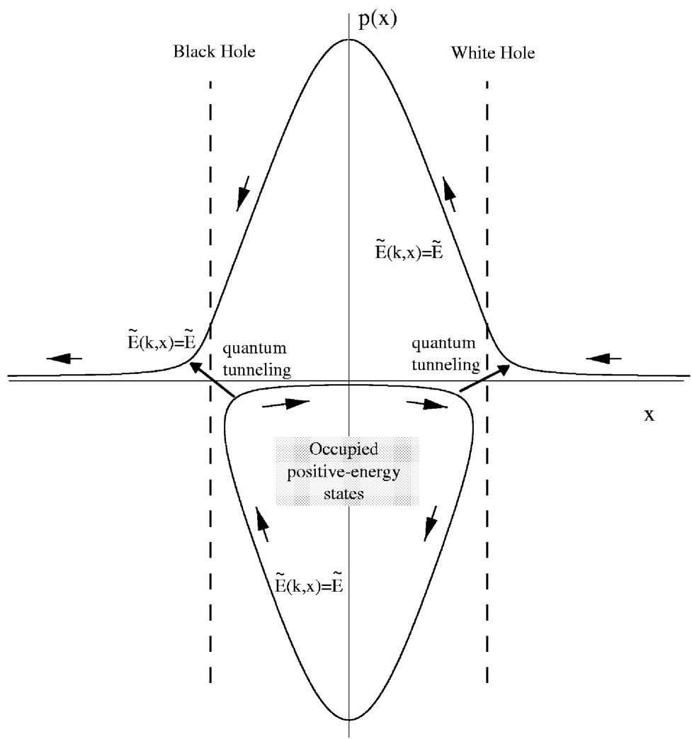
FIG. 24.: Trajectories of quasiparticles in the presence of the black-hole/white-hole pair in $1+1$ case. The nonlinear dispersion of the energy spectrum at high momentum $p$ is taken into account. Only those positive-energy trajectories are considered, which are responsible for the Hawking-like radiation. They are represented by curves of constant energy in the laboratory (Killing) frame: $\tilde{E}(p,x)=\tilde{E}>0$. The trajectory between the horizons has negative energy, $E<0$, in the frame comoving with the superfluid vacuum. That is why the corresponding quantum states are initially occupied. But in the laboratory frame these quasiparticles have positive energy, $\tilde{E}>0$, and thus can tunnel to the mode with the same energy $\tilde{E}>0$, which is out-going from the black hole. The radiation from the black hole also occurs by tunneling to the mode in-going to the white hole, which due to “superluminal” dispersion crosses both horizons.

Fig. 24 shows the relevant classical trajectories of quasiparticles in the presence of the horizons in simplest $1+1$ case. We consider the positive energy states, as veiwed in the laboratory frame, where the velocity field is time-independent. They are given by the equation $\tilde{E}(p,x)=\tilde{E}>0$ with $\tilde{E}(p,x)$ given by Eq.(348). Between the horizons the positive energy states in the laboratory frame have the negative energy as viewed by the inner observer moving with the superfluid velocity ${\bf v}_{\rm s}$: in the “relativistic” domain this energy is $E(p)=-cp<0$. The corresponding quantum states belong to the quantum vacuum as viewed by the comoving observer, that is why these states between the horizons are initially occupied. This comoving vacuum is seen in the absolute laboratory frame as highly excited state withe nonequilibrium distribution of quasiparticles. The equilibrization occurs via tunneling of the quasiparticles from the occupied excited states to the modes with the same positive energy $\tilde{E}(p,x)=\tilde{E}>0$, which is out-going from the black-hole horizon. The tunneling exponent is determined by the usual quasiclassical action $2{\rm Im}\int p(x)dx$. At low energy, when the nonrelativistic corrections are neglected, the momentum as a function of $x$ on the classical trajectory has a pole at the horizon $p(x)\approx\tilde{E}/v^{\prime}_{\rm s}(x-x_{h})$. Here $v^{\prime}_{\rm s}$ is the derivative of the superfluid velocity at the horizon, which is equivalent to the surface gravity. Using the standard prescription for the treating of poles, one obtains for the tunneling action $2{\rm Im}\int p(x)dx=2\pi\tilde{E}/v^{\prime}_{\rm s}$, which is similar to the thermal radiation with the Hawking temperature:

$$T_{\rm H}={\hbar\over 2\pi}\kappa_{S}~{},~{}\kappa_{S}=\left({dv_{\rm s}\over dx}\right)_{h}~{}~{}.$$ (351)

This can be compared with the Eq.(341) for the Hawking temperature in the case of moving soliton in terms of the “surface gravity” $\kappa_{S}$ at the horizon. The only difference is that in the case of soliton the “surface gravity” is simulated by the gradient of the “speed of light” instead of the gradient of the superfluid velocity in Eq.351).

There is another channel of dissipation. According to Fig. 24 the radiation from the region between the horizons also occurs by tunneling to the mode in-going to the white hole. This mode, due to the “superluminal” dispersion, crosses both horizons and is transformed to the mode out-going from the black-hole horizon. The tunneling exponent is given by Eq.(351) where it is now the velocity gradient at the white-hole horizon, which determines the Hawking temperature of this tunneling.

F Extremal black hole.

Let us consider the transition point, $\alpha=0$. After rescaling of the Eq.(346) at $\alpha=0$ one obtains the following interval

$$ds^{2}=-x^{2}dt^{2}+2dxdt+dx^{2}+dy^{2}+dz^{2}=-x^{2}\left(dt-{dx\over x^{2}}\right)^{2}+{dx^{2}\over x^{2}}+dy^{2}+dz^{2}\,.$$ (352)

The plane $x=0$, where the black and white horizons merge, marks the bridge between the two spaces. The metric in Eq.(352) coincides with the metric in the vicinity of the horizon of an extremal black hole, whose mass equal to the electric charge:

$$ds^{2}=-\left(1-{r_{h}\over r}\right)^{2}dt^{2}+\left(1-{r_{h}\over r}\right)^{-2}dr^{2}+r^{2}d\Omega\,.$$ (353)

There is a strong divergency of the effective temperature at the horizon, $T_{\rm eff}\propto T/x$, according to the Tolman’s law in Eq.(52), where $T$ is the constant Tolman’temperature which is a real temperature in superfluids. Because of that all the thermodynamic quantities have singularity at the horizon where the Planck scale of energy must intervene to cut-off the divergency. However, the first nonlinear correction to the “relativistic” energy spectrum provides the necessary cut-off already at low energy, which is much less than the Planck energy scale.

The energy spectrum in the vicinity of the horizon of our extremal black hole is according to Eq.(348)

$$\tilde{E}={1\over 2}cp_{x}\left({x^{2}\over x_{0}^{2}}+{p_{y}^{2}+p_{z}^{2}\over p_{x}^{2}}+{p_{x}^{2}\over p_{\rm P}^{2}}\right)~{},~{}p_{x}>0~{},~{}p_{y}^{2}+p_{z}^{2}\ll p_{x}^{2}~{}.$$ (354)

Thermodynamical quantities at the horizon, which follow from this spectrum can be estimated using scaling relations. Since the characteristic energy $\tilde{E}$ is of order the temperature $T$, the characteristic values of the coordinate $x$ and momentum ${\bf p}$ are

$$p_{x}\sim p_{\rm P}\left({T\over cp_{\rm P}}\right)^{1/3}~{},~{}|p_{y}|\sim|p_{z}|\sim p_{\rm P}\left({T\over cp_{\rm P}}\right)^{2/3}~{},~{}|x|\sim x_{0}\left({T\over cp_{\rm P}}\right)^{1/3}~{}.$$ (355)

As a result the thermodynamic energy concentrated at the horizon is $E_{\rm hor}\propto AT|xp_{x}p_{y}p_{z}|\sim(1/c^{2})Ap_{\rm P}x_{0}T^{3}$. We can compare this with the thermodynamic energy in the bulk, which is of order $E_{\rm bulk}\propto(1/c^{3})Ax_{0}T^{4}$, where $x_{0}$ is the dimension of the container (or the radius of the extremal black hole). One has $E_{\rm hor}/E_{\rm bulk}\propto p_{\rm P}c/T\gg 1$. Thus the most of the thermodynamic energy is concentrated in the vicinity of the horizon in the region of thickness $x_{0}\left(T/cp_{\rm P}\right)^{1/3}$, which is very small, but still much larger than the Planck legth scale. All the characteristic energies and momenta are also much less than the Planck scales. Thus the Planck physics provides only the small nonlinear correction to the energy spectrum, and this is enough for the complete determination of the thermodynamic properties of the extremal horizon. The quantum gravity is not necessary to be introduced.

The most of the entropy of the system is also conncentrated at the horizon, $S_{\rm hor}(T)\sim(1/c^{2})Ap_{\rm P}x_{0}T^{2}$. We considered the region of temperatures $T_{\rm quantum}\ll T\ll cp_{\rm P}$, where $T_{\rm quantum}\sim\hbar c/x_{0}$ is the temperature at which the quantization of the quasiparticle levels becomes important and the scaling law for the entropy becomes different. The entropy at this crossover temperature is $S_{\rm hor}(T_{\rm quantum})\sim Ap_{\rm P}^{2}(T_{\rm quantum}/cp_{\rm P})$. For the conventional black hole the quantum crossover temperature is of order the Hawking temperature.

G Thermal states in the presence of horizons. Modified Tolman’s law.

In typical superfluid/superconducting systems with relativistic-like quasiparticles the pair of black and white horizons does not allow the states with global thermal equilibrium to exist because of the back reaction of the superfluid vacuum. However, if the walls of container are properly isolated the system can evolve to the final state, when the horizons merge, through the sequence of the local equilibrium states with inhomogeneous $T$ and ${\bf v}_{\rm n}$. In a local equilibrium the counterflow velocity $w$ in Eq.(47 must be less than the “speed of light”. That is why in the presence of horizons, when the superfluid velocity ${\bf v}_{\rm s}$ exceeds $c$, the normal component velocity ${\bf v}_{\rm n}$ must be ajusted to produce ${\bf w}={\bf v}_{\rm n}-{\bf v}_{\rm s}$ below $c$ everywhere. Thus the normal component velocity is necessarily inhomogeneous in the presence of horizon and this gives rise to the dissipation due to viscosity of the normal component. Such local equilibrium states were constructed in Ref.[182] in the simplest case of the 1+1 space-time with the flow profile in the right bottom part of Fig. 23. The “speed of light” $c$ is kept constant, while the superfluid velocity $v_{\rm s}(x)$, depends on the coordinate $x$ and exceeds $c$ in the region between the horizons. Though the superfluid velocity is “superluminal” between the horizon, $v_{\rm s}>c$, the counterflow velocity $w$ appears to be everywhere “subluminal” reaching the maximim value $w=c$ at the horizon, with $w<c$ both outside and inside the horizons. The local equilibrium with the effective temperature $T_{\rm eff}$ in Eq.(47) is thus determined on both sides of the horizon.

These thermal states are obtained using the two-fluid hydrodynamics discussed in Sec. II. We neglect quantum effects related to gravity, including the Hawking radiation process. This is permitted if all the relevant energies are much higher than temperature of the crossover to the quantum regime, which is of order of the Hawking temperature, $T_{\rm H}=(\hbar/2\pi)\kappa_{S}$, where $\kappa_{S}=(\partial_{x}v_{\rm s})_{\rm hor}\sim c/x_{0}$ is the “surface gravity” at the horizon. Thus we assume that $T\gg T_{\rm H}$, and $\hbar/\tau\gg T_{\rm H}$, where $\tau$ is the relaxation time due to collision of thermal quasiparticles. The latter relation also shows that the mean free path $l=c\tau$ is small compared with the characteristic length, within which the velocity (or the gravitational potential) changes: $l(\partial v_{\rm s}/\partial x)\ll v_{\rm s}$. This is just the condition for the applicability of the two-fluid hydrodynamic equations, where the variables are the superfluid velocity $v_{\rm s}$ which, when squared, plays the part of the gravitational potential, as well as temperature $T(x)$ and velocity $v_{\rm n}(x)$ of the normal component, which characterize the local equilibrium states of “matter”. The dissipative terms in the two-fluid equations can then be neglected in zeroth order approximation, since they are small compared to the reversible hydrodynamic terms by the above parameter $l(\partial v_{\rm s}/\partial x)\ll v_{\rm s}$.

If the back reaction is neglected, and thus the superfluid velocity (“gravity”) field is fixed, the other hydrodynamic variables, temperature $T(x)$ and velocity $v_{\rm n}(x)$ of “matter”, are determined by the conservation of energy and momentum. From Eq.(45) for the $\nu=0$ component, which corresponds to the energy conservation for the “matter”, it follows that the energy flux $Q$ carried by the quasiparticles is constant (note that $c$ is constant here). In the “relativistic” approximation one then has ($c=1$)

$$Q=-\sqrt{-g}T^{x}{}_{0}=2\Omega\frac{v_{\rm n}(1+wv_{\rm s})}{{1-w^{2}}}={\rm const}\,,\qquad\Omega={(2s+1)\pi\over 12}T_{\rm eff}^{2}~{}.$$ (356)

From the same Eq.(45) but for $\nu=1$, which is the momentum conservation equation, there results the first order differential equation

$$-\partial_{x}\left(2\Omega~{}{v_{\rm n}w\over 1-w^{2}}+\Omega\right)=2\Omega{w\over 1-w^{2}}\partial_{x}v_{\rm s}~{}.$$ (357)

If the energy flux is zero, the Eq.(356) gives two possible states. Eq.(356) is satisfied by the trivial solution $v_{\rm n}=0$. Then from Eq.(357) it follows that $T={\rm const}$. This corresponds to a true equilibrium state, or global thermodynamic equilibrium discussed in Sec. III F. Such equilibrium state, however, can exist only in the absence of or outside the horizon. The effective temperature, which satisfies the Tolman’s law, $T_{\rm eff}(x)=T/\sqrt{-g_{00}(x)}\equiv T/\sqrt{1-v_{\rm s}^{2}(x)}$, cannot be continued across the horizon: The effective temperature $T_{\rm eff}$ diverges when the horizon is approached and becomes imaginary inside the horizon, where $|w|>1$.

There is, however, another solution of Eq.(356): $1+wv_{\rm s}=0$. Since $w^{2}<1$, this solution can be valid only inside the horizon, where $v_{\rm s}^{2}>1$. From Eq.(357) it follows that $\Omega(x)={\rm const}/(v_{\rm s}^{2}(x)-1)$, and thus the temperature behaves as $T^{2}(x)\propto\Omega(x)(1-w^{2}(x))={\rm const}/v_{\rm s}^{2}(x)$, or $T(x)=T_{\rm hor~{}in}/|v_{\rm s}(x)|$, where $T_{\rm hor~{}in}$ is the temperature at the horizon, when approached from inside. Thus inside the horizon one has a quasiequilibrium state with inhomogeneous temperature. The effective temperature behind the horizon follows a modified Tolman law:

$$T_{\rm eff}(x)={T_{\rm hor~{}in}\over\sqrt{v_{\rm s}^{2}(x)-1}}$$ (358)

Since the superluminal dispersion provides an energy exchange between the matter (quasiparticles) inside and outside the horizon, the temperature must be continuous across the horizon. Thus $T_{\rm hor~{}in}=T_{\rm hor~{}out}$, and assuming that far from the horizons the superfluid velocity vanishes, one has $T(x>h_{h})=T_{\infty}$, $T(x<x_{h})=T_{\infty}/|v_{\rm s}(x)|$. Thus one has the modified form of the Tolman’s law, which is valid on both sides of the black hole horizon:

$$T_{\rm eff}(x)={T_{\infty}\over\sqrt{\big{|}1-{v_{\rm s}^{2}(x)\over c^{2}}\big{|}}}={T_{\infty}\over\sqrt{|g_{00}(x)|}}\,.$$ (359)

The effective temperature $T_{\rm eff}$, which determines the local “relativistic” thermodynamics, becomes infinite at the horizon. The cut-off is provided by the nonlinear dispersion of the quasiparticle spectrum with $\gamma>0$. The real temperature $T$ of the liquid is continuous across the horizon:

$$T=T_{\infty}~{}~{}~{}~{}{\rm at}~{}~{}v_{\rm s}^{2}(x)<c^{2}~{}~{}~{}~{}~{},~{}~{}~{}~{}T(x)=T_{\infty}{c\over|v_{\rm s}(x)|}~{}~{}~{}~{}{\rm at}~{}~{}v_{\rm s}^{2}(x)>c^{2}\,.$$ (360)

In the presence of superluminal dispersion, all physical quantities are continuous at the horizon. On the other hand, in the limit of vanishing dispersion they experience kinks. For example, the jump in the derivative of the temperature is

$$\nabla T|_{x_{h}+0}-\nabla T|_{x_{h}-0}=2\pi T_{\infty}T_{\rm H}~{}.$$ (361)

This jump does not depend on details of the high-energy dispersion. This means that in the limit of a purely relativistic system, the presence of a nonzero temperature at infinity implies a singularity at the horizon. This coordinate singularity at the horizon cannot be removed, since in the presence of “matter” with nonzero temperature the system is not invariant under coordinate transformations, and this produces a kink in temperature at the horizon.

1 Entropy related to horizon

Let us consider the entropy of quasiequilibrium thermal state across the horizon,

$${\cal S}=\int d^{D}r~{}S\,,\qquad S={\partial\Omega\over\partial T}~{}.$$ (362)

The “relativistic” entropy, which is measured by a local observer living in the quasiparticle world is the effective entropy

$$S_{\rm eff}={\partial\Omega\over\partial T_{\rm eff}}={\partial\Omega\over\partial T}{\partial T\over\partial T_{\rm eff}}=S\sqrt{1-w^{2}}~{}.$$ (363)

For our thermal state, in the presence of a horizon in 1+1 dimension, the total real entropy can be divided into 3 contributions:

$${\cal S}={\cal S}_{\rm ext}+{\cal S}_{\rm int}+{\cal S}_{\rm hor}~{}.$$ (364)

At $T_{\infty}\gg T_{\rm H}$, the exterior entropy, which comes from the bulk liquid, is proportional to the size $L_{\rm ext}$ of the external region: ${\cal S}_{\rm ext}\propto T_{\infty}L_{\rm ext}$. A similar estimate holds for the entropy of the interior region, ${\cal S}_{\rm int}\propto T_{\infty}L_{\rm int}$. The entropy related to the horizon is well separated from the bulk terms, since it contains the “Planck” energy cut-off due to the infinite red shift at the horizon. In the 1+1 case such entropy comes from the logarithmically divergent contribution at the horizon:

$${\cal S}_{\rm hor}={\pi\over 3}\int dx{T_{\infty}\over|1-v_{\rm s}^{2}|}~{}.$$ (365)

The infrared cut-off is determined by $x_{0}$, which characterizes the gradient of the velocity field at horizon or the “surface gravity”: $1-v_{\rm s}^{2}\approx 2\kappa_{S}\Delta x\sim\Delta x/x_{0}$ where $\Delta x$ is the distance from the horizon.

The ultraviolet cut-off is provided by the nonlinear dispersion of the quasiparticle spectrum. At the cut-off scale the nonlinear term becomes comparable with the linear one. We use the same energy spectrum with nonlinear dispersion as before, $\tilde{E}(p)=c|p|(1+p^{2}c^{2}/E_{\rm P}^{2})+pv_{\rm s}\approx\kappa_{S}p\Delta x+c^{3}|p|^{3}/E_{\rm P}^{2}$, where the Planck energy scale is $E_{\rm P}=cp_{\rm P}$. Then one has for the ultraviolet cut-off parameters the equation $\kappa_{S}px_{c}\sim c^{3}|p_{c}|^{3}/E_{\rm P}^{2}\sim T_{\infty}$ and thus the following estimation

$$x_{c}=\kappa_{S}^{-1}\left({T_{\infty}\over E_{\rm P}}\right)^{2/3}~{},~{}E_{c}\sim cp_{c}\sim T_{\infty}\left({E_{\rm P}\over T_{\infty}}\right)^{1/3}.$$ (366)

Again the cut-off energy $E_{c}$ appeared to be much smaller than the Planck energy scale. This means that one does not need in the whole Planck scale physics to discuss the horizon problem in the considered 1+1 space-time: only the first nonlinear correction to the linear spectrum is important.

From Eq.(366) it follows that the entropy related to the horizon is

$${\cal S}_{\rm hor}={1\over 9}{T_{\infty}\over T_{\rm H}}\ln\left({E_{\rm P}\over T_{\infty}}\right)~{}.$$ (367)

This relation also means that the density of quasiparticle states diverges logarithmically at the horizon

$$N_{\rm hor}(E)=2\int{dxdp\over 2\pi}\delta(E-\tilde{E}(p,x))={1\over 3\pi^{2}T_{\rm H}}\ln\left({E_{\rm P}\over E}\right)~{},$$ (368)

where $T_{\rm H}\ll E\ll E_{\rm P}$.

H Painlevé-Gullstrand vs Schwarzschild metric in effective gravity. Incompleteness of space-time in effective gravity.

As we have already discussed in Sec. XIII A, in the effective theory of gravity, which occurs in condensed matter systems, the primary quantity is the contravariant metric tensor $g^{\mu\nu}$ describing the energy spectrum. Due to this the two seemingly equivalent representations of the black hole metric, in terms of either the Painlevé-Gullstrand line element in Eq.(344) and the Schwarzschild line element

$$ds^{2}=-\left(1-{v_{\rm s}^{2}\over c^{2}}\right)d\tilde{t}^{2}+{dr^{2}\over c^{2}-v_{\rm s}^{2}}+{1\over c^{2}}r^{2}d\Omega^{2}~{}.$$ (369)

are not equivalent.

The Eqs.(369) and (344) are related by the coordinate transformation. Let us for simplicity consider the abstract flow with the velocity exactly simulating the Schwarzschild metric, i.e. $v^{2}_{\rm s}(r)=r_{\rm s}/r$ and we put $c=1$. Then the coordinate transformation is

$$\tilde{t}(r,t)=t+\left({2\over v_{\rm s}(r)}+{\rm ln}~{}{1-v_{\rm s}(r)\over 1+v_{\rm s}(r)}\right)~{},~{}d\tilde{t}=dt+{v_{\rm s}\over 1-v_{\rm s}^{2}}dr.$$ (370)

What is the difference between the Schwarzschild and Painlevé-Gullstrand space-times in the effective gravity? The Painlevé-Gullstrand line elements directly follows from the contravariant metric tensor $g^{\mu\nu}$ and thus is valid for the whole “absolute” Newton’s space-time $(t,{\bf r})$ of the laboratory frame, i.e. as is measured by the external experimentalist, who lives in the real world of the laboratory and investigates the dynamics of quasipartcles using the physical laws obeying the Galilean invariance of the absolute space-time.

The time $\tilde{t}$ in the Schwarzschild line element is the time as measured by the “inner” observer at “infinity” (i.e. far from the black hole). The “inner” means that this observer “ lives” in the superfluid background and uses “relativistic” massless quasiparticles (phonons in ⁴He or “relativistic” fermionic quasiparticles in ³He-A) as a light for communication and for sinchronization clocks. The inner observer at some point $R\gg 1$ sends quasiparticles pulse at the moment $t_{1}$ which arrives at point $r$ at $t=t_{1}+\int_{r}^{R}dr/|v_{-}|$ of the absolute (laboratory) time, where $v_{+}$ and $v_{-}$ are absolute (laboratory) velocities of radially propagating quasiparticles, moving outward and inward respectively

$$v_{\pm}={dr\over dt}={dE\over dp_{r}}=\pm 1+v_{\rm s}~{}.$$ (371)

Since from the point of view of the inner observer the speed of light (i.e. the speed of quasiparticles) is invariant quantity and does not depend on direction of propagation, for him the moment of arrival of pulse to $r$ is not $t$ but $\tilde{t}=(t_{1}+t_{2})/2$, where $t_{2}$ is the time when the pulse reflected from $r$ returns to observer at $R$. Since $t_{2}-t_{1}=\int_{r}^{R}dr/|v_{-}|+\int_{r}^{R}dr/|v_{+}|$, one obtains for the time measured by inner observer as

$$\tilde{t}(r,t)={t_{1}+t_{2}\over 2}=t+{1\over 2}\left(\int^{R}_{r}{dr\over v_{+}}+\int^{R}_{r}{dr\over v_{-}}\right)=$$ (372)

$$t+\left({2\over v_{\rm s}(r)}+{\rm ln}~{}{1-v_{\rm s}(r)\over 1+v_{\rm s}(r)}\right)-\left({2\over v_{\rm s}(R)}+{\rm ln}~{}{1-v_{\rm s}(R)\over 1+v_{\rm s}(R)}\right)~{},$$ (373)

which is just the Eq.(370) up to a constant shift.

In the complete absolute physical space-time of the laboratory the external observer can detect quasiparticles radially propagating into (but not out of) the black hole or out of (but not into) the white hole. The energy spectrum of the quasiparticles remains to be well determined both outside and inside the horizon. Quasiparticles cross the black hole horizon with the absolute velocity $v_{-}=-1-v_{\rm s}=-2$ i.e. with the double speed of light: $r(t)=1-2(t-t_{0})$. In case of a white hole horizon one has $r(t)=1+2(t-t_{0})$. On the contrary, from the point of view of the inner observer the horizon cannot be reached and crossed: the horizon can be approached only asymptptically for infinite time: $r(\tilde{t})=1+(r_{0}-1)\exp(-\tilde{t})$. Such incompetence of the local observer, who ”lives” in the curved world of superfluid vacuum, happens because he is limited in his observations by the “speed of light”, so that the coordinate frame he uses is seriously crippled in the presence of the horizon and becomes incomplete.

The Schwarzschild metric naturally arises for the inner observer, if the Painlevé-Gullstrand metric is an effective metric for quasiparticles in superfluids, but not vice versa. The Schwarzschild metric Eq.(369) can in principle arise as an effective metric in absolute space-time; however, in the presense of a horizon such metric indicates an instability of the underlying medium. To obtain a line element of Schwarzschild metric as an effective metric for quasiparticles, the quasiparticle energy spectrum in the laboratory frame has to be

$$E^{2}=c^{2}\left(1-{r_{\rm s}\over r}\right)^{2}p_{r}^{2}+c^{2}\left(1-{r_{\rm s}\over r}\right)p_{\perp}^{2}~{}.$$ (374)

In the presence of a horizon such spectrum has sections of the transverse momentum $p_{\perp}$ with $E^{2}<0$. The imaginary frequency of excitations signals the instability of the superfluid vacuum if this vacuum exhibits the Schwarzschild metric as an effective metric for excitations: Quasiparticle perturbations may grow exponentially without bound in laboratory (Killing) time, as $e^{t~{}{\rm Im}E}$, destroying the superfluid vacuum. Nothing of this kind happens in the case of the Painlevé-Gullstrand line element, for which the quasiparticle energy is real even behind the horizon. Thus the main difference between Painlevé-Gullstrand and Schwarzschild metrics as effective metrics is: The first metric leads to the slow process of the quasiparticle radiation from the vacuum at the horizon (Hawking radiation), while the second one indicates a crucial instability of the vacuum behind the horizon.

In general relativity it is assumed that the two metrics can be converted to each other by the coordinate transformation in Eq.(370). In condensed matter the coordinate transformation leading from one metric to another is not that innocent if an event horizon is present. The reason why the physical behaviour implied by the choice of metric representation changes drastically is that the transformation between the two line elements, $t\rightarrow t+\int^{r}dr~{}v_{\rm s}/(c^{2}-v_{\rm s}^{2})$, is singular on the horizon, and thus it can be applied only to a part of the absolute space-time. In condensed matter, only such effective metrics are physical which are determined everywhere in the real physical space-time. The two representations of the “same” metric cannot be strictly equivalent metrics, and we have different classes of equivalence, which cannot be transformed to each other by everywhere regular coordinate transformation. Painlevé-Gullstrand metrics for black and white holes are determined everywhere, but belong to two different classes. The transition between these two metrics occurs via the singular transformation $t\rightarrow t+2\int^{r}dr~{}v_{\rm s}/(c^{2}-v_{\rm s}^{2})$ or via the Schwarzschild line element, which is prohibited in condensed matter physics, as explained above, since it is pathological in the presence of a horizon: it is not determined in the whole space-time and it is singular at horizon.

It is also important that in the effective theory there is no need for the additional extension of space-time to make it geodesically complete. The effective space time is always incomplete (open) in the presence of horizon, since it exists only in the low energy “relativistic” corner and quasiparticles escape this space-time to a nonrelativistic domain when their energy increase beyond the relativistic linear approximation regime [181].

Another example of the incomplete space-time in effective gravity is provided by vierbein walls, or walls with the degenerate metric, discussed in Sec.XI A. The “inner” observer, who lives in one of the domains and measures the time and distances using the quasiparticles, his space-time is flat and complete. But this is only half of the real (absolute) space-time: the other domains, which do really exist in the absolute spacetime, remain unknown to this “inner” observer.

These examples show also the importance of the superluminal dispersion at high energy: though many results do not depend on the details of this dispersion, merely the possibility of the information exchange by “superluminal” quasiparticles establishes the correct continuation across the horizon or classically forbidden regions. The high energy dispersion of the relativistic particles was exploited in recent works on black holes [189, 190, 191, 192, 193].

I Vacuum under rotation.

1 Unruh and Zel’dovich-Starobinsky effects.

An example of the quantum friction without the horizon is provided by a body rotating in superfluid liquid at $T=0$ [104]. The effect is analogous to the amplification of electromagnetic radiation and spontaneous emission by the body or black hole rotating in quantum vacuum, first discussed by Zel’dovich and Starobinsky. The friction is caused by the interaction of the part of the liquid, which is rigidly connected with the rotating body and thus represents the comoving detector, with the “Minkowski” vacuum outside the body. The emission process is the quantum tunneling of quasiparticles from the detector to the ergoregion, where the energy of quasiparticles is negative in the rotating frame. The emission of quasiparticles, phonons and rotons in superfluid ⁴He and Bogoliubov fermions in superfluid ³He, leads to the quantum rotational friction experienced by the body.

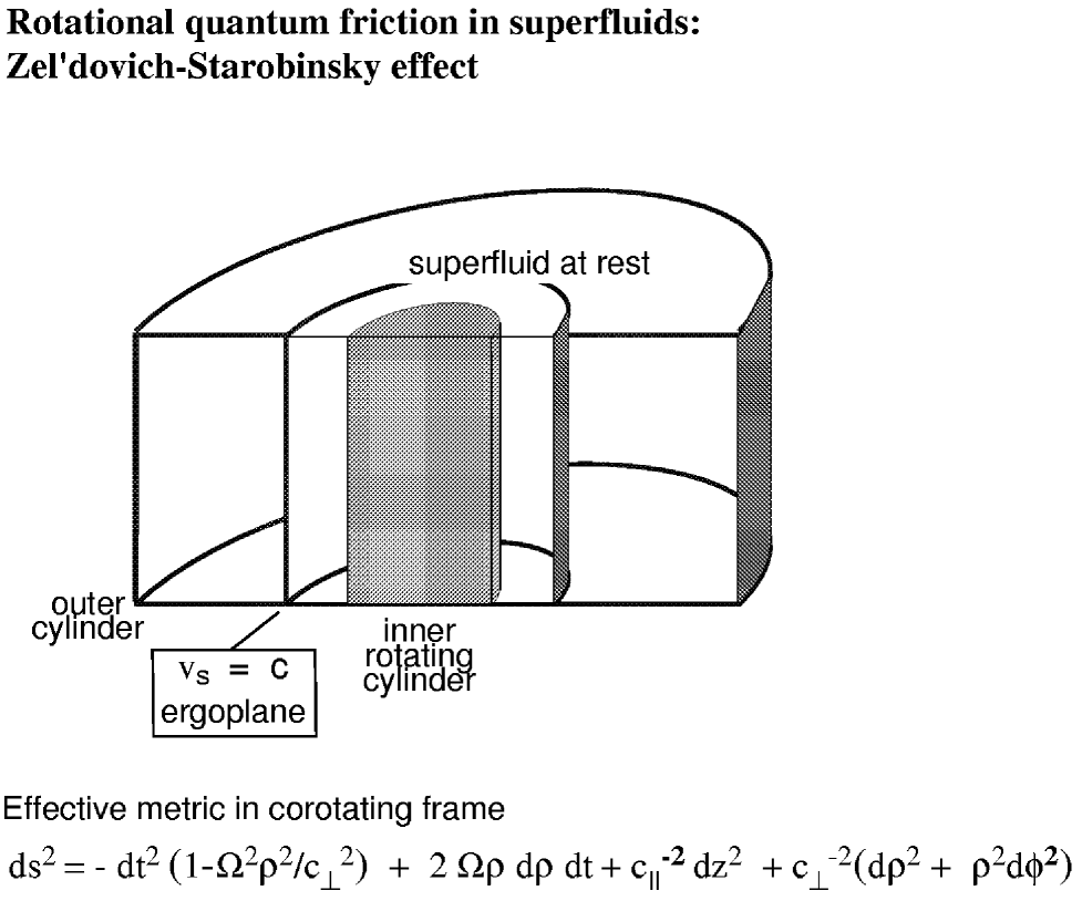
FIG. 25.: Possible simulation of Zel’dovich-Starobinsky effect in superfluids. The inner cylinder rotates forming the preferred rotating reference frame. In this frame the effective metric has an ergoregion, where the negative energy levels are empty.

The motion with constant angular velocity is another realization of the Unruh effect[194]. In Uruh effect a body moving in the vacuum with linear acceleration $a$ radiates the thermal spectrum of excitations with the Unruh temperature $T_{\rm U}=\hbar a/2\pi c$. On the other hand the observer comoving with the body sees the vacuum as a thermal bath with $T=T_{\rm U}$, so that the matter of the body gets heated to $T_{\rm U}$ (see references in [195]). It is difficult to simulate in condensed matter the motion at constant proper acceleration (hyperbolic motion). On the other hand the body rotating in superfluid vacuum simulates the uniform circular motion of the body with the constant centripetal acceleration. Such motion in the quantum vacuum was also heavily discussed in the literature (see the latest references in [196, 197, 198]). The latter motion is stationary in the rotating frame, which is thus a convenient frame for study of the radiation and thermalization effects for uniformly rotating body.

Zel’dovich [199] was the first who predicted that the rotating body (say, dielectric cylinder) amplifies those electromagnetic modes which satisfy the condition

$$\omega-L\Omega<0~{}.$$ (375)

Here $\omega$ is the frequency of the mode, $L$ is its azimuthal quantum number, and $\Omega$ is the angular velocity of the rotating cylinder. This amplification of the incoming radiation is referred to as superradiance [200]. The other aspect of this phenomenon is that due to quantum effects, the cylinder rotating in quantum vacuum spontaneously emits the electromagnetic modes satisfying Eq.(375) [199]. The same occurs for any rotating body, including the rotating black hole [201], if the above condition is satisfied.

Distinct from the linearly accelerated body, the radiation by a rotating body does not look thermal. Also, the rotating observer does not see the Minkowski vacuum as a thermal bath. This means that the matter of the body, though excited by interaction with the quantum fluctuations of the Minkowski vacuum, does not necessarily acquire an intrinsic temperature depending only on the angular velocity of rotation. Moreover the vacuum of the rotating frame is not well defined because of the ergoregion, which exists at the distance $r_{e}=c/\Omega$ from the axis of rotation.

Let us consider a cylinder of radius $R$ rotating with angular velocity $\Omega$ in the (infinite) superfluid liquid (Fig. 25). When the body rotates, the energy of quasiparticles is not well determined in the laboratory frame due to the time dependence of the potential, caused by the rotation of the body, whose surface is never perfect. The quasiparticle energy is well defined in the rotating frame, where the potential is stationary. Hence it is simpler to work in the rotating frame. If the body is rotating surrounded by the stationary superfluid, i.e. ${\bf v}_{\rm s}=0$ in the laboratory frame, then in the rotating frame one has ${\bf v}_{\rm s}=-{\bf\Omega}\times{\bf r}$. Substituting this ${\bf v}_{\rm s}=0$ in Eq.(37) one obtains that line element, which determines the propagation of phonons in the frame of the body, corresponds to the conventional metric of flat space in the rotating frame:

$$ds^{2}=-(c^{2}-\Omega^{2}\rho^{2})dt^{2}-2\Omega\rho^{2}d\phi dt+dz^{2}+\rho^{2}d\phi^{2}+d\rho^{2}~{}.$$ (376)

The azimuthal motion of the quasiparticles in the rotating frame can be quantized in terms of the angular momentum $L$, while the radial motion can be treated in the quasiclassical approximation. Then the energy spectrum of the phonons in the rotating frame is

$$\tilde{E}=E(p)+{\bf p}\cdot{\bf v}_{\rm s}=c\sqrt{{L^{2}\over\rho^{2}}+p_{z}^{2}+p_{\rho}^{2}}-\Omega L~{}.$$ (377)

For rotons and Bogoliubov fermions in ³He-B the energy spectrum in the rotating frame is

$$\tilde{E}(p)=\Delta+{(p-p_{0})^{2}\over 2m_{0}}-\Omega L~{},$$ (378)

$$\tilde{E}(p)=\sqrt{\Delta_{B}^{2}+v_{F}^{2}(p-p_{F})^{2}}-\Omega L~{},$$ (379)

where $p_{0}$ marks the roton minimum in superfluid ⁴He, while $\Delta$ is a roton gap.

2 Ergoregion in superfluids.

For the “relativistic” phonons the radius $\rho_{e}^{\rm rel}=c/\Omega$, where $g_{00}=0$, marks the position of the ergoplane. In the ergoregion, i.e. at $\rho>\rho_{e}^{\rm rel}=c/\Omega$, the energy of phonons in Eq.(377) can become negative for any rotation velocity and $\Omega L>0$ (Fig. 26). However, the real ergoplane in superfluid ⁴He occurs at $\rho_{e}=v_{\rm Landau}/\Omega$, where the Landau velocity in Eq.(343) is $v_{\rm Landau}\sim\Delta/p_{0}$. Let us assume that the angular velocity of rotation $\Omega$ is small enough, so that the linear velocity on the surface of the cylinder is much less than the Landau critical velocity $\Omega R<v_{\rm Landau}$. Thus excitations can never be nucleated at the surface of cylinder. However, in the ergoplane the velocity $v_{\rm s}=\Omega\rho_{e}$ in the rotating frame reaches $v_{\rm Landau}$, so that quasiparticle can be created in the ergoregion $\rho>\rho_{e}$.

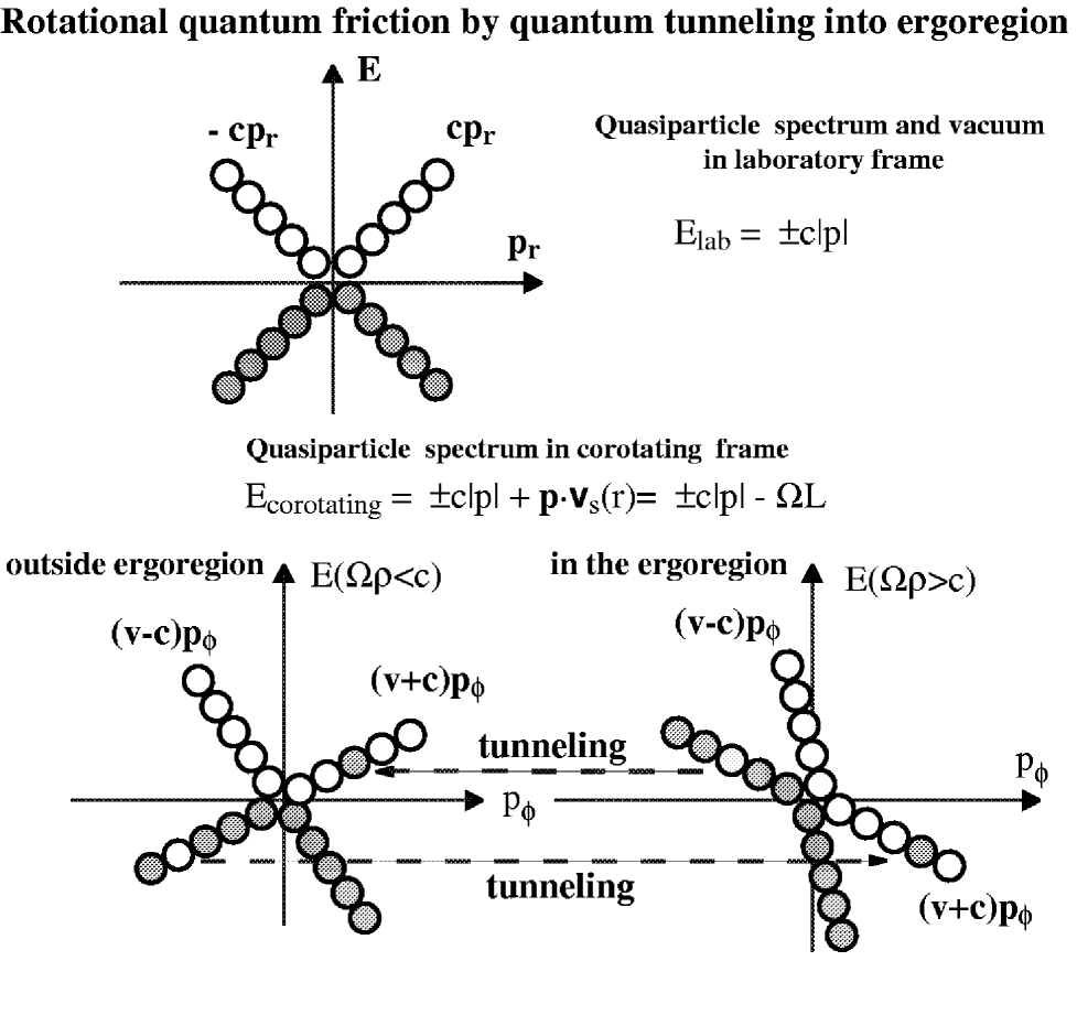
FIG. 26.: Vacuum seen in the frame corotating with inner cylinder is different from that viewed in the laboratory frame. The states which are occupied in the vacuum viewed in the laboratory frame are shaded. If the ergoplane is close to the rotating inner cylinder and is far from the outer cylinder, which is at rest in the laboratory frame, the influence of the rotating cylinder on the quasiparticle behavior is dominating. Thus the relevant frame for quasiparticles is the rotating frame. In the ergoregion, some states, which are occupied in the laboratory vacuum, have positive energy in the corotating frame. The quasiparticles occupying these levels must be radiated away. At $T=0$ the radiation occurs via quantum tunneling from or to the region in the vicinity of the surface of inner cylinder, where the interaction with the rotating cylinder occurs. The rate of tunneling reproduces the Zel’dovich-Starobinsky effect of radiation from the rotating black hole.

The process of creation of quasiparticles is determined by the interaction with the rotating body; there is no radiation in the absence of the body. If $\Omega R\ll v_{\rm Landau}=c$ one has $\rho_{e}\gg R$, i.e. the ergoregion is situated far from the cylinder; thus the interaction of the phonons state in the ergoregion with the rotating body is small. This results in a small emission rate and thus in a small value of quantum friction, as will be discussed below.

In superfluid ⁴He the Landau velocity for the emission of rotons is smaller than that for the emission of phonons, $v_{L}=c$. That is why the ergoplane for rotons, $\rho_{e}=v_{\rm Landau}/\Omega$, is closer to the cylinder, than the plane $\rho_{e}^{\rm rel}=c/\Omega$. However, it appears (see below) that the emission of the rotons is exponentially suppressed due to the big value of the allowed angular momentum for emitted rotons: the Zel’dovich condition Eq.(375) for roton spectrum is satified only for $L>\Delta/\Omega\gg 1$.

3 Radiation to the ergoregion as a source of rotational quantum friction.

For the Bose case the radiation of quasiparticles can be also considered as the process in which the particle in the normal Bose liquid in the surface layer near surface of the rotating cylinder tunnels to the scattering state at the ergoplane, where its energy is also $\tilde{E}=0$ (Fig. 26). In the quasiclassical approximation the tunneling probability is $e^{-2S}$, where

$$S={\rm{Im}}\int d\rho~{}p_{\rho}(\tilde{E}=0)~{}.$$ (380)

For the phonons with $p_{z}=0$ one has

$$S=L\int^{\rho_{e}}_{R}d\rho~{}\sqrt{{1\over\rho^{2}}-{1\over\rho_{e}^{2}}}\approx L\ln{\rho_{e}\over R}~{}.$$ (381)

Thus all the phonons with $L>0$ are radiated, but the radiation probability decreases at higher $L$. If the linear velocity at the surface is much less than $c$, i.e. $\Omega R\ll c$, the probability of radiation of phonons with the energy (frequency) $\omega=\Omega L$ becomes

$$w\propto e^{-2S}=\left({R\over\rho_{e}}\right)^{2L}=\left({\Omega R\over c}\right)^{2L}=\left({\omega R\over cL}\right)^{2L}~{},~{}\Omega R\ll c~{}.$$ (382)

If $c$ is substituted by the speed of light, Eq.(382) is proportional to the superradiant amplification of the electromagnetic waves by rotating dielectric cylinder derived by Zel’dovich [200, 202].

The number of phonons with the frequency $\omega=\Omega L$ emitted per unit time can be estimated as $\dot{N}=We^{-2S}$, where $W$ is the attempt frequency $\sim\hbar/ma^{2}$ multiplied by the number of localized modes $\sim RZ/a^{2}$, where $Z$ is the height of the cylinder. Since each phonon carries the angular momentum $L$, the cylinder rotating in superfluid vacuum (at $T=0$) is loosing its angular momentum, which means the quantum rotational friction.

Let us consider the same process for the rotons. The minimal $L$ value of the radiated quasiparticles, which have the gap $\Delta$, is determined by this gap: $L_{min}=\Delta/\Omega p_{0}=v_{\rm Landau}/\Omega$, where $v_{\rm Landau}=\Delta/p_{0}$ is the Landau critical velocity for emission of rotons. Since the tunneling rate exponentially decreases with $L$, only the lowest possible $L$ must be considered. In this case the tunneling trajectory with $E=0$ is determined by the equation $p=p_{0}$ both for rotons and Bogoliubov quaiparticles. For $p_{z}=0$ the classical tunneling trajectory is thus given by $p_{\rho}=i\sqrt{|p_{0}^{2}-L^{2}/\rho^{2}|}$. This gives for the tunneling exponent $e^{-2S}$ the equation

$$S={\rm{Im}}\int d\rho~{}p_{\rho}=L\int^{\rho_{e}}_{R}dr~{}\sqrt{{1\over\rho^{2}}-{1\over\rho_{e}^{2}}}\approx L\ln{\rho_{e}\over R}~{}.$$ (383)

Here the position of the ergoplane is $\rho_{e}=L/p_{0}=v_{\rm Landau}/\Omega$. Since the rotation velocity $\Omega$ is always much smaller than the gap, $L$ is very big. That is why the radiation of rotons and Bogoliubov quasiparticles with the gap is exponentially suppressed.

XIV How to improve helium-3.

A Gradient expansion

Though ³He-A and Standard Model belong to the same universality class and thus they have similar properties of the fermionic spectrum, the ³He-A cannot serve as a good model for quantum vacuum. The effective action for bosonic gauge and gravity fields obtained by integration over fermionic degrees of freedom is contaminated by the terms which are absent in a fully relativistic system. This is because the integration over fermions is not always concentrated in the region where their spectrum is “relativistic”. Thus the question arises whether we can “correct” the ³He-A in such a way that these uncomfortable terms are suppressed.

If we neglect the spin degrees of freedom, the massless bosonic fields which appear in ³He-A due to the breaking of symmetry $U(1)_{N}\times SO(3)_{L}$ is the triad field, which can be expressed in terms of the superfluid velocity (torsion) and the $\hat{\bf l}$-field. The quadratic energy in terms of the gradients of the soft Goldstone variables (the London energy for ³He-A) in the reference frame where the heat bath is at rest, ${\bf v}_{\rm n}=0$, can be written in the following general form [13]:

$$F_{\rm London}={m\over 2}n_{{\rm s}\parallel}\left(\hat{\bf l}\cdot{\bf v}_{\rm s}\right)^{2}+{m\over 2}n_{{\rm s}\perp}\left(\hat{\bf l}\times{\bf v}_{\rm s}\right)^{2}$$ (384)

$$+{1\over 2}\left(C(\hat{\bf l}\times{\bf v}_{\rm s})\cdot(\hat{\bf l}\times(\nabla\times\hat{\bf l}))-(C_{0}-C)(\hat{\bf l}\cdot{\bf v}_{\rm s})(\hat{\bf l}\cdot(\nabla\times\hat{\bf l}))\right)$$ (385)

$$+(K_{s}(\nabla\cdot\hat{\bf l})^{2}+K_{t}(\hat{\bf l}\cdot(\nabla\times\hat{\bf l}))^{2}+K_{b}(\hat{\bf l}\times(\nabla\times\hat{\bf l}))^{2}$$ (386)

The temperatutre dependent coefficients can be obtained within the framework of the BCS theory if one applies the gradient expansion [203]. In its simplest form of BCS theory the gradient energy is determined by 4 parameters:

The ‘speeds of light” $c_{\parallel}=v_{F}$ and $c_{\perp}$ characterize the “relativistic” physics of the low-energy corner. These are the parameters of the quasiparticles in the “relativistic” low-energy corner below the first “Planck scale”, $E\ll\Delta_{0}^{2}/v_{F}p_{F}$.

The parameter $p_{F}$ is the property of the higher level in the hierarchy of the energy scales – the Fermi-liquid level. The related quantity is the quasiparticle mass in the Fermi-liquid theory, $m^{*}=p_{F}/c_{\parallel}$. This parameter also determined the second “Planck” energy scale $\Delta_{0}=p_{F}c_{\perp}$. The spectrum of quasiparticles in ³He-A in the whole range $E\ll v_{F}p_{F}$ is determined by these 3 parameters, $c_{\parallel}$, $c_{\perp}$ and $p_{F}$.

Finally the bare mass $m$ of ³He is the parameter of the underlying microscopic physics of interacting “indivisible” particles – ³He atoms. This parameter does not enter the spectrum of quasiparticles in ³He-A and thus the naive BCS theory. However the Galilean invariance of the underlying system of ³He atoms requires that the kinetic energy of superflow at $T=0$ must be $(1/2)mn{\bf v}_{\rm s}^{2}$, i.e. the bare mass $m$ must be incorporated into the BCS scheme to maintain the Galilean invariance. This is achieved in the Landau theory of Fermi liquid, where the dressing occurs due to quasiparticles interaction. In the simplified approach one can consider only that part of interaction which is responsible for the renormalization of the mass and which restores the Galilean invariance of the Fermi system. This is the current-current interaction with the Landau parameter $F_{1}=3(m^{*}/m-1)$, containg the bare mass $m$. This is the way how the bare mass $m$ enters the Fermi-liquid and thus the BCS theory.

In the real ³He liquid the ratio $m^{*}/m$ varies between about 3 and 6 depending on pressure. However, in the modified BCS theory this ratio can be considered as a free parameter, which one can ajust to make the system more close to the relativistic theories. As we discussed in Sec. II H, the superfluidity must be suppressed for the correct Einstein term to prevail in the effective action for gravity. This must happen if $m\rightarrow\infty$. In this limit the superfluid properties of the liquid are really suppressed, since the superfluid velocity is inversly proportional to $m$ according to Eq. (100), ${\bf v}_{\rm s}\propto 1/m$. In this limit of heavy mass of atoms comprising the vacuum, the vacuum becomes inert, and the kinetic energy of superflow $(1/2)mn{\bf v}_{\rm s}^{2}$, which is dominating over the Einstein action in real ³He-A, vanishes as $1/m$. Thus we can expect that in case of inert vacuum, the influence of the microscopic level on the effective theory of gauge field and gravity is suppressed and the effective action for the collective modes approaches the covariant and gauge invariant limit of the Einstein-Maxwell action.

For illustration that this really happens, let us consider how all these 4 parameters enter the gradient energy in Eq.(384-386) and what happens when $m\rightarrow\infty$. According to Cross [203] one has the following expression for the coefficients in the gradient expansion (we are interested in a low-temperature region $T\ll\Delta_{0}$). The normal (and thus superfluid) component densities are given by Eq.(10), which for the ³He-A quasiparticles are

$$n_{{\rm n}\parallel}\approx{m^{*}\over m}n^{0}_{{\rm n}\parallel}~{},~{}n^{0}_{{\rm n}\parallel}=\pi^{2}n{T^{2}\over\Delta_{0}^{2}}~{},~{}n_{{\rm s}\parallel}=n-n_{{\rm n}\parallel}~{},~{}n^{0}_{{\rm s}\parallel}=n-n^{0}_{{\rm n}\parallel}~{},$$ (387)

$$n_{{\rm n}\perp}={m^{*}\over m}n^{0}_{{\rm n}\perp}~{},~{}n^{0}_{{\rm n}\perp}={7\pi^{4}\over 15}n{T^{4}\over\Delta_{0}^{4}}~{},~{}n_{{\rm s}\perp}=n-n_{{\rm n}\perp}~{},~{}n^{0}_{{\rm s}\perp}=n-n^{0}_{{\rm n}\perp}~{}.$$ (388)

Here we introduced (with index $0$) the bare (nonrenormalized) values of the normal and superfluid component densities, which correspond to the limit of noninteracting Fermi-gas with $F_{1}=0$ and thus to $m^{*}=m$. In the derivation we considered the low-temperature limit $T\ll\Delta_{0}$; also the small terms of order of the anisotropy parameter $c_{\perp}^{2}/c_{\parallel}^{2}\sim 10^{-6}$ have been neglected, so that the particle density is the same in normal and superfluid states: $n={p_{F}^{3}\over 3\pi^{2}}$. The other parameters are accoring to [203]

$$C_{0}-C={1\over 2m}n_{{\rm s}\parallel}~{},~{}C={1\over 2m}n_{{\rm s}\perp}{n^{0}_{{\rm s}\parallel}\over n^{0}_{{\rm s}\perp}}~{},$$ (389)

$$K_{s}={1\over 32m^{*}}n^{0}_{{\rm s}\perp}~{},$$ (390)

$$K_{t}={1\over 96m^{*}}\left(n^{0}_{{\rm s}\perp}+4n^{0}_{{\rm s}\parallel}+3\left({m^{*}\over m}-1\right){n_{{\rm s}\parallel}n^{0}_{{\rm s}\parallel}\over n}\right)~{}$$ (391)

$$K_{b}={1\over 32m^{*}}\left(2n^{0}_{{\rm s}\parallel}+\left({m^{*}\over m}-1\right){n_{{\rm s}\parallel}n^{0}_{{\rm s}\parallel}\over n}\right)+{\rm Log}~{},$$ (392)

$$~{}{\rm Log}={1\over 4m^{*}}n\int{d\Omega\over 4\pi}{(\hat{\bf l}\cdot\hat{\bf p})^{4}\over(\hat{\bf l}\times\hat{\bf p})^{2}}\left[1+2\int_{0}^{\infty}dM{\partial f_{\cal T}\over\partial E}\right]~{}.$$ (393)

Here ${\rm Log}$ is the term which contains $\ln(\Delta_{0}/T)$. The integral in Eq.(393) is over the solid angle in momentum space; the energy spectrum which enters the equilibrium quasiparticle distribution function $f_{\cal T}=(1+\exp{E/T})^{-1}$, with $E^{2}=M^{2}+\Delta_{0}^{2}(\hat{\bf p}\times\hat{\bf l})^{2}$ as is given by Eq.(96). This coefficient does not depend on the microscopic parameter $m$ and represents the logarithmically diverging coupling constant in the Maxwell effective action for the magnetic field in curved space in Eq.(124).

B Effective action in inert vacuum.

In the limit $m\rightarrow\infty$ all the terms related to superfluidity vanish since $v_{s}\propto 1/m$. Taking into account that in this limit $n_{s\parallel}=n$ one obtains for the remaining ${\hat{\bf l}}$-terms:

$$F_{\rm London}(m\rightarrow\infty)={1\over 32m^{*}}n^{0}_{s\perp}(\nabla\cdot\hat{\bf l})^{2}+{1\over 96m^{*}}(n^{0}_{s\perp}+n^{0}_{s\parallel})(\hat{\bf l}\cdot(\nabla\times\hat{\bf l}))^{2}+\left({1\over 32m^{*}}n^{0}_{s\parallel}+{\rm Log}\right)(\hat{\bf l}\times(\nabla\times\hat{\bf l}))^{2}~{}.$$ (394)

All three terms have the correspondence in QED and Einstein gravity. We have already seen that the bend term, i.e. $(\hat{\bf l}\times(\nabla\times\hat{\bf l}))^{2}$, is exactly the energy of the the magnetic field in curved space with the logarithmically diverging coupling constant. Let us now consider the twist term, i.e. $(\hat{\bf l}\cdot(\nabla\times\hat{\bf l}))^{2}$ and show that it corresponds to the Einstein action.

1 Einstein action in ³He-A.

The part of effective gravity, which is simulated by the superfluid velocity field, vanishes in the limit of inert vacuum. The remaining part of gravitational field is simulated by the inhomogeneity of the $\hat{\bf l}$ field, which plays the part of the “Kasner axis” in the metric

$$g^{ij}=c_{\parallel}^{2}\hat{l}^{i}\hat{l}^{j}+c_{\perp}^{2}(\delta^{ij}-\hat{l}^{i}\hat{l}^{j})~{},~{}g^{00}=-1,~{}g^{0i}=0,~{}\sqrt{-g}={1\over c_{\parallel}c_{\perp}^{2}},$$ (395)

$$g_{ij}={1\over c_{\parallel}^{2}}\hat{l}^{i}\hat{l}^{j}+{1\over c_{\perp}^{2}}(\delta^{ij}-\hat{l}^{i}\hat{l}^{j}),~{}g^{00}=-1~{},~{}g^{0i}=0~{}.$$ (396)

The curvature of the space with this metric is caused by spatial rotation of the “Kasner axis” $\hat{\bf l}$. For the stationary metric, $\partial_{t}\hat{\bf l}=0$, one obtains that in terms of the $\hat{\bf l}$-field the Einstein action is

$$-{1\over 16\pi G}\int\sqrt{-g}R={1\over 32\pi G\Delta_{0}^{2}}\left(1-{c_{\perp}^{2}\over c_{\parallel}^{2}}\right)^{2}{p_{F}^{3}\over m^{*}}\int((\hat{\bf l}\cdot(\nabla\times\hat{\bf l}))^{2}~{}.$$ (397)

It has the structure of the twist term in the gradient energy (394) obtained in gradient expansion, which in the inert vacuum limit is

$$F_{\rm twist}={1\over 288}\left({2\over\pi^{2}}-{T^{2}\over\Delta_{0}^{2}}\right){p_{F}^{3}\over m^{*}}\int((\hat{\bf l}\cdot(\nabla\times\hat{\bf l}))^{2}$$ (398)

We thus can identify the twist term with Einstein action. Neglecting the small anisotropy factor ${c_{\perp}^{2}\over c_{\parallel}^{2}}$ one obtains that the Newton constant in the effective gravity of the “improved” ³He-A is:

$$G^{-1}={2\over 9\pi}\Delta_{0}^{2}-{\pi\over 9}T^{2}~{}.$$ (399)

While the temperature independent part certainly depends on the details of the transPlanckian physics, the temperature dependence of the Newton constant pretends to be universal, since it does not depend on the parameters of the system. If one applies the regularization scheme provided by the transPlanckian physics of ³He to the relativistic system one would suggest the following temperature dependence of Newton constant in the vacuum with $N_{F}$ Weyl fermions ($N_{F}=2$ for ³He-A):

$$\delta[G^{-1}]=-{\pi\over 18}N_{F}T^{2}~{}.$$ (400)

2 Violation of gauge invariance.

Let us finally consider the splay term $(\nabla\cdot\hat{\bf l})^{2}$ in Eq.(394). It has only the 4-th order temperature corrections, $T^{4}/\Delta_{0}^{4}$. This term has similar coefficient as the curvature term, but it is not contained in Einstein action, since it cannot be written in the covariant form. The structure of this term can be, however, obtained using the gauge field presentation of the $\hat{\bf l}$ vector, where ${\bf A}=p_{F}\hat{\bf l}$. It is known that similar term can be obtained in the renormalization of QED in the leading order of $1/N$ theory if the regularization is made by introducing the momentum cut-off: [204]:

$$L^{\prime}_{QED}={1\over 96\pi^{2}}(\partial_{\mu}A_{\mu})^{2}~{}.$$ (401)

This term violates the gauge invariance and does not appear in the dimensional regularization scheme [205], but it appears in the momentum cut-of procedure, which violates the gauge invariance. Being written in covariant form the Eq.(401) can be applied to ³He-A, where ${\bf A}=p_{F}\hat{\bf l}$ and $\sqrt{-g}=Const$:

$$L^{\prime}_{QED}={1\over 96\pi^{2}}\sqrt{-g}(\partial_{\mu}(g^{\mu\nu}A_{\nu}))^{2}=~{}{1\over 96\pi^{2}}{p_{F}^{2}c_{\parallel}^{3}\over c_{\perp}^{2}}(\nabla\cdot\hat{\bf l})^{2}={c_{\parallel}^{2}\over c_{\perp}^{2}}{1\over 96\pi^{2}}{p_{F}^{3}\over m^{*}}(\nabla\cdot\hat{\bf l})^{2}.$$ (402)

This term corresponds to the splay term in Eq.(394), but it contains an extra big factor of the vacuum anisotropy $c_{\parallel}^{2}/c_{\perp}^{2}$: $F_{London~{}splay}=(c_{\perp}^{2}/c_{\parallel}^{2})L^{\prime}_{QED}$. However, in the isotropic case, where $c_{\parallel}=c_{\perp}$, they exactly coincide. This suggests that the regularization provided by the “transPlanckian physics” of ³He-A represents the anisotropic version of the momentum cut-off regularization of quantum electrodynamics.

XV Discussion

Let us summarize the parallels between the quantum vacuum and superfluids, which were touched upon in the review, and their possible influence on the quantum field theory.

Superfluid ³He-A and other possible representative of its universality class provides an example of how the chirality, Weyl fermions, gauge fields and gravity can emergently appear in the low emergy corner together with the corresponding symmetries, which include the Lorentz symmetry and local $SU(N)$ symmetry. This supports the “anti-grand-unification” idea that the quantum field theory, such as Standard Model or maybe GUT, is an effective theory, which is applicable only in the infrared limit. Most of the symmetries of this effective theory are the attributes of the theory: the symmetries gradually appear in the low-energy corner together with the effective theory itself.

The momentum space topology of the fermionic vacuum (Sec. IV) is instrumental in determination of the universality class of the system. It provides the topological stability of the low-energy properties of the systems of given class: the character of the fermionc spectrum, collective modes and leading symmetries. The universality class, which contains topologically stable Fermi points, is common for superfluid ³He-A and Standard Model. This allowed us to provide analogies between many phenomena in the two systems, which have the same physics but in many cases are expressed in different languages and can be visualized in terms of different observables. However, in the low-energy corner they are described by the same equations if they are written in the covariant and gauge invariant form. On this topological ground it appears that some of the unification schemes of the strong and electroweak interactions is more preferrable than the others: this is the $SU(4)_{C}\times SU(2)_{L}\times SU(2)_{R}$ group (Sec. V B).

The advantage of ³He-A is that this system is complete being described by the BCS model. This scheme incorporates not only the “relativistic” infrared regime, but also several successive scales of the short-distance physics, which correspond to different ultraviolet “transPlanckian” ranges of high energy. Since in BCS scheme there is no need for a cut-off imposed by hand, all subtle issues of the cut-off in quantum field theory can be resolved on physical grounds. It appears, however, the ³He-A is not a perfect object for the realization of the completely covariant effective gauge and gravity fields at low energy, because the effect of the “transPlanckian” physics shows up even in the low-energy corner. This in particular leads to many noncovariant terms in the effective action, including the mass of the graviton. On the other hand, it is clear how to “correct” the ³He-A: the Lorentz invariance must be extended far into the “transPlanckian” region to kill the noncovariant non-renormalizable terms. The killing is however never complete, the “nonrenormalizable” terms are always there in effective theory though they are small since contain the Planck energy cut-off $E_{\rm P}$ in denominator. One example of such “nonrenormalizable” term in ³He-A, which is the remnant of the “transPlanckian” physics, corresponds to the mass term for the $U(1)_{Y}$ gauge field of the hyperphoton which violates the gauge invariance (Sec. VIII B 4).

Thus the condensed matter of the Fermi-point universality class shows one of possibly many routes from the low-energy “relativistic” to high energy “transPlanckian” physics. Of course, one might expect the many routes to high energy, since the systems of the same universality class become similar only in the vicinity of the fixed point: they can diverge far from each other at higher energies. Nevertheless, probably the first corrections could be similar too.

Practically in all condensed matters of even different universality classes, the effective action for some bosonic or even fermionic modes acquires an effective Lorentzian metric. That is why the gravity is the field, which can be simulated most easily in condensed matter. The gravity can be simulated by flowing normal fluids, superfluids, and Bose-Einstein condensates; by elastic strains, disclocations and disclinations in crystals, etc. Though the full dynamical realization of gravity takes place only in the fermionic condensed matter with Fermi points, the acoustic type of gravity are also useful for simulation of different phenomena related to marriage of gravity and quantum theory.

The analog of gravity in superfluids shows the possible way how to solve the cosmological constant problem. The standard calculations of the energy density of superfluid ground state in the framework of the effective theory suggests that it is of the order of $E_{\rm P}^{4}$, if one translates it into the language of the relativistic theories. It is of the same magnitude as the field theoretical estimation for the vacuum energy and thus for the cosmological constant. However, the stability analysis of the ground state of the isolated superfluid liquid, which is certainly beyond the effective theory, strongly forces the exact nullification of the appropriate energy density of the liquid, which enters the Lagrangian at $T=0$ (Sec. II G). In terms of the relativistic quantum field theory this means that the equilibrium vacuum should not gravitate. And this conclusion cannot be obtained from the effective theory, while in the underlying microscopic physics this result of the complete nullification does not depend on the microscopic details. It is universal in terms of the transPlanckian physics, but not in terms of the effective theory.

But what happens if the phase transition occurs in which the symmetry of the vacuum is broken, as is supposed to happen in early Universe when, say, the electroweak symmetry was broken? In the effectve theory, such transition must be accompanied by the change of the vacuum energy, which means that the vacuum has a huge energy either above or below the transition. However, in exact microscopic theory of liquid the phase transition does not disturb the zero value of the vacuum energy (Sec. X C), if the liquid remains in equilibrium. The energy change is completely compensated by the change of the chemical potential of the underlying atoms of the liquid which comprise the vacuum state – the quantity which is not known in effective theory. Moreover, the analogy with the superfluids also shows that in nonequilibrium case or at nonzero $T$ (Secs. III F and X C) the effective vacuum energy must be of order of the energy density of matter. This is in agreement with the mordern astrophysical observations.

Another object, where as in the problem of gravitating vacuum the marriage of gravity and quantum theory is important, is the black hole. Having many objects for simulation of gravity, we can expect in the nearest future that the analogs of event horizon could be constructed in the laboratory. Most probably this will first happen in the laser trapped Bose condensates [206]. The condensed matter analogs of horizons may exhibit Hawking radiation, but in addition the other, unexpected, effects related to quantum vacuum could arise, such as instability experienced by vacuum in the acoustic model of gravity. Because the short-distance physics is explicitly known in condensed matter this helps clarify the problem related to the vacuum in the presence of the horizon, or in the other exotic effective metric, such as the degenerate metric (Sec. XI A).

At the moment only one of the exotic metrics has been experimentally simulated. This is the metric induced by spinning cosmic string, which produces the analog of the gravitational Aharonov-Bohm effect, experienced by particles in the presence of such string. This type of Aharonov-Bohm effect has been experimentally confirmed in superfluids by measurement of the Iordanskii force acting on quantized vortices (Sec. XII).

As for the other (nongravitational) analogies, the most interesting are related to the interplay between the vacuum and the matter, and which can be fully investigated in condensed matter, because of the absence of the cut-off problem. These are the anomalies, which are at the origin of the exchange of the fermionic charges between the vacuum and the matter. Such anomalies are the attributes of the Fermi systems of universality class of Fermi points: Standard Model and ³He-A. The spectral flow from the vacuum to the matter, which carries the fermionic charge from the vacuum to matter, occurs just through the Fermi point. Since in the vicinity of the Fermi point the equations are the same for the two Fermi systems, the spectral flow in both systems is described by the same Adler, and Bell and Jackiw equation for axial anomaly [74, 75] (Sec. VII). The ³He-A provided the first experimental prove for the anomalous nucleation of the fermionic charge from the vacuum. The Adler-Bell-Jackiw equation was confirmed up to the numerical value of the factor $1/4\pi^{2}$ with the precision of few percent. The anomalous nucleation of the baryonic or leptonic charge is in the basis of the modern theories of the baryogenesis.

The modified equation is obtained for the nucleation of the fermionic charge by the moving string – the quantized vortex. The transfer of the fermionic charge from the “vacuum” to “matter” is mediated by the fermion zero modes living on vortices. This condesed matter illustration of the cancellation of anomalies in 1+1 and 3+1 systems (the Callan-Harvey effect) has been experimentally verified in ³He-B. This also means that the scenario of the baryogenesis by cosmic strings has been experimentally probed. The other effect related to axial anomaly – the helical instability of the superfluid/normal counterflow in ³He-A – is also described by the same physics and by the same equations as the formation of the (hyper) magnetic field due to the helical instability experienced by the vacuum in the presence of the heat bath of the right-handed electrons (Sec. VIII C). That is why its experimental observation in ³He-A provided an experimental support for the Joyce-Shaposhnikov scenario of the genesis of the primordial magnetic field. In a future the macroscopic parity violating effect suggested by Vilenkin [97] must be simulated in ³He-A (Sec. VIII D). In both systems it is desribed by the same mixed axial-gravitational Chern-Simons action.

One may expect that the further theoretical and experimental exploration of the vacuum / condensed matter analogies will clarify the properties of the quantum vacuum.

REFERENCES

- [1] C.D. Frogatt and H.B. Nielsen, Origin of Symmetry, World Scientific, Singapore - New Jersey - London - Hong Kong, 1991.
- [2] S. Chadha, and H.B. Nielsen, Lorentz Invariance as a Low-Energy Phenomenon, Nucl. Phys. B 217, 125–144 (1983).
- [3] S. Weinberg, What is quantum field theory, and what did we think it is? hep-th/9702027
- [4] F. Jegerlehner, The “ether-world” and elementary particles, hep-th/9803021.
- [5] G.E. Volovik, Field theory in superfluid 3He: What are the lessons for particle physics, gravity and high-temperature superconductivity?, Proc. Natl. Acad. Sci. USA 96, 6042 - 6047 (1999), cond-mat/9812381,; G.E. Volovik, 3He and Universe parallelism, in “Topological Defects and the Non-Equilibrium Dynamics of Symmetry Breaking Phase Transitions”, Yu. M. Bunkov, H. Godfrin (Eds.), pp. 353-387 (Kluwer, 2000), cond-mat/9902171.
- [6] C. Rovelli, Notes for a brief history of quantum gravity, gr-qc/0006061.
- [7] R.B. Laughlin and D. Pines, The Theory of Everything, Proc. Natl. Acad. Sc. USA 97, 28-31 (2000).
- [8] B.L. Hu, Expanded version of an invited talk at 2nd International Sakharov Conference on Physics, Moscow, 20 - 23 May 1996, e-Print Archive: gr-qc/9607070.
- [9] T. Padmanabhan, Conceptual issues in combining general relativity and quantum theory, hep-th/9812018.
- [10] G.E. Volovik, Axial anomaly in 3He-A: Simulation of baryogenesis and generation of primordial magnetic field in Manchester and Helsinki, Physica B 255, 86 – 107 (1998).
- [11] I.M. Khalatnikov: An Introduction to the Theory of Superfluidity, (Benjamin, New York, 1965).
- [12] I.E. Dzyaloshinskii and G.E. Volovick, Poisson brackets in condensed matter, Ann. Phys. 125, 67 - 97 (1980); G.E. Volovik, Wess-Zumino action for the orbital dynamics of ,” JETP Lett. 44, 185 - 189 (1986); Linear momentum in ferromagnets, J. Phys. C 20, L83 - L87 (1987).
- [13] D. Vollhardt, and P. Wölfle, The superfluid phases of helium 3, Taylor and Francis, London - New York - Philadelphia, 1990.
- [14] W. G. Unruh, Experimental black-hole evaporation?, Phys. Rev. Lett. 46, 1351-1354 (1981); Sonic analogue of black holes and the effects of high frequencies on black hole evaporation, Phys. Rev. D 51, 2827-2838 (1995).
- [15] M. Visser, Acoustic black holes: horizons, ergospheres, and Hawking radiation, Class. Quantum Grav. 15, 1767-1791 (1998)
- [16] M. Stone, Iordanskii force and the gravitational Aharonov-Bohm effect for a moving vortex, Phys. Rev. B 61, 11780 – 11786 (2000).
- [17] M. Visser, Lorentzian Wormholes. From Einstein to Hawking, AIP Press, Woodbury, New York, 1995.
- [18] C.W. Woo, Microscopic calculations for condensed phases of helium, in: The Physics of Liquid and Solid Helium, Part I, eds. K.H. Bennemann and J.B. Ketterson (John Wiley & Sons, New York, 1976).
- [19] S. Weinberg, Rev. Mod. Phys. 61, 1 (1989).
- [20] A.G. Riess, A.V. Filippenko, M.C. Liu, P. Challis, A. Clocchiatti, A. Diercks, P.M. Garnavich, C.J. Hogan, S. Jha, R.P. Kirshner, B. Leibundgut, M. M. Phillips, D. Reiss, B.P. Schmidt, R.A. Schommer, R.C. Smith, J. Spyromilio, C. Stubbs, N.B. Suntzeff, J. Tonry, P. Woudt, R.J. Brunner, A. Dey, R. Gal, J. Graham, J. Larkin, S.C. Odewahn, and B. Oppenheimer, Tests of the accelerating universe with near-infrared observations of a high-redshift type Ia supernova, astro-ph/0001384.
- [21] A. D. Sakharov: Vacuum Quantum Fluctuations in Curved Space and the Theory of Gravitation, Dokl. Akad. Nauk 177, 70-71 (1967) [Sov. Phys. Dokl. 12, 1040-41 (1968)]
- [22] V. Frolov and D. Fursaev, Thermal fields, entropy, and black holes, Class. Quant. Grav. 15, 2041-2074 (1998).
- [23] L.D. Landau and E.M. Lifshitz, Classical Fields, Pergamon Press, Oxford, 1975.
- [24] R.C. Tolman: Relativity, Thermodynamics and Cosmology (Clarendon Press, Oxford, 1934).
- [25] G.E. Volovik and V.P. Mineev, Current in superfluid Fermi liquids and the vortex core structure, Sov. Phys. JETP 56, 579 - 586 (1982).
- [26] P.G. Grinevich and G.E. Volovik, Topology of gap nodes in superfluid 3He, J. Low Temp. Phys. 72, 371-380 (1988).
- [27] J.M. Luttinger, Phys. Rev. 119, 1153 (1960).
- [28] M. Oshikawa, Topological Approach to Luttinger’s Theorem and the Fermi Surface of a Kondo Lattice, Phys. Rev. Lett. 84, 3370-3373 (2000).
- [29] G.E. Volovik, A new class of normal Fermi liquids, JETP Lett. 53, 222-225 (1991).
- [30] K.B. Blagoev and K.S. Bedell, Luttinger theorem in one dimensional metals, Phys. Rev. Lett. 79, 1106-1109 (1997).
- [31] Wen, X.G. (1990) Metallic non-Fermi-LiquidFermi liquid Fixed Point in Two and Higher Dimensions, Phys. Rev. B 42, 6623-6630.
- [32] H.J. Schulz, G. Cuniberti, and P. Pieri, Fermi liquids and Luttinger liquids, cond-mat/9807366.
- [33] V.M. Yakovenko, Metals in a high magnetic field: a universality class of marginal Fermi liquid, Phys. Rev. B 47, 8851-8857 (1993).
- [34] Y. Nambu and G. Jona-Lasinio, Dynamical model of elementary particles based on an analogy with superconductivity. I., Phys. Rev. 122, 345-358 (1961); Dynamical model of elementary particles based on an analogy with superconductivityİI., Phys. Rev. 124, 246-254 (1961).
- [35] M. Alford, K. Rajagopal and F. Wilczek, QCD at Finite Baryon Density: Nucleon Droplets and Color Superconductivity, Phys. Lett. B 422, 247-256 (1998);F. Wilczek, F. From Notes to Chords in QCD, Nucl. Phys. A 642, 1-13 (1998).
- [36] V.M.H. Ruutu, V.B. Eltsov, A.J. Gill, T.W.B. Kibble, M. Krusius, Yu.G. Makhlin, B. Placais, G.E. Volovik and Wen Xu, Vortex formation in neutron-irradiated superfluid 3He as an analogue of cosmological defect formation, Nature 382, 334–336 (1996) .
- [37] T.W.B. Kibble, Topology of cosmic domains and strings, J. Phys. A 9, 1387–1398 (1976) .
- [38] T.D.C. Bevan, A.J. Manninen, J.B. Cook, J.R. Hook, H.E. Hall, T. Vachaspati and G.E. Volovik, Momentogenesis by 3He vortices: an experimental analogue of primordial baryogenesis, Nature, 386, 689-692 (1997).
- [39] H.B. Nielsen and M. Ninomiya, Absence of neutrinos on a lattice. I - Proof by homotopy theory, Nucl. Phys. B 185, 20 (1981), [Erratum - Nucl. Phys. B 195, 541 (1982)]; Nucl. Phys. B 193 173 (1981).
- [40] G. E. Volovik, Exotic properties of superfluid 3He, World Scientific, Singapore - New Jersey - London - Hong Kong, 1992.
- [41] G.E. Volovik, and V.M. Yakovenko, Fractional charge, spin and statistics of solitons in superfluid 3He film, J. Phys.: Cond. Matter 1, 5263-5274 (1989).
- [42] G. E. Volovik, On edge states in superconductor with time inversion symmetry breaking, JETP Lett. 66 , 522-527 (1997).
- [43] K. Ishikawa, and T. Matsuyama, Z. Phys. C 33, 41 (1986); Nuclear Physics B 280, 532 (1987).
- [44] T. Senthil, J.B. Marston and M.P.A. Fisher, Phys. Rev. B 60, 4245 (1999).
- [45] N. Read and D. Green, Paired states of fermions in two dimensions with breaking of parity and time-reversal symmetries, and the fractional quantum Hall effect,Phys. Rev. B 61, 10267-10297 (2000).
- [46] V.M. Yakovenko, Spin, statistics and charge of solitons in (2+1)-dimensional theories, Fizika (Zagreb) 21, suppl. 3, 231 (1989) [cond-mat/9703195].
- [47] G.E. Volovik, Momentum-space topology of Standard Model, J. Low Temp. Phys. 119, 241 – 247 (2000), hep-ph/9907456.
- [48] G.E. Volovik and T. Vachaspati, Aspects of 3He and the standard electroweak model, Int. Journ. Mod. Phys. B 10, 471 - 521 (1996).
- [49] S. Ying, The quantum aspects of relativistic fermion systems with particle condensation, Annals Phys. 266, 295-350 (1998); On the local finite density relativistic quantum field theories, hep-th/9802044.
- [50] N.D. Mermin and T.L. Ho, Circulation and angular momentum in the A phase of superfluid 3He, Phys. Rev. Lett. 36, 594-597 (1976).
- [51] A.A. Abrikosov, Phys. Rev. B 58, 2788 (1998).
- [52] J.C. Pati and A. Salam, Is baryon number conserved? Phys. Rev. Lett. 31, 661-664 (1973); Lepton number as the fourth color, Phys. Rev. D 10, 275-289 (1974).
- [53] R. Foot, H. Lew, and R.R. Volkas, Models of extended Pati-Salam gauge symmetry, Phys. Rev. D 44, 859 (1991).
- [54] J.C. Pati, Discovery of Proton Decay: A must for theory, a challenge for experiment, hep-ph/0005095.
- [55] H. Terazawa, High Energy Physics in the 21-st Century, KEK Preprint 99-46, July 1999, H.
- [56] P.A. Marchetti, Zhao-Bin Su, Lu Yu, Dimensional reduction of Chern-Simons bosonization: application to the model, Nucl.Phys. B 482, 731 (1996) and references therein.
- [57] C.D. Froggatt, and H. B. Nielsen, Why do we have parity violation? Proceedings of the International Workshop on What comes beyond the Standard Model, Bled, Slovenia, 29 June - 9 July 1998, hep-ph/9906466.
- [58] T.M.P. Tait, Signals for the electroweak symmetry breaking associated with the top quark, hep-ph/9907462.
- [59] Ya.B. Zel’dovich, Interpretation of electrodynamics as a consequence of quantum theory, JETP Lett. 6, 345-347 (1967).
- [60] P.D. Mannheim, Implications of cosmic repulsion for gravitational theory, Phys. Rev. D 58, 103511, pp. 1–12 (1998).
- [61] A. Edery and M.B. Paranjape, Classical tests for Weyl gravity: Deflection of light and time delay, Phys. Rev. D 58, 024011, pp. 1–8 (1998).
- [62] P.D. Mannheim, Cosmic acceleration and a natural solution to the cosmological constant problem, e-Print Archive: gr-qc/9903005.
- [63] G.E. Volovik, Analog of gravitation in superfluid 3He-A, JETP Lett. 44, 498 - 501 (1986).
- [64] I indebt to V.N. Gribov, who explained to me this point.
- [65] C.P. Martin, J.M. Gracia-Bondia and J.S. Varilly, The Standard Model as a noncommutative geometry: The low-energy regime, Phys. Rep. 294, pp. 363–406 (1998).
- [66] I.S. Sogami, Generalized covariant derivative with gauge and Higgs fields in the Standard Model, Prog. Theor. Phys. 94, 117–123 (1995); Minimal Grand Unified theory based on generalized covariant derivative with gauge and Higgs fields, Prog. Theor. Phys. 95, 637–655 (1996).
- [67] H. Harari and N. Seiberg, Phys. Lett. B 102, 263 (1981).
- [68] S.L. Adler, fermion-sector frustrated as a preonic precursors of the Standar Model, Int. J. Mod. Phys. A 14, 1911-1934 (1999).
- [69] R.D. Peccei, Discrete and global symmetries in particle physics, hep-ph/9807516.
- [70] J. Iliopoulus, D.V. Nanopoulus and T.N. Tomaras, Infrared stability or anti-grandunification, Phys. Lett. B 55, 141-144 (1980).
- [71] G.E. Volovik and M.V. Khazan, Dynamics of the A-phase of 3He at low pressure, Sov. Phys. JETP 55, 867 - 871 (1982).
- [72] Y. Nambu, Fermion-boson relations in the BCS-type theories, Physica D 15, 147 (1985).
- [73] S. M. Troshin, and N. E. Tyurin, Hyperon polarization in the constituent quark model, Phys. Rev. D 55, 1265 – 1272 (1997).
- [74] S. Adler, Axial-vector vertex in spinor electrodynamics, Phys. Rev. 177, 2426 - 2438 (1969).
- [75] J.S. Bell and R. Jackiw, A PCAC Puzzle: in the Model, Nuovo Cim. A 60, 47–61 (1969) .
- [76] M. Trodden, Electroweak Baryogenesis, Rev. Mod. Phys. 71, 1463-1500 (1999).
- [77] T. Vachaspati and G.B. Field, ‘Electroweak string configurations with baryon number, Phys. Rev. Lett. 73, 373–376 (1994); 74, 1258(E) (1995).
- [78] J. Garriga and T. Vachaspati, Zero modes on linked strings’, Nucl. Phys. B 438, 161 (1995).
- [79] M. Barriola, Electroweak strings produce baryons, Phys. Rev. D 51, 300 (1995).
- [80] G.E. Volovik and V.P. Mineev, 3He-A vs Bose liquid: Orbital angular momentum and orbital dynamics, Sov. Phys. JETP 54, 524 - 530 (1981).
- [81] R. Combescot and T. Dombre, Twisting in superfluid 3He-A and consequences for hydrodynamics at , Phys. Rev. B 33, 79-90 (1986).
- [82] G.E. Volovik, Chiral anomaly and the law of conservation of momentum in 3He-A, JETP Letters 43, 551 - 554 (1986).
- [83] A. Achucarro and T. Vachaspati, Semilocal and electroweak strings, Phys. Rep. 327, 347-426 (2000).
- [84] V.R. Chechetkin, Sov. Phys. JETP, 44, 706 (1976).
- [85] P.W. Anderson and G. Toulouse, Phase slippage without vortex cores: Vortex textures in superfluid 3He, Phys. Rev. Lett. 38, 508–511 (1977).
- [86] G.E. Volovik, Hydrodynamic action for orbital and superfluid dynamics of 3He-A at ’, JETP 75, 990-997 (1992).
- [87] N.B. Kopnin, Mutual friction in superfluid 3He. II. Continuous vortices in 3He-A at low temperatures, Phys. Rev. B 47, 14354 (1993)
- [88] T.D.C. Bevan, A.J. Manninen, J.B. Cook, H. Alles, J.R. Hook and H.E. Hall, Vortex mutual friction in superfluid 3He vortices, J. Low Temp. Phys. 109, 423 (1997).
- [89] C.G. Callan, Jr. and J.A. Harvey, Nucl. Phys. B 250, 427 (1985).
- [90] G.E. Volovik, Vortex motion in fermi superfluids and Callan-Harvey effect, JETP Lett. 57, 244 (1993).
- [91] M. Stone, Spectral flow, Magnus force and mutual friction via the geometric optics limit of Andreev reflection, Phys. Rev. B 54, 13222 (1996).
- [92] A.J. Leggett, Phys. Rev. Lett. 39, 587 (1977).
- [93] M. Joyce, M. Shaposhnikov, Primordial magnetic fields, right electrons, and the abelian anomaly, Phys. Rev. Lett., 79, 1193 (1997).
- [94] M. Giovannini and E.M. Shaposhnikov, Primordial hypermagnetic fields and triangle anomaly, Phys.Rev. D 57 2186 (1998).
- [95] O. Tornkvist, Cosmic Magnetic Fields from Particle Physics, astro-ph/0004098.
- [96] V.M.H. Ruutu, J. Kopu, M. Krusius, U. Parts, B. Placais, E.V. Thuneberg, and W. Xu , Critical velocity of vortex nucleation in rotating superfluid 3He-A, Phys. Rev. Lett.,79, 5058-5061 (1997).
- [97] A. Vilenkin, Phys. Rev. D 20, 1807 (1979); D 21, 2260 (1980).
- [98] G.E. Volovik and A. Vilenkin, Macroscopic parity violating effects and 3He-A, Phys. Rev. D 62, 025014 (2000).
- [99] M. Rice, Superconductivity: An analogue of superfluid He, Nature 396, 627-629 (1998);
- [100] K. Ishida, H. Mukuda, Y. Kitaoka et al., Spin-triplet superconductivity in Sr2RuO4 identified by O Knight shift, Nature 396, 658-660 (1998).
- [101] Ü. Parts, V.M.H. Ruutu, J.H. Koivuniemi, Yu. N. Bunkov, V.V. Dmitriev, M. Fogelström, M. Huenber, Y. Kondo, N.B. Kopnin, J.S. Korhonen, M. Krusius, O.V. Lounasmaa, P.I. Soininen, G.E. Volovik, Single-vortex nucleation in rotating superfluid 3He-B, Europhys. Lett. 31, 449-454 (1995).
- [102] T. Kita, J. Phys. Soc. Jap. 67, 216 (1998).
- [103] D. Lynden-Bell and M. Nouri-Zonoz, Rev. Mod. Phys. 70, 427 (1998).
- [104] A. Calogeracos and G.E. Volovik, Rotational quantum friction in superfluids: Radiation from object rotating in superfluid vacuum, JETP Lett. 69, 281 – 287 (1999).
- [105] P. Muzikar, and D. Rainer, Phys. Rev. B 27, 4243 (1983); K. Nagai, J. Low Temp. Phys. 55, 233 (1984); G.E. Volovik, Symmetry in superfluid 3He, in: Helium Three, eds. W.P. Halperin, L.P. Pitaevskii, Elsevier Science Publishers B.V., pp. 27 - 134 (1990).
- [106] A. Vilenkin, Phys. Rev. D 22, 3080 (1980).
- [107] A.N. Redlich, and L.C.R. Wijewardhana, Phys. Rev. Lett. 54, 970 (1985).
- [108] R. Jackiw, and V. Alan Kosteleck, Phys. Rev. Lett. 82, 3572 (1999).
- [109] A.A. Andrianov, R. Soldati, and L. Sorbo, Phys. Rev. D 59, 025002-1/13 (1999).
- [110] A. Vilenkin, and D.A. Leahy, Ap. J. 254, 77 (1982).
- [111] J. Goryo and K. Ishikawa, Phys. Lett A 260, 294 (1999); G.E. Volovik, Analog of quantum Hall effect in superfluid 3He film, Sov. Phys. JETP 67, 1804 – 1811 (1988).
- [112] D. A. Ivanov, Non-abelian statistics of half-quantum vortices in p-wave superconductors, cond-mat/0005069.
- [113] E. Witten, Nucl. Phys. B249, 557 (1985).
- [114] T. Vachaspati and G.B. Field, Electroweak string configurations with baryon number, Phys. Rev. Lett. 73, 373–376 (1994); 74, 1258(E) (1995).
- [115] J. Garriga and T. Vachaspati, Zero modes on linked strings’, Nucl. Phys. B 438, 161 (1995).
- [116] M. Barriola, Electroweak strings produce baryons’, Phys. Rev. D 51, 300 (1995).
- [117] G.D. Starkman and T. Vachaspati, Galactic cosmic strings as sources of primary antiprotons, Phys. Rev. D 53, 6711 (1996).
- [118] C. Caroli, P.G. de Gennes, and J. Matricon, Phys. Lett. 9, 307 (1964).
- [119] S.C. Davis, A.C. Davis, W.B. Perkins, Cosmic string zero modes and multiple phase transitions, Phys. Lett. B 408, 81-90 (1997).
- [120] N.B.Kopnin and M.M.Salomaa, Phys. Rev. B44, 9667 (1991).
- [121] G.E. Volovik, Fermion zero modes on vortices in chiral superconductors, JETP Lett. 70, 609-614 (1999).
- [122] M. Stone, Phys. Rev. B 54, 13222 (1996).
- [123] N.B. Kopnin and G.E. Volovik, Flux-flow in -wave superconductors: Low temperature universality and scaling, Phys. Rev. Lett. 79, 1377-1380 (1997); N.B. Kopnin and G.E. Volovik, Rotating vortex core: An instrument for detecting the core excitations, Phys. Rev. B57, 8526-8531 (1998).
- [124] G.E. Volovik & V.P. Mineev, 1976, JETP Lett. 24, 561 - 563 (1976).
- [125] Geshkenbein, V., Larkin, A. & Barone, A. (1987) Phys. Rev. B 36, 235-238.
- [126] J.R. Kirtley, C.C. Tsuei, M. Rupp, et al., Phys. Rev. Lett., 76, 1336 (1996).
- [127] N. Read & D. Green, Paired states of fermions in two dimensions with breaking of parity and time-reversal symmetries, and the fractional quantum Hall effect, Phys. Rev. B 61, 10267-10297 (2000).
- [128] S. Bravyi and A. Kitaev, Fermionic quantum computation, quant-ph/0003137.
- [129] Y. Kondo, J.S. Korhonen, M. Krusius, V.V. Dmitriev, Yu. M. Mukharskiy, E.B. Sonin and G.E. Volovik, Observation of the nonaxisymmetric vortex in 3He-B, Phys. Rev. Lett. 67, 81 - 84 (1991).
- [130] N.B. Kopnin and V.E. Kravtsov, JETP Lett. 23, 578 (1976).
- [131] A. F. Andreev, The thermal conductivity of the intermediate state in superconductors, Sov. Phys. JETP 19, 1228 – 1231 (1964).
- [132] P.A. Maia Neto and S. Reynaud, Phys. Rev. A 47, 1639 (1993).
- [133] C.K. Law, Phys. Rev. Lett. 73, 1931 (1994).
- [134] M. Kardar and R. Golestanian, The “friction” of vacuum, and other fluctuation-induced forces, Rev. Mod. Phys. 71 1233-1245 (1999).
- [135] S. Yip and A.J. Leggett, Phys. Rev. Lett. , 57, 345 (1986).
- [136] N.B. Kopnin, Sov. Phys. JETP 65, 1187 (1987).
- [137] A.J. Leggett and S. Yip, in: Helium Three, eds. W.P.Halperin, L.P.Pitaevskii, Elsevier Science Publishers B.V., p. 523 (1990).
- [138] J. Palmeri, Phys. Rev. B 42, 4010 (1990)
- [139] M. Bartkowiak, S. W. J. Daley, S.N. Fisher, et al, Thermodynamics of the A-B Phase Transition and the Geometry of the A-Phase Gap Nodes, Phys. Rev. Lett. 83, 3462-3465 (1999).
- [140] A.A. Logunov, Teor. and Mat. Fizika 80, 165 (1989).
- [141] A.J. Hanson and T. Regge, Torsion and quantum gravity, in: Proceedings of the Integrative Conference on Group Theory and Mathematical Physics, University of Texas at Austin, 1978; R. d’Auria and T. Regge, Nucl. Phys., B 195, 308 (1982).
- [142] I. Bengtsson, Degenrate metrics and an empty black hole, Class. Quant. Grav. 8, 1847-1858 (1991).
- [143] I. Bengtsson, and T. Jacobson Degenerate metric phase boundaries, Class. Quant. Grav. 14 (1997) 3109-3121; Erratum-ibid. 15, (1998) 3941-3942.
- [144] G.T. Horowitz, Topology change in classical and quantum gravity, Class. Quant. Grav. 8, 587-602 (1991).
- [145] A. Starobinsky, Plenary talk at Cosmion-99, Moscow, 17-24 October, 1999.
- [146] M.M. Salomaa, G.E. Volovik, Cosmiclike domain walls in superfluid 3He-B: Instantons and diabolical points in (, ) space, Phys. Rev. B 37, 9298 - 9311 (1988); Half-solitons in superfluid 3He-A: Novel -quanta of phase slippage, J. Low Temp. Phys. 74, 319 - 346 (1989).
- [147] G.E. Volovik, Superfluid 3He-B and gravity, Physica B 162, 222-230 (1990).
- [148] M. Matsumoto and M. Sigrist Quasiparticle states near the surface and the domain wall in a -wave superconductor, J. Phys. Soc. Jpn. 68. 994 (1999); cond-mat/9902265.
- [149] M. Sigrist, D.F. Agterberg, The role of domain walls on the vortex creep dynamics in unconventional superconducors, cond-mat/9910526.
- [150] G. E. Volovik, On edge states in superconductor with time inversion symmetry breaking, JETP Lett. 66 , 522-527 (1997).
- [151] T. A. Jacobson, G. E. Volovik, Effective spacetime and Hawking radiation from a moving domain wall in a thin film of He-A, JETP Lett. 68, 874-880 (1998).
- [152] G.E. Volovik, Vierbein walls in condensed matter, JETP Lett. 70, 711-716 (1999).
- [153] Z.K. Silagadze, TEV scale gravity, mirror universe, and …dinosaurs, hep-ph/0002255.
- [154] G.E. Volovik, Monopoles and fractional vortices in chiral superconductors, Proc. Natl. Acad. Sc. USA 97, 2431-2436 (2000).
- [155] A.S. Schwarz, Nucl. Phys. B 208, 141-158 (1982).
- [156] D.D. Sokolov, A.A. Starobinsky, Doklady AN SSSR, 234, 1043 (1977) [Sov. Phys. - Doklady, 22, 312 (1977) ].
- [157] M. Banados, C. Teitelboim, J. Zanelli, Phys. Rev. Lett., 69, 1849 (1992).
- [158] J.D. Barrow, Varying G and other constants, gr- qc/9711084.
- [159] P.O. Mazur, Phys. Rev. Lett. 57, 929 (1986).
- [160] P.O. Mazur, hep-th/9611206.
- [161] A. Staruszkievicz, Acta Phys. Polon., 24, 734 (1963).
- [162] S. Deser, R. Jackiw, and G. t’Hooft, Ann. Phys. , 152, 220 (1984).
- [163] R.L. Davis and E.P.S Shellard, Phys. Rev. Lett. 63, 2021 (1989).
- [164] D. Harari and A.P. Polychronakos, Phys. Rev. D, 38, 3320 (1988).
- [165] B. Jensen and J. Kučera, J. Math. Phys. 34, 4975 (1993).
- [166] G.E. Volovik, Three nondissipative forces on a moving vortex line in superfluids and superconductors, JETP Lett. 62, 65 - 71 (1995).
- [167] K.-M. Lee, Phys. Rev. D 49, 4265 (1994).
- [168] G.E. Volovik, Vortex vs spinning string: Iordanskii force and gravitational Aharonov-Bohm effect, JETP Lett. 67, 881 - 887 (1998).
- [169] S.V. Iordanskii, Ann. Phys., 29, 335 (1964); ZhETF, 49, 225 (1965); [Sov. Phys. JETP, 22, 160 (1966)].
- [170] E.B. Sonin, ZhETF, 69, 921 (1975); [JETP, 42, 469 (1976) ].
- [171] E.B. Sonin, Phys. Rev. B 55, 485 (1997).
- [172] A.L. Shelankov, Magnetic force exerted by the Aharonov-Bohm line, Europhys. Lett., 43, 623-628 (1998).
- [173] Y. Aharonov and D. Bohm, Phys. Rev. 115, 485 (1959).
- [174] P.O. Mazur, Phys. Rev. Lett. 59, 2380 (1987).
- [175] D.V. Gal’tsov and P.S. Letelier, Phys. Rev. D 47, 4273 (1993).
- [176] A.L. Fetter, Phys. Rev. 136A, 1488 (1964).
- [177] E. Demircan, P. Ao and Q. Niu, Phys. Rev. B 52, 476 (1995).
- [178] R.M. Cleary, Phys. Rev. 175, 587 (1968).
- [179] T.D.C. Bevan, A.J. Manninen, J.B. Cook, et al, Phys. Rev. Lett., 74, 750 (1995).
- [180] S. W. Hawking, Black hole explosions?, Nature 248, 30-31 (1974).
- [181] T. A. Jacobson, G. E. Volovik, Event horizons and ergoregions in He, Phys. Rev. D 58, 064021 (1998).
- [182] U.R. Fischer, and G.E. Volovik, Thermal quasi-equilibrium states across Landau horizons in the effective gravity of superfluids, gr-qc/0003017.
- [183] K. Martel and E. Poisson, Regular coordinate systems for Schwarzschild and other spherical spacetmes, gr-qc/0001069.
- [184] S. Liberati, Quantum vacuum effects in gravitational fields: theory and detectability, gr-qc/0009050.
- [185] S. Liberati, S. Sonego and M. Visser, Unexpectedly large surface gravities for acoustic horizons? gr-qc/0003105
- [186] L.D. Landau and E.M. Lifshitz, Fluid Mechanics, p. 317, Pergamon Press, 1989.
- [187] N.B. Kopnin and G.E. Volovik, Critical velocity and event horizon in pair-correlated systems with “relativistic” fermionic quasiparticles, JETP Lett. 67, 140-145 (1998).
- [188] G. E. Volovik, Simulation of Painlevé-Gullstrand black hole in thin 3He-A film, JETP Lett. 69, 705-713 (1999).
- [189] S. Corley, T. Jacobson: Hawking spectrum and high frequency dispersion, Phys. Rev. D 54, 1568-1586 (1996)
- [190] S. Corley: Computing the spectrum of black hole radiation in the presence of high frequency dispersion: An analytical approach, Phys. Rev. D 57, 6280-6291 (1998)
- [191] S. Corley, T. Jacobson: Black hole lasers, Phys. Rev. D 59, 124011 (1999)
- [192] T. Jacobson, On the origin of the outgoing black hole modes, Phys. Rev. D 53, 7082-7088 (1996)
- [193] T.A. Jacobson, Trans-Planckian redshifts and the substance of the space-time river, hep-th/0001085.
- [194] W. G. Unruh, Phys. Rev. D 14, 870 (1976).
- [195] J. Audretsch and R. Müller, Phys. Rev. A 50, 1755 (1994).
- [196] P.C.W. Davies, T. Dray, C.A. Manogue, Phys. Rev. D 53, 4382 (1996).
- [197] J.M. Leinaas, Accelerated electrons and the Unruh effect, Talk given at 15th Advanced ICFA Beam Dynamics Workshop on Quantum Aspects of Beam Physics, Monterey, CA, 4-9 Jan 1998, hep-th/9804179.
- [198] W. G. Unruh, Acceleration radiation for orbiting electrons, Phys. Rept. 307, 163-171 (1998).
- [199] Ya.B. Zel’dovich, Pis’ma ZhETF 14, 270, (1971) [JETP Lett. 14, 180, (1971)].
- [200] J.D. Bekenstein and M. Schiffer, Phys.Rev. D 58, 064014 (1998).
- [201] A.A. Starobinskii, ZhETF, 64, 48 (1973) [JETP, 37, 28 (1973)].
- [202] Ya.B. Zel’dovich, ZhETF, 62, 2076 (1971) [JETP 35, 1085 (1971)]
- [203] M.C. Cross, A generalized Ginzburg-Landau approach to the superfluidity of 3He, J. Low Temp. Phys. 21, 525-534 (1975).
- [204] H. Sonoda, Chiral QED out of matter, hep-th/0005188; QED out of matter, hep-th/0002203.
- [205] S. Weinberg, The Quantum Theory of Fields, Cambridge University Press (1995).
- [206] L. J. Garay, J. R. Anglin, J. I. Cirac, P. Zoller, Black holes in Bose-Einstein condensates, gr-qc/0002015.