Contraction and distension by tidal stress and its role as the cause of the Hubble redshift
Abstract
I show that a cumulative contraction or expansion must result from repetitive tidal action in a curved stress field, depending on the direction of the curvature. The resulting expansion of solid materials onboard deep space probes and the corresponding contraction on earth would be of the right magnitude to account for all aspects of the Pioneer anomaly, leading to the two component model previously proposed. Importantly, I show via signal path analysis that the anomaly mathematically implies planetary Hubble flow, and that it is predicted by the standard model equations when the cosmological constant is also taken into account at this range. Also shown is that the variations of the anomaly do not permit a different explanation. The prediction of the Hubble flow occurring as a result in the view of the shrinking observer is now fully explained from both quantum and Doppler perspectives, fundamentally challenging the cosmological ideas of the past century. Lastly, I discuss how the contraction reconciles the geological evidence of a past expansion of the earth.
I Introduction
I describe below a hitherto unsuspected form of plastic flow in solids affecting the very dimensions of the lattice, viz an extremely slow but unavoidable contraction or expansion under the combined action of repetitive tidal stress and a nonuniform field of force. This combination of stresses is new to science as the curvature of the earth’s surface was never considered as a factor in prior studies of the solid state. I further show that the phenomenon should translate to all scales of the internal structure of matter. The effect itself, in the instances to be described, is extremely small, of s-1 or less, corresponding to a “half-life” matching the age of the solar system.
Our negligence of it as in the past is no longer justifiable, however, as even this small effect is sufficient to produce a very pronounced consequence, as already predicted separately Prasad2000c : that of making incoming light appear redshifted in exact proportion to the distance of its source from us, i.e. of making the stars appear to be receding at velocities conforming to Hubble’s law, and to be accelerating in their recession, according to the same law, at rates , as would be inherently independent of for the present mechanism. The positive cosmological constant discovered in 1998 from observations of Type Ia supernovae (SNe Ia) happens to be exactly of this magnitude () Reiss1998 Garnavich1998a Leibundgut1998 Garnavich1998b , as is the anomalous acceleration of the Pioneers and other deep space probes, also revealed in 1998 Anderson1998 Turyshev1999 . Significantly, the formula further yields an exact match, as I shall show, within the Friedmann-Robertson-Walker (FRW) formalism, implying that it is the traditional interpretation of relativity, not its mathematical framework, which is fundamentally at fault. I have also stated that the effected would resolve hitherto unexplained evidence of a past expansion of the earth Runcorn1965 Wesson1973 Wesson1999pvt .
Though the phenomenon is not directly contradicted by quantum mechanics, its inference from the fundamental relativity of scale Prasad2000c could not be satisfactory without a complete understanding of the processes involved, especially as it attributed an observed redshift solely to the contraction of the observer, instead of to the incoming light as in both the standard model and alternative theories. The requisite knowledge of the quantum absorption process has now been achieved Prasad2000a Prasad2000b , allowing the inference that the Hubble flow is virtual, to be fully explained on basis of the contraction in §V.
Accordingly, I shall first show, in §II, that the phenomenon, which is the natural form of plastic flow to be expected under curved stress, yields the correct order of magnitude, and then describe how it gets amplified by repetitive tidal action. I shall next derive the two component model I had previously proposed to explain the Pioneer anomaly Prasad1999 , proving, from consideration of the onboard signal path and the range involved in the measurements, that the anomaly mathematically implies planetary Hubble flow (§III), and that the reported variations of the anomaly do not permit a different explanation (§IV). I shall argue that the phenomenon would operate uniformly at all microscopic scales because of thermal balance, for consistency in the quantum picture. Lastly, I shall briefly discuss how it explains the apparent doubling of the earth’s radius indicated by a number of geophysical and palaeological studies Runcorn1965 Wesson1973 .
II Tidal contraction and expansion
Even under earth’s gravity, which is the larger force to be considered in the present context, the expected plastic deformation rate in any solid material is far too small to be detectable, unless accelerated by melting the material. However, as previously discussed Prasad1999 , we need a deformation rate of only - s-1 for explaining the variations in the Pioneer anomaly. The detailed mechanisms of dislocation and plastic flow, which have been well studied at much higher stresses, are not necessarily applicable at this scale, and the detailed behaviour in a specific spacecraft would be difficult to compute, if not of questionable relevance, as substantially the same behaviour is exhibited by multiple spacecraft with substantial differences in material and fabrication. We seek only a general description of the deformation process, therefore, and proceed from that of plastic flow under steady stress conditions (McGrawEncl, , vol.XIV p.37-38),
| (1) |
where denotes an empirical constant, is the temperature, and , the stress.
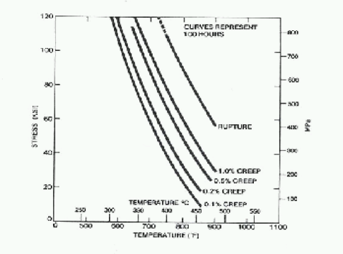
The immediate concern is to verify that eq. (1) could yield the desired order of magnitude for the small centrifugal stresses in our spacecraft, which is clearly determined by the exponential factor. Equating to s-1, we get eV at K, which seems quite reasonable. For example, the creep curves in Fig. 1 indicate and eV. Both and could vary considerably not only between materials, but even in a given sample, so the computation serves only to establish only the plausibility of this phenomenon as a cause of the anomaly. Moreover, the effective temperature for the spacecraft is probably significantly less than K, and its exponential contribution needs to be magnified by tidal action, as explained next.

Net expansion should result from the plastic flow in any case, because the centrifugal force is radial, and would cause the onboard material to stretch laterally as it is pulled outward. A lateral expanding stress is thus created by the cylindrical curvature of the centrifugal field, and the resulting dislocations would leave gaps in the lattice, forming microscopic breakages and causing creep. On earth, the spherical geometry of its gravitational pull produces a lateral compressive stress, forcing the dislocations to fill interstitial spaces and squeeze out atoms at the surface. The deformation rate due to these steady forces appears to be too low to account for the anomaly, as will be explained.
Considerable amplification is provided by tidal action, which not only periodically stretches the lattice, but rotates in the transverse plane, causing differential stretching between neighbouring regions of the lattice. As illustrated in Fig. 2, this significantly raises the probability of dislocation above that in a uniform stress, such as provided by the centrifugal and gravitational forces, where the neighbouring regions would be stretched or compressed to the same extent. For example, atom is subjected to stronger forces from and less from than it would ordinarily, so that it could be pushed or pulled out by , depending on the sign of the simultaneous lateral stress . The enhanced probability of dislocation means that the tidal action effectively lowers the dislocation “barrier” , by periodically injecting tidal energy into the lattice, so that the exponential factor in eq. (1) becomes . This is analogous to the action of the gate signal in a field-effect transistor (FET), which modulates the depletion region, and thence the net conductivity in the channel; the analogy is not perfect, however, because the dislocation density quickly reaches thermal equilibrium, returning the instantaneous plastic deformation rate to its steady stress value. However, the tidally induced dislocations would be of substantial density because of the periodicity of the lattice, and the incremental radial creep would make them irreversible upon withdrawal of the injected energy at each ebb. The resulting creep rate would therefore be proportional to the stress times the spin, which defines frequency of repetition of this tidal process.
Furthermore, in steady plastic flow, interactions between dislocations lead to the formation of lattice-like structures. The nonlinearity represented by in eq. (1) occurs because the dislocation lattices change dynamically with the stress and flow rate. In the tidally induced flow, the incremental creeps are purely transient, as described, and given the slowness of the phenomenon, the lattice conditions are not significantly altered between the successive tidal sweeps, so that the interactions between dislocations during these times are not much changed in the course of the flow. As a result, we would have identically for this component of the flow, yielding the formula
| (2) |
where and would both be different for the earth and for each spacecraft, and in the case of the spacecrafts including the dependence of the centrifugal force, and in the case of the earth.
Since we are only considering gross behaviour, we cannot depend on and alone to be responsible for matching the orders of magnitude between the two components of the anomaly, attributed to contraction on earth and expansion onboard, respectively. Variations in , due to varying distance from the sun and the aging of the RTG (radioactive thermoelectric generator), would cause the latter component to vary over each mission, as separately considered in §IV. For the moment, we still need to verify that the product is similar between the earth and the spacecraft, in order that the creep rates can be of similar magnitudes, viz - s-1. Taking Galileo as example, we find that its ton mass would produce a net centrifugal force of N at its spin axis, which is where the telemetry antenna and circuits are generally housed, about times smaller than the gravitational force on a comparable mass on earth. However, this particular spacecraft spins nominally at rpm, times faster than the earth, which leaves a factor of only to be made up by , , and possibly geometrical factors like .
I have thus shown that the repetitive action of a gravitational tidal force in the presence of a lateral stress produces cumulative expansion or contraction, depending on the sign of the stress, and further that the mechanism would be of the right magnitude for explaining both the Pioneer anomaly and the Hubble flow.
III Signal path analysis
I now establish, by analysing the actual process of measurement, how the Pioneer anomaly indisputably indicates the presence and involvement of both mechanisms, of expansion of the spacecraft and of contraction on earth. Moreover, the analysis will show that any complete explanation must introduce phenomena of identical behaviour, i.e. that a fundamentally different explanation is impossible.
The indication of the anomaly comprises an almost linearly increasing Doppler residual in the Pioneer’s ranging signal, which is equivalent to an unmodelled acceleration acting on the spacecraft in the same direction as the sun’s gravitational field Anderson1998 Turyshev1999 . That is, the data is not of the perceived acceleration itself, but of an increasing residual , so we must examine this first before turning to relativistic or mechanical causes for explaining actual acceleration. The reason such hypotheses by other researchers is that though the ranging procedure involves a different downlink frequency from the uplink, the possibility of drift, due to heat and circuit degradation, was assumed to have been completely eliminated by the use of a phase-locked loop (PLL) Bender1989 Vincent1990 Anderson1993 .
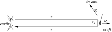
What has been overlooked is that the PLL cannot eliminate physical processes directly affecting the signal path, which would however impact the phase , where is the effective signal path and , the carrier wavelength, taken, for simplicity of argument, to be the constant over the entire round trip. The total path then comprises linear segments to and from the spacecraft, of length , plus an onboard segment representing the delay onboard the spacecraft, as illustrated in Fig. 3. The Doppler residual of Pioneer 10 Anderson1998 is thus indeed an acceleration
| (3) |
but the second derivative is of , not itself, as required for a kinematic acceleration. Instead, by using the signal path, we are no longer concerned with precise distribution of propagation delays and the refractive index, and can obtain the net impact on the path length more directly by integrating this phase acceleration, which yields
| (4) |
where the reported variations in the anomaly would be contained in . Eq. (4) has the exact form of Hubble’s law, as previously pointed out Prasad1999 , and the reported magnitude of the anomaly, s-1 Anderson1998 , makes approximately equal to the Hubble flow , whose accepted value km/s-Mpc is equal to s-1. The Pioneer anomaly is thus direct evidence of planetary Hubble flow, and there is no mathematical room for another explanation. I show further, in §V, that this conclusion is indeed consistent with the FRW model at this range, and that its existence was unobvious only because of current prejudices in relativistic cosmology.
The analysis invalidates Anderson et al.’s contention that a comparable effect is absent in planetary ranging data, as they considered only Mars and Venus, both less than AU from earth. As I have already shown Prasad2000c Prasad1999 , the ranging imprecision, which itself follows Hubble’s law in being proportional to , is at least 10 times too coarse for the detection of planetary Hubble flow indicated by the anomaly.
We can distinguish two separate contributions to , however, physical expansion of spacecraft material, causing the onboard path segment to increase, yielding , and expansion of the uplink and downlink spatial segments, each of length , the latter in effect describing expansion of space instead of matter. The latter notion would lead to contradiction when applied to our terrestrial unit referents of scale if interpreted according to the prevailing semantics of relativity (MTW, , p.719) (Rindler, , p.197), but it has a precise formal interpretation in terms of the relativity of scale Prasad2000c , and the likelihood of the requisite contraction at this rate has just been established in §II. We may accordingly break up as
| (5) |
where , to be attributed to contraction on earth, would be the constant component in all six missions. It would be recognised that would also contribute to the onboard segment, but this contribution can be conceptually absorbed in the spatial segments, leaving the onboard material expansion as the only contribution in ; in any case, as spatially, the net contribution from the would be negligibly small. Conversely implied is that the contribution must be disproportionately larger than the spatial extent of , which could be due to being much larger than for earth-bound materials, but this seems unlikely, as the ratio is rather large. On the other hand, substantial phase delay occurs over , and would be proportionally increased by physical expansion of the circuits, which has already been shown, in §II, to be not insubstantial.
IV Correlation of variations
While I have established planetary Hubble flow as the only possible explanation for the principal component , I have yet to show that material expansion onboard is the only one for . I do this now by deriving, from the notions of §II, the empirical model I had previously proposed to account for all variations of the anomaly Prasad1999 , which are particularly described by the best-fit curve given by Turyshev et al. Turyshev1999 , viz
| (6) |
where denoted the spacecraft’s spin, , the net gravitational force acting on the spacecraft, mostly due to the sun. The anisotropy factor means that the expansion, per each tidal sweep, cannot be assumed to be the same in all directions, as the spacecraft are not homogeneous blobs of matter. Given the nominal spin of rpm, the Hz peak fluctuation rate during Galileo’s earth fly-by Turyshev1999 , seems to be a clear symptom of physical features in the onboard signal path individually subtending ∘ at the axis, which seems quite reasonable judging from the diagrams available on NASA’s Galileo Web site.
It was subsequently pointed out to me that this inclusion of cannot be precise, as tidal action depends not on , but on its gradient , as implicitly considered in §II. Eq. (6) was, however, intended to be capable of accommodating any order of derivative whatsoever that might be uncovered by subsequent investigation; for example, since
| (7) |
a direct dependence on would have been represented by . However, as the magnitude of even at AU is only N/kg-m, tidal action by itself could not have been the driving force for the onboard expansion, but the centrifugal force, of the order of N, clearly could, for which . The angular dependence, denoted by the vector product, survives, however, as the tidal action “gates” the expansion, as described. We must also include the temperature dependence from eq. (2), which was unfortunately omitted in eq. (6), and absorb into , to arrive at the correct model for the effect of onboard tidal distension,
| (8) |
As described in Prasad1999 , the angular dependence, due to the fact that the spin axis generally points toward the earth and subtends an angle with the sun’s gravitational pull, would explain the almost linear falloff of the anomaly between and AU. and not the magnitude of is material, explains why the linearity holds in the - AU range regardless of the falloff of the sun’s pull and the falloff of its tidal action. At the other extreme, both at the perihelion and during earth-flybys, the spin axis would be normal to the sun at least at the instants of observation, in order to ensure the maximum angular separation from the sun for the ground telemetry antennas; this, together with the generally higher temperature due to proximity to the sun, seems adequate to account for very high values of the anomaly seen at these times.
The angular dependence had also prompted a conjecture that the residual difference between the Pioneers 10 and 11 could be at least partly due to the angles made with respect to the galactic centre. A more precise argument can now be made in retrospect, that though the sun’s gravitation even at AU is much stronger than the galactic field, m/s2 vs. m/s2, the solar contribution to the onboard expansion would be vastly diminished, as the spacecraft spin axes would be pointing almost directly toward the sun. Eq. (8) now provides a second factor that could be just as significant, viz the temperature , because Pioneer 11, which exhibits the larger residual anomaly, is both slightly younger, so that its RTG generates more heat than Pioneer 10’s, and is headed into the heliopause. However, differences in the construction of these craft, affecting and , as already explained, may turn out to be more influential than either of these hypotheses.
My contention that this is the only possible explanation of the variations in the anomaly, appears to be no weaker than the mathematical inference of planetary Hubble flow given above (eq. 4). The oscillatory characteristic of the NASA-JPL best-fit curve cannot be modelled without introducing a sinusoidal factor. Its apparent synchronisation with the earth’s orbit and asymmetries consistent with occlusion by the sun Prasad1999 , suffice to relate its phase to the earth’s relative position; as the linear falloff from to AU is then adequately modelled by the sine factor, we cannot have any other that would change substantially in this range. Since an oscillation ( Hz) substantially greater than the spin frequency (- rpm) was observed, we must include an anistropy factor . As we have no room left for or its derivatives, we need an amplification factor that particularly contributes at the perihelions, where both the tidal action and the temperature might be substantial, but at the other extreme, only would survive to contribute to the residual difference between the two Pioneers. The Boltzmann factor appears to be the simplest form for the inclusion of , and the scale factor then acquires natural interpretation as activation energy. We also find, from eqs. (4) and (5), that the result must represent an expansion of the signal path in some way, suggesting plastic flow, and discover not only that the Boltzmann form indeed occurs in the theory of dislocations and creep, but that the anomaly is consistent with the known values of creep under macroscopic stresses. Finally, the dependence on the subtended angle indicates an involvement of tidal action, but this cannot by itself provide net flow; a driving stress is required and is readily identified with the centrifugal and gravitational forces on the spacecraft and on earth, respectively. We still need a dependence on spin, not only in order to match the magnitudes of the and components, as explained in §II, but to also account for the changes in the anomaly coinciding with the changes in the spin frequency Turyshev1999 .
V Time-variant quantum scale
It should be clear that the mechanism of tidal contraction or expansion is a general principle that would hold for any particulate structure of matter in which the particles have well-defined mean locations, as there would be attractive and repulsive interactions between particles at these positions to which the reasoning of Fig. 2 could be applied. We would expect to find it operating in glasses, for example, and within Bose condensates not necessarily made of atoms, but not within liquids or gases, which has a geophysical significance to be described later. There is also disparity in the rates of contraction one would expect between materials, as the rates depend on and . The disparities are of interest as the particulate density would not be preserved in the interior of the lattice, and could become detectable via their impact on the electronic energy levels, for instance. But this appears unlikely, as the thermal interactions would be sufficient, given the slowness of the phenomenon, to even out the rate disparities and make the contraction uniform and continuous on earth. This is particularly true in the measurement of spectra, which by definition require the observations to last long enough for the instrument state to settle.
A more important consequence is the appearance of a Hubble flow in an otherwise steady universe to the terrestrial, shrinking observer Prasad2000c , which can now be fully appreciated in terms of the quantum picture, as follows. Recall that in every quantum measurement, the outcome is determined by an amplitude of the form , where if denote the variable being measured, must represent the data value that would be returned whenever the variable would be subsequently left in the state , which, of course, is quantified by the probability . As a result, must represent a macroscopic physical state of the observing system, and this makes every distance-related measurement susceptible to the effects of the contraction, as itself becomes time-variant, causing the amplitudes to vanish except for s which are time-varying the same way.

Fig. 4 shows a wave being received by a detector, and the latter’s ongoing shrinkage, indicated by the arrow. Since a photon absorption must correspond to the smallest possible change between the stationary states of the detector, which means a whole “antinodal lobe”, i.e. the portion of a standing wave between adjacent nodes, the detector can only detect waves that fill an exact number of antinodal lobes in the detector, as depicted for the lower order wave in the figure. The properties that make these antinodal lobes specially significant are:
-
i.
Their energies are dependent only on their electromagnetic amplitudes, and not a priori on the frequency or wavelength, which makes them the right classical candidates, in place of whole modes, for thermal equipartition.
- ii.
-
iii.
An equilibrial equipartition over such lobes does yield Planck’s law for the cavity spectrum Prasad2000a , and these two principles of stationarity and antinodal equipartition have been further shown to be sufficient for deducing the correct form of quantisation in the interactions of matter Prasad2000b .
Properties (ii) and (iii) are the reason that every photon detector behaves as a resonant cavity; property (i) of course provides the crucial conceptual link to classical mechanics that has been missing in the 20th-century physics, which enables us to consider the physics of shrinking observers beyond simplistic philosophical terms (cf. (MTW, , p719)), and to deduce a redshift conforming to Hubble’s law, as follows.
To obtain the form of the stationary states of a shrinking detector, we take the stationary waves , for the nonshrinking detector, and insert an increasing scale factor to compensate for the shrinkage along the linear dimension. This yields , which is Parker’s solution for the wave equation in the FRW metric Parker1988
| (9) |
which we in turn interpret, in our context, as describing the apparent scaling of all space in the perspective of the shrinking observer, to whom the detector eigenstate must appear to be a uniform wave. In reality, as would be seen by nonshrinking observers, the wavelength of this eigenstate must correspondingly decrease with distance as shown. The shrinking detector can thus strike a momentary resonance, as required for photon detection by (ii), at wavelength at range and at at range , both differing from the wavelength at the detector. This apparent redshift, seen by the shrinking observer, may be thought of as a virtual Doppler effect, as the apparent expansion of space, eq. (9), implies a virtual recession of all objects. However, to explain the effect from the perspective of the nonshrinking observers, we cannot simply count the wavefronts crossing the detector boundary () as in prior theory, because that would fail to take the contraction into account and thus include waves which cannot be detected.
We are therefore forced to count only the waves which would measure a fixed number of antinodal lobes within the detector, which would be of if they had started out at and if they had begun at , because the detector would have shrunk by and over their respective times of flight and . Additionally, since we clearly have no logical room for issues of dispersion, as in Parker’s theory, must be strictly linear,
| (10) |
and , literally following Hubble’s law. This is readily interpreted as saying that only the instantaneous value of , the contraction rate, can possibly affect our immediate observation.
More particularly, eq. (10) yields the acceleration formula , which, as stated at the outset, exactly matches the observed Prasad2000c . The linearity clearly holds at any scale of measurement in our theory, unlike the current thinking in relativistic cosmology, where both and are commonly assumed to operate only on intergalactic scale. In fact, the equations of the relativistic theory (cf. (Wald, , p98)) do not involve any variable or relation to formally incorporate this prejudice, and it is therefore not surprising that they do predict an incremental acceleration Cooperstock1998
| (11) |
where is the orbital frequency ( s-1) and , the present epoch ( s). This at first seems to be too small to correlate with the Pioneer anomaly, but the involvement of obfuscates the scalability of eq. (11). Instead, from our preceding formula for acceleration, which in effect includes , we directly obtain
| (12) |
closely matching the anomalous time dilation rate s-1 Anderson1998 , and supporting all earlier conjectures of the cosmological connection of the anomaly Rosales1998 Ellman1998 Prasad1999 .
More importantly, it means that the conceptual foundations of relativistic cosmology, based on Mach’s philosophy Einstein1911 , are not only imprecise, in not taking the observer’s referents as the basis of relativity Prasad2000c , but also at variance with the empirical evidence of both , for which the standard model ideas lead to speculations of large scale repulsion, and of the Pioneer anomaly, for which modifications to gravitational field theory were being considered (cf. Anderson1998 ). It also invalidates the big bang and related notions of the standard model, though it may yet be possible to reinterpret some of its results in light of the present discovery of tidal contraction, as I did for the Doppler theory of the Hubble redshift. The in eq. (12) cannot, of course, be interpreted as the present age of the universe in the present theory, and is recognisable as in disguise, obtained from the large scale measurements.
Conclusion
It should be mentioned that any ongoing contraction could reproduce the Hubble flow, including descent within a gravitational well; but the descent would have to be at over km/s in order to explain the Hubble flow Prasad2000c . The Pioneer anomaly is the first direct evidence of planetary Hubble flow resulting from a contraction of referents, but as just shown, our prejudicial views prevented us both from recognising this and from predicting it in prior theory. This is just as well, because we might then have lacked the motivation to explain the variational part (§IV), and the tidal mechanisms would have been much harder to uncover. Instead, as even this connection was not obvious at the outset, precise logical foundations of both relativity and quantum mechanics have been discovered in the course of this investigation, while the key mechanism itself has been demonstrated to be of macroscopic origin and to scale correctly with routine measurements of creep.
While the problem of the Pioneer anomaly has been completely solved thus essentially by creep, the significance of the result is hard to overestimate. As formally predicted and now shown, it invalidates all our current notions of cosmology, as the Hubble redshift, on which they were fundamentally based, has been shown to be the result of a strictly terrestrial mechanism. It is worth noting that the arguments of §V are not dependent on the acceptability of the logical foundations mentioned above, as the only property of antinodal lobes critically used, (ii), follows immediately from Planck’s law . The uniformity of contraction was independently argued to result from a basic rule of spectral measurement, that sufficient time be allowed beyond that required for thermal stability of the detector’s state, which is consistent with Landauer’s principle relating thermalisation and data states Landauer1961 . While the contraction itself is consistent with ordinary creep data in terms of magnitude, the driving mechanism for the compaction, or distension aboard the deep space probes, appears to be sound and adequately scales between the earth and the spinning spacecraft. I have also previously shown that considerable evidence of past expansion of the earth Runcorn1965 Wesson1973 , which remain unresolved Wesson1999pvt , as well as the measured lunar recession Lunar1994 , are consistent with the Hubble flow on these scales MacDougall1963 Prasad1999 , and this, as shown in §V, would be consistent with the relativistic theory, but not with the prior views. Against this, I make no attempt to reinterpret or dismiss the existing results of the big bang theory, such as the cosmic microwave background (CMB), Olbers’ paradox or inflation, as these issues appear to be secondary to that of correctness and acceptability of the terrestrial contraction.
The explanation of the past expansion evidence is interesting in its own right, as we no longer have to deal with an overall expansion of the earth. This would have required difficult hypotheses of ongoing creation of matter, which fell short on the required magnitude by a full order Wesson1973 NarliKem1988 . The evidence is principally that the continents must have not only once formed one contiguous mass, but also that this mass should have once completely covered the earth Runcorn1965 . The present theory resolves this difficulty perfectly, as the contraction would have caused the sialic masses to break apart, forming the tectonic plates, and to continuously widen the gaps between the continents, independently of the tectonic motions, as the contraction does not apply to liquid or gaseous matter. The total widening should be about mm/y, corresponding to an apparent expansion of the earth’s radius, as seen by earth-bound observers to whom the continents would not appear to be shrinking, by about mm/y Creer1965 ; this may be verifiable by GPS measurements now or in the near future.
It was also of concern to me that attributing a third of the lunar recession to the Hubble flow Prasad2000c Prasad1999 might lead to inconsistency with the known cause of tidal friction, which is necessary to explain the slowing down of the earth’s spin. This problem too is now resolved, as we can now recognise, from §II, that the Hubble component itself requires the earth’s spin to do work in shrinking the sialic matter.
We would also expect find this mechanism operating on every planetary body with a solid surface and subject to tidal action. We do find such markings on Europa, which is subject to strong tidal forces from Jupiter and Ganymede, and on Mars, which does suffer tidal action from the sun, but the contribution remains to be estimated in either of these cases. Correspondingly, we expect to find an expansion occurring in every spinning spacecraft, but none in the others; since spin seems to be necessary for achieving the stability needed for the measurement Anderson1998 , the antennae and electronics subsystems used for the ranging would have to be despun for verifying this conclusion.
Acknowledgements.
Special thanks are owed to Bruce G Elmegreen and a referee for posing the key issues that led to this answer, and to ASM International for their kind permission to reproduce the creep curves in Fig. 1.References
- (1) V Guruprasad. Relativity of spatial scale and of the Hubble flow: The logical foundations of relativity and cosmology. gr-qc/0005014, May 2000.
- (2) A G Reiss et al. Observational evidence from supernovae for an accelerating universe and a cosmological constant. Astro J, 1998.
- (3) P M Garnavich et al. Constraints on cosmological models… Ap J Lett, 493:53, 1998.
- (4) B Leibundgut et al. The high-redshift supernova search – evidence for a positive cosmological constant. Dark’98, 1998. astro-ph/9812042.
- (5) P M Garnavich et al. Supernova limits on the cosmic equation of state. Ap J, 509 issue 1:74–79, 1998.
- (6) J D Anderson et al. Indication from Pioneer 10/11, Galileo and Ulysses data of an apparent anomalous, weak, long-range acceleration. Phys Rev Lett, Oct 1998.
- (7) S G Turyshev et al. The apparent anomalous … XXXIV Rencontres de Moriond, France, Jan 1999, Mar 1999. gr-qc/9903024.
- (8) S K Runcorn. Earth, possible expansion of. In Intl Dict of Geophysics, pages 383–389. Pergamon, 1967.
- (9) P S Wesson. The implications for geophysics of modern cosmologies in which is variable. Quarterly J of Roy Astro Soc, pages 9–64, 1973.
- (10) P S Wesson. Private communication, 1999.
- (11) V Guruprasad. Stationarity + wall jitter = Planck: The correct thermodynamics of radiation. physics/0003041, Apr 2000.
- (12) V Guruprasad. Entanglement, thermalisation and stationarity: The computational foundations of quantum mechanics. quant-ph/0005021, May 2000.
- (13) V Guruprasad. The correct analysis and explanation of the Pioneer-Galileo anomalies. astro-ph/9907363, 1999.
- (14) Ti-6Al-4V Alloy: Solution Treated and Aged Bar. In H E Boyer, editor, Atlas of Creep and Stress-Rupture Curves, page 22.11. ASM International, Materials Park, OH 44073-002, 1988.
- (15) McGraw-Hill Encyclopaedia of Science & Technology. McGraw-Hill, 1997.
- (16) P L Bender and M A Vincent. Small Mercury Relativity Orbiter. Technical Report N90-19940 12-90, NASA, Aug 1989.
- (17) M A Vincent and P L Bender. Orbit determination and gravitational field accuracy for a Mercury transponder satellite. J Geophy Res, 95:21357–21361, Dec 1990.
- (18) J D Anderson et al. Gravitational wave background in coincidence experiments with Doppler tracking of interplanetary spacecraft. Am Astro Soc Meeting, 182(05.11), May 1993.
- (19) C W Misner, K S Thorne, and J A Wheeler. Gravitation. W H Freeman and Co, 1973.
- (20) W Rindler. Essential Relativity. Springer-Verlag, 2nd edition, 1977.
- (21) L Parker. Particle creation by expansion of the universe. In V M Canuto and B G Elmegreen, editors, Handbook of Astronomy, Astrophysics and Geophysics, volume II. Gordon and Breach, 1988.
- (22) R M Wald. General Relativity. Univ of Chicago, 1984.
- (23) F I Cooperstock, V Faraoni, and D N Vollick. The influence of cosmological expansion on local systems. astro-ph/9803097, 1998.
- (24) J L Rosales and J L Sanchez-Gomez. A possible cosmological origin of the indicated anomalous acceleration … gr-qc/9810085, Oct 1998.
- (25) R Ellman. An interpretation of the Pioneer 10/11 … Phys Rev Lett, 81(14):5, Oct 1998.
- (26) A Einstein. On the influence of gravitation on the propagation of light (1911). In The principle of relativity. Dover, 1952.
- (27) R Landauer. Irreversibility and Heat Generation in the Computing Process. IBM Journal, Jul 1961.
- (28) J O Dickey et al. Lunar laser ranging: A continuing legacy of the Apollo program. Science, 265, jul 1994.
- (29) J MacDougall et al. A comparison of terrestrial and universal expansion. Nature, 199:1080, 1963.
- (30) J V Narlikar and A K Kembhavi. Non-standard Cosmologies. In V M Canuto and B G Elmegreen, editors, Handbook of Astronomy, Astrophysics and Geophysics, volume II. Gordon and Breach, 1988.
- (31) K M Creer. An expanding earth? Nature, 205:539, 1965.