Efficient and Extensible Algorithms for Multi Query Optimization

Abstract

Complex queries are becoming commonplace, with the growing use of decision support systems. These complex queries often have a lot of common sub-expressions, either within a single query, or across multiple such queries run as a batch. Multi-query optimization aims at exploiting common sub-expressions to reduce evaluation cost. Multi-query optimization has hither-to been viewed as impractical, since earlier algorithms were exhaustive, and explore a doubly exponential search space.

In this paper we demonstrate that multi-query optimization using heuristics is practical, and provides significant benefits. We propose three cost-based heuristic algorithms: Volcano-SH and Volcano-RU, which are based on simple modifications to the Volcano search strategy, and a greedy heuristic. Our greedy heuristic incorporates novel optimizations that improve efficiency greatly. Our algorithms are designed to be easily added to existing optimizers. We present a performance study comparing the algorithms, using workloads consisting of queries from the TPC-D benchmark. The study shows that our algorithms provide significant benefits over traditional optimization, at a very acceptable overhead in optimization time.

1 Introduction

Complex queries are becoming commonplace, especially due to the advent of automatic tools that help analyze information from large data warehouses. These complex queries often have a lot of common sub-expressions since i) they make extensive use of views which are referred to multiple times in the query and ii) many of them are correlated nested queries in which parts of the inner subquery may not depend on the outer query variables, thus forming a common sub-expression for repeated invocations of the inner query.

The scope for finding common sub-expressions increases greatly if we consider a set of queries executed as a batch. For example, SQL-3 stored procedures may invoke several queries, which can be executed as a batch. Data analysis/reporting often requires a batch of queries to be executed. The work of [SHT⁺99] on using relational databases for storing XML data, has found that queries on XML data, written in a language such as XML-QL [XML98], need to be translated into a sequence of relational queries.

The task of updating a set of related materialized views also generates related queries with common sub-expressions [RSS96]. Materialized views are increasingly being supported by commercial database systems, and are used to speed up query processing. In particular, data warehouses, which store large volumes of data, depend on materialized aggregate views for efficient query processing, and the materialized views as well as expressions to incrementally update them tend to have significant amounts of common subexpressions. Sharing of common subexpressions is also of importance when the expressions access remote data, and are therefore expensive [SV98, FLMS99].

In this paper, we address the problem of optimizing sets of queries which may have common sub-expressions; this problem is referred to as multi-query optimization. We note here that common subexpressions are possible even within a single query; the techniques we develop deal with such intra-query common subexpressions as well.

Traditional query optimizers are not appropriate for optimizing queries with common sub expressions, since they make locally optimal choices, and may miss globally optimal plans as the following example demonstrates.

Example 1.1

Let $Q_{1}$ and $Q_{2}$ be two queries whose locally optimal plans (i.e., individual best plans) are $(R\Join S)\Join P$ and $(R\Join T)\Join S$ respectively. The best plans for $Q_{1}$ and $Q_{2}$ do not have any common sub-expressions. However, if we choose the alternative plan $(R\Join S)\Join T$ (which may not be locally optimal) for $Q_{2}$, then, it is clear that $R\Join S$ is a common sub-expression and can be computed once and used in both queries. This alternative with sharing of $R\Join S$ may be the globally optimal choice.

On the other hand, blindly using a common sub-expression may not always lead to a globally optimal strategy. For example, there may be cases where the cost of joining the expression $R\Join S$ with $T$ is very large compared to the cost of the plan $(R\Join T)\Join S$; in such cases it may make no sense to reuse $R\Join S$ even if it were available. $\Box$

Example 1.1 illustrates that the job of multi-query optimization, over and above that of ordinary query optimization, is to (i) recognize the possibilities of shared computation, and (ii) modify the optimizer search strategy to explicitly account for shared computation and find a globally optimal plan.

While there has been work on multi-query optimization in the past ([Sel88b, SSN94, SG90, CLS93, PS88]), prior work has concentrated primarily on exhaustive algorithms. Other work has concentrated on finding common subexpressions as a post-phase to query optimization [Fin82, SV98], but this gives limited scope for cost improvement. (We discuss related work in detail in Section 7.) The search space for multi-query optimization is doubly exponential in the size of the queries, and exhaustive strategies are therefore impractical; as a result, multi-query optimization was hitherto considered too expensive to be useful.

In this paper we show how to make multi-query optimization practical, by developing novel heuristic algorithms, and presenting a performance study that demonstrates their practical benefits.

Our algorithms are based on an AND-OR DAG representation [Rou82, RR82, GM91] to compactly represents alternative query plans. The DAG representation ensures that they are extensible, in that they can easily handle new operations and transformation rules. The DAG can be constructed as in [GM91, PGLK97], with some extensions to ensure that all common sub-expressions are detected and unified. The DAG construction also takes into account sharing of computation based on “subsumption” – examples of such sharing include computing $\sigma_{A<5}(E)$ from the result of $\sigma_{A<10}(E)$.

The task of the heuristic optimization algorithms is then to decide what subexpressions should be materialized and shared. Two of the heuristics we present, Volcano-SH and Volcano-RU are lightweight modifications of the Volcano optimization algorithm. The third heuristic is a greedy strategy which iteratively picks the subexpression that gives the maximum benefit (reduction in cost) if it is materialized and reused. One of our important contributions here lies in three novel optimizations of the greedy algorithm implementation, that make it very efficient. These are as follows:

1. We present a novel incremental algorithm for computing benefits of materializing different subexpressions.

   The motivation for incrementality is as follows. The greedy strategy performs a large number of benefit computations, with different sets of subexpressions chosen to be materialized. Specifically, having picked a set $X$ of subexpressions to materialize, to find the next one to materialize, the greedy strategy must compute the benefit of every other subexpression $x$ that is a candidate.

   Having processed the earlier mentioned AND-OR DAG for finding benefit of materializing subexpression $x_{1}$ (having already materialized a set of subexpressions $X$), our incremental algorithm is able to compute the benefit of materializing a different subexpression $x_{2}$ incrementally, without revisiting the whole of the DAG.

2. The benefit of materializing a subexpression depends on what else is materialized. Suppose we computed the benefit of materializing subexpressions $x_{1},x_{2},\ldots,x_{n}$, and expression $x_{k}$ was chosen by greedy. The next round of greedy has to recompute benefits of all the remaining $x_{i}$’s, which can be expensive.

   We present a monotonicity based technique for greatly reducing the number of benefit recomputations required.

3. We present an algorithm for computing sharability of subexpressions, allowing the greedy algorithm to be applied only to sharable nodes.

Our performance studies show that each of these optimizations leads to a great improvement in the performance of the greedy algorithm.

In addition to choosing what intermediate expression results to materialize and reuse, our optimization framework also chooses physical properties, such as sort order, for the materialized results. Our algorithms also handle the choice of what (temporary) indices to create on materialized results/database relations.

Our algorithms can be easily extended to perform multi-query optimization on nested queries as well as multiple invocations of parameterized queries (with different parameter values). We also note that our algorithms can be made to work with System R style bottom-up optimizers.

We have implemented a query optimizer based on the Volcano optimization framework, and modified it to implement all our multi-query optimization algorithms, at an additional effort of around 3500 lines of code.

We conducted a performance study of our multi-query optimization algorithms, using queries from the TPC-D benchmark as well as other queries based on the TPC-D schema. Our study demonstrates not only savings based on estimated cost, but also significant improvements in actual run times on a commercial database.

Our performance results show that our multi-query optimization algorithms give significant benefits over single query optimization, at an acceptable extra optimization time cost. The extra optimization time is more than compensated by the execution time savings. All three heuristics beat the basic Volcano algorithm, but in general greedy produced the best plans, followed by Volcano-RU and Volcano-SH.

We believe that in addition to our technical contributions, another of our contributions lies in showing how to engineer a practical multi-query optimization system — one which can smoothly integrate extensions, such as indexes and nested queries, allowing them to work together seamlessly. In summer ’99, our algorithms were partially prototyped on the Microsoft SQL Server optimizer, and multi-query optimization is currently being evaluated by Microsoft for possible inclusion in SQL Server.

The rest of the paper is structured as follows: We describe how to set up the search space for multi-query optimization in Section 2. The Volcano-SH and the Volcano-RU heuristics are described in Section 3. The greedy algorithm is described in Section 4. Our extensions to create indexes on intermediate relations and nested queries are discussed in Sections 5. We describe the results of our performance study in Section 6. Section 7 discusses related work, while Section 8 discusses directions for future work. We present our conclusions in Section 9.

2 Setting Up The Search Space For Multi-Query Optimization

As we mentioned in Section  1, the job of a multi-query optimizer is to (i) recognize possibilities of shared computation (thus essentially setting up the search space by identifying common sub-expressions) and (ii) modify the optimizer search strategy to explicitly account for shared computation and find a globally optimal plan. Both of the above tasks are important and crucial for a multi-query optimizer but are orthogonal. In other words, the details of the search strategy do not depend on how aggressively we identify common sub-expressions (of course, the efficacy of the strategy does). We have explored both the above tasks in detail, but choose to emphasize the search strategy component of our work in this paper, for lack of space. However, we outline the high level ideas and the intuition behind our algorithms for identifying common sub-expresions in this section and refer to the full version of the paper [RSSB98] for details at the appropriate locations in this section.

Before we describe our algorithms for identifying common-sub expressions, we describe the AND-OR DAG representation of queries. An AND–OR DAG is a directed acyclic graph whose nodes can be divided into AND-nodes and OR-nodes; the AND-nodes have only OR-nodes as children and OR-nodes have only AND-nodes as children.

An AND-node in the AND-OR DAG corresponds to an algebraic operation, such as the join operation ($\Join$) or a select operation ($\sigma$). It represents the expression defined by the operation and its inputs. Hereafter, we refer to the AND-nodes as operation nodes. An OR-node in the AND-OR DAG represents a set of logical expressions that generate the same result set; the set of such expressions is defined by the children AND nodes of the OR node, and their inputs. We shall refer to the OR-nodes as equivalence nodes henceforth.

Figure 1: Initial Query and DAG Representations

The given query tree is initially represented directly in the AND-OR DAG formulation. For example, the query tree of Figure 1(a) is initially represented in the AND-OR DAG formulation, as shown in Figure 1(b). Equivalence nodes (OR-nodes) are shown as boxes, while operation nodes (AND-nodes) are shown as circles.

The initial AND-OR DAG is then expanded by applying all possible transformations on every node of the initial query DAG representing the given set of queries. Suppose the only transformations possible are join associativity and commutativity. Then the plans $A\Join(B\Join C)$ and $(A\Join C)\Join B$, as well as several plans equivalent to these modulo commutativity can be obtained by transformations on the initial AND-OR-DAG of Figure 1(b). These are represented in the DAG shown in Figure 1(c). We shall refer to the DAG after all transformations have been applied as the expanded DAG. Note that the expanded DAG has exactly one equivalence node for every subset of $\{A,B,C\}$; the node represents all ways of computing the joins of the relations in that subset.

We use the techniques of [GM91] to efficiently generate the AND-OR DAG representing the query. We also use the optimizations of [PGLK97], which avoid duplicate derivations due to join associativity/commutativity. As shown in [PGLK97], the time complexity of top-down DAG generation for the case of joins is then the same as for bottom-up join-order enumeration as in System R style optimizers. For lack of space we omit details of DAG generation; details may be found in [RSSB98].

2.1 Extensions to DAG Generation For Multi-Query Optimization

To apply multi-query optimization to a batch of queries, the queries are represented together in a single DAG, sharing subexpressions. To make the DAG rooted, a pseudo operation node is created, which does nothing, but has the root equivalence nodes of all the queries as its inputs.

We now outline two extensions to the DAG generation algorithm to aid multi-query optimization.

The first extension deals with identification of common subexpressions. If a query contains two subexpressions that are logically equivalent, but syntactically different, (e.g., $(A\Join B)\Join C$, and $A\Join(B\Join C)$) the initial query DAG would contain two different equivalence nodes representing the two subexpressions. We modify the Volcano DAG generation algorithm so that whenever it finds nodes to be equivalent (after applying join associativity) it unifies the nodes, replacing them by a single equivalence node.

The Volcano algorithm uses a hashing scheme to detect repeated derivations, and avoids creating duplicate equivalence nodes due to cyclic derivations (e.g., expression $e1$ is transformed to $e2$, which is then transformed back to $e1$). Our modification additionally uses the hashing scheme to detect and unify duplicate equivalence nodes that were either pre-existing or got created by transformations from different expressions. Details of unification may be found in [RSSB98].

The second extension is to detect and handle subsumption. For example, suppose two subexpressions $e1$: $\sigma_{A<5}(E)$ and $e2$: $\sigma_{A<10}(E)$ appear in the query. The result of $e1$ can be obtained from the result of $e2$ by an additional selection, i.e., $\sigma_{A<5}(E)\equiv\sigma_{A<5}(\sigma_{A<10}(E))$. To represent this possibility we add an extra operation node $\sigma_{A<5}$ in the DAG, between $e1$ and $e2$. Similarly, given $e3$: $\sigma_{A=5}(E)$ and $e4$: $\sigma_{A=10}(E)$, we can introduce a new equivalence node $e5$: $\sigma_{A=5\vee A=10}(E)$ and add new derivations of $e3$ and $e4$ from $e5$. The new node represents the sharing of accesses between the two selection. In general, given a number of selections on an expression $E$, we create a single new node representing the disjunction of all the selection conditions. Similar derivations also help with aggregations. For example, if we have $e6$: ${}_{dno}{\cal G}_{sum(Sal)}(E)$ and $e7$: ${}_{age}{\cal G}_{sum(Sal)}(E)$, we can introduce a new equivalence node $e8$: ${}_{dno,age}{\cal G}_{sum(Sal)}(E)$ and add derivations of $e6$ and $e7$ from equivalence node $e8$ by further groupbys on $dno$ and $age$.

The idea of applying an operation (such as $\sigma_{A<5}$ on one subexpression to generate another has been proposed earlier [Rou82, Sel88b, SV98]. Integrating such options into the AND-OR DAG, as we do, clearly separates the space of alternative plans (represented by the DAG) from the optimization algorithms. Thereby, it simplifies our optimization algorithms, allowing them to avoid dealing explicitly with such derivations.

2.2 Physical AND-OR DAG

Properties of the results of an expression, such as sort order, that do not form part of the logical data model are called physical properties [GM91]. Physical properties of intermediate results are important, since e.g. if an intermediate result is sorted on a join attribute, the join cost can potentially be reduced by using a merge join. This also holds true of intermediate results that are materialized and shared.

It is straightforward to refine the above AND-OR DAG representation to represent physical properties and obtain a physical AND-OR DAG. Our search algorithms can be easily understood on the above AND-OR DAG representation (without physical properties), although they actually work on physical DAGs. Therefore, for brevity, we do not explicitly consider physical properties further; for details see [RSSB98]. Our implementation indeed handles physical properties.

3 Reuse Based Multi-Query Optimization Algorithms

In this section we study a class of multi-query optimization algorithms based on reusing results computed for other parts of the query. We present these as extensions of the Volcano optimization algorithm. Before we describe the extensions, in Section 3.1, we very briefly outline the basic Volcano optimization algorithm, and how to extend it to find best plans given some nodes in the DAG are materialized. Sections 3.2 and 3.3 then present two of our heuristic algorithms, Volcano-SH and Volcano-RU.

3.1 Volcano Optimization Algorithm and Materialized Views

The Volcano optimization algorithm operates on the expanded DAG generated earlier. It finds the best plan for each node by performing a depth first traversal of the DAG starting from that node as follows. Costs are defined for operation and equivalence nodes. The cost of an operation node $o$ is defined as follows:
          $cost(o)=$ cost of executing $(o)$ + $\Sigma_{e_{i}\in children(o)}cost(e_{i})$
The children of $o$ (if any) are equivalence nodes. The cost of an equivalence node $e$ is given as
          $cost(e)=min\{cost(o_{i})|o_{i}\in children(e)\}$
and is $0$ if the node has no children (i.e., it represents a relation).

Volcano also caches the best plan it finds for each equivalence node, in case the node is re-visited during the depth first search of the DAG. A branch and bound pruning is also performed by carrying around a cost limit; for simplicity, we disregard pruning in this paper. For lack of space we omit details, but refer readers to [GM91].

Now we consider how to extend Volcano to find best plans, given that (expressions corresponding to) some equivalence nodes in the DAG are materialized. Let $reusecost(m)$ denote the cost of reusing the materialized result of $m$, and let $M$ denote the set of materialized nodes.

To find the cost of a node given a set of nodes $M$ have been materialized, we simply use the Volcano cost formulae above, with the following change. When computing the cost of a operation node $o$, if an input equivalence node $e$ is materialized (i.e., in $M$), use the minimum of $reusecost(e)$ and $cost(e)$ when computing $cost(o)$. Thus, we use the following expression instead:
          $cost(o)=$ cost of executing $(o)$ + $\Sigma_{e_{i}\in children(o)}C(e_{i})$
                 where $C(e_{i})=cost(e_{i})$ if $e_{i}\not\in M$, and $=min(cost(e_{i}),reusecost(e_{i}))$ if $e_{i}\in M$.

3.2 The Volcano-SH Algorithm

In our first strategy, which we call Volcano-SH, the expanded DAG is first optimized using the basic Volcano optimization algorithm. The best plan computed for the virtual root is the combination of the Volcano best plans for each individual query. The best plans produced by the Volcano optimization algorithm may have common subexpressions. Thus the consolidated best plan for the root of the DAG may contain nodes with more than one parent, and is thus a DAG-structured plan. The Volcano-SH algorithm works on the above consolidated best plan, and decides in a cost based manner which of the nodes to materialize and share.

Since materialization of a node involves storing the result to the disk, and we assume pipelined execution of operators, it may be possible for recomputation of a node to be cheaper than the cost of materializing and reusing the node. In fact, in our experiments in Section 6, there were quite a few occasions when it was cheaper to recompute an expression.

Let us consider first a naive (and incomplete) solution. Consider an equivalence node $e$. Let $cost(e)$ denote the computation cost of node $e$. Let $numuses(e)$ denote the number of times node $e$ is used in course of execution of the plan. Let $matcost(e)$ denote the cost of materializing node $e$. As before, $reusecost(e)$ denote the cost of reusing the materialized result of $e$. Then, we decide to materialize $e$ if

$$cost(e)+matcost(e)+reusecost(e)\times(numuses(e)-1)<numuses(e)\times cost(e)$$

The left hand side of this inequality gives the cost of materializing the result when first computed, and using the materialized result thereafter; the right hand side gives the cost of the alternative wherein the result is not materialized but recomputed on every use. The above test can be simplified to

$$matcost(e)/(numuses(e)-1)+reusecost(e)<cost(e)$$ (1)

The problem with the above solution is that $numuses(e)$ and $cost(e)$ both depend on what other nodes have been materialized, For instance, suppose node $e_{1}$ is used twice in computing node $e_{2}$, and node $e_{2}$ is used twice in computing node $e_{3}$. Now, if no node is materialized, $e_{1}$ is used four times in computing $e_{3}$. If $e_{2}$ is materialized, $e_{1}$ gets used twice in computing $e_{2}$, and $e_{2}$ gets computed only once. Thus, materializing $e_{2}$ can reduce both $numuses(e_{1})$ and $cost(e_{3})$.

In general, $numuses(e)$ depends on which ancestors of $e$ in the Volcano best plan are materialized, and $cost(e)$ depends on which descendants have been materialized. Specifically, $numuses(e)$ can be computed recursively based on the number of uses of the parents of $e$: $numuses(root)=1$, while for all other nodes, $numuses(e)=\sum_{p\in parents(e)}U(p)$, where $U(p)=numuses(p)$ if $p$ is not materialized, and $=1$ if $p$ is materialized. Thus, computing $numuses$ requires us to know the materialization status of parents. On the other hand, as we have seen earlier, $cost(e)$ depends on what descendants have been materialized.

A naive exhaustive strategy to decide what nodes in the Volcano best plan to materialize is to consider each subset of the nodes in the best plan, and compute the cost of the best plan given that all nodes in this subset are materialized at their first computation; the subset giving the minimum cost is selected for actual materialization. Unfortunately, this strategy is exponential in the number of nodes in the Volcano best plan, and therefore is very expensive; we require cheaper heuristics.

Procedure Volcano-SH($P$)
Input:		Consolidated Volcano best plan $P$ for virtual root of DAG
Output:		Set of nodes to materialize $M$, and the corresponding best plan $P$
Global variable: $M$, the set of nodes chosen to be materialized
	$M=\{~{}\}$
	Perform prepass on $P$ to introduce subsumption derivations
	Let $C_{root}=$ ComputeMatSet($root$)
	Set $C_{root}=C_{root}+\sum_{d\in M}(cost(d)+matcost(d))$
	Undo all subsumption derivations on $P$ where the subsumption node is not chosen to be materialized.
	return (M,P)
Procedure ComputeMatSet$(e)$
	If $cost(e)$ is already memoized, return $cost(e)$
	Let operator $o_{e}$ be the child of $e$ in $P$
	For each input equivalence node $e_{i}$ of $o_{e}$
		Let $C_{i}$= ComputeMatSet($e_{i}$)      // returns computation cost of $e_{i}$
		If $e_{i}$ is materialized, let $C_{i}=reusecost(e_{i})$
	Compute $cost(e)$ = cost of operation $o_{e}$ + $\sum_{i}C_{i}$
	If ($matcost(e)/(numuses^{-}(e)-1)+reusecost(e)<cost(e)$)
		If $e$ is not introduced by a subsumption derivation
			add $e$ to $M$       // Decide to materialize $e$
		else if $cost(e)+matcost(e)+reusecost(e)*(numuses^{-}(e)-1)$ is less than
				savings to parents of $e$ due to introducing materialized $e$
			add $e$ to $M$       // Decide to materialize $e$
	Memoize and return $cost(e)$

Figure 2: The Volcano-SH Algorithm

To avoid enumerating all sets as above, the Volcano-SH algorithm, which is shown in Figure 2, traverses the tree bottom-up. As each equivalence node $e$ is encountered in the traversal, Volcano-SH decides whether or not to materialize $e$. When making a materialization decision for a node, the materialization decisions for all descendants ia already known. When Volcano-SH is examining a node $e$, let $M$ denote the set of descendants of $e$ that have been chosen to be materialized. Based on this, we can compute $cost(e)$ for a node $e$, as described in Section 3.1.

To make a materialization decision for a node $e$, we also need to know $numuses(e)$. Unfortunately, $numuses(e)$ depends on the materialization status of its parents, which is not fixed yet. To solve this problem, the Volcano-SH algorithm uses an underestimate $numuses^{-}(e)$ of number of uses of $e$. Such an underestimate can be obtained by simply counting the number of ancestors of $e$ in the Volcano best plan. We use this underestimate in our cost formulae, to make a conservative decision on materialization.

Based on the above, Volcano-SH makes the decision on materialization as follows: node $e$ is materialized if

$$matcost(e)/(numuses^{-}(e)-1)+reusecost(e)<cost(e)$$ (2)

Note that here we use the lower bound $numuses^{-}(e)$ in place of $numuses(e)$. Using the lower bound guarantees that if we decide to materialize a node, materialization will result in cost savings.

The final step of Volcano-SH is to factor in the cost of computing and materializing all nodes that were chosen to be materialized. Thus, to the cost of the pseudoroot computed as above, we add $\sum_{m\in M}(cost(m)+matcost(m))$, where $M$ is the set of nodes chosen to be materialized.

Let us now return to the first step of Volcano-SH. Note that the basic Volcano optimization algorithm will not exploit subsumption derivations, such as deriving $\sigma_{A<5}(E)$ by using $\sigma_{A<5}(\sigma_{A<10}(E))$, since the cost of the latter will be more than the former, and thus will not be locally optimal.

To consider such plans, we perform a pre-pass, checking for subsumption amongst nodes in the plan produced by the basic Volcano optimization algorithm. If a subsumption derivation is applicable, we replace the original derivation by the subsumption derivation. At the end of Volcano-SH, if the shared subexpression is not chosen to be materialized, we replace the derivation by the original expressions. In the above example, in the prepass we replace $\sigma_{A<5}(E)$ by $\sigma_{A<5}(\sigma_{A<10}(E))$. If $\sigma_{A<10}(E)$ is not materialized, we replace $\sigma_{A<5}(\sigma_{A<10}(E))$ by $\sigma_{A<5}(E)$.

The algorithm of [SV98] also finds best plans and then chooses which shared subexpressions to materialize. Unlike Volcano-SH, it does not factor earlier materialization choices into the cost of computation.

3.3 The Volcano-RU Algorithm

The intuition behind Volcano-RU is as follows. Consider $Q_{1}$ and $Q_{2}$ from Example 1.1. With the best plans as shown in the example, namely $(R\Join S)\Join P$ and $(R\Join T)\Join S$, no sharing is possible with Volcano-SH. However, when optimizing $Q_{2}$, if we realize that $R\Join S$ is already used in in the best plan for $Q_{1}$ and can be shared, the choice of plan $(R\Join S)\Join T$ may be found to be the best for $Q_{2}$.

The intuition behind the Volcano-RU algorithm is therefore as follows. Given a batch of queries, Volcano-RU optimizes them in sequence, keeping track of what plans have already been chosen for earlier queries, and considering the possibility of reusing parts of the plans. The resultant plan depends on the ordering chosen for the queries; we return to this issue after discussing the Volcano-RU algorithm.

Procedure Volcano-RU
Input:		Expanded DAG on queries $Q_{1},\ldots,Q_{k}$ (including subsumption derivations)
Output:		Set of nodes to materialize $M$, and the corresponding best plan $P$
	$N$ = $\phi$ // Set of potentially materialized nodes
	For each equivalence node $e$, Set $count[e]=0$
	For $i=1$ to $k$
		Compute $P_{i}$, the best plan for $Q_{i}$, using Volcano, assuming nodes in $N$ are materialized
		For every equivalence node in $P_{i}$
			set $count[e]=count[e]+1$
			If ($cost(e)+matcost(e)+count[e]*reusecost(e)<(count[e]+1)*cost(e)$)
					// Worth materializing if used once more
				add $e$ to set $N$
	Combine $P_{1},\ldots,P_{k}$ to get a single DAG-structured plan $P$
	(M,P) = Volcano-SH($P$)       // Volcano-SH makes final materialization decision

Figure 3: The Volcano-RU Algorithm

The pseudocode for the Volcano-RU algorithm is shown in Figure 3. Let $Q_{1},\ldots,Q_{n}$ be the queries to be optimized together (and thus under the same pseudo-root of the DAG). The Volcano-RU algorithm optimizes them in the sequence $Q_{1},\ldots,Q_{n}$. After optimizing $Q_{i}$, we note equivalence nodes in the DAG that are part of the best plan $P_{i}$ for $Q_{i}$ as candidates for potential reuse later. We maintain counts of number of uses of these nodes. We also check if each node is worth materializing, if it is used one more time. If so, we add the node to $N$, and when optimizing the next query, we will assume it to be available materialized.

Thus, in our example earlier in this section, after finding the best plan for the first query, we check if $R\Join S$ is worth materializing if it is used once more. If so we add it to $N$, and assume it to be materialized when optimizing the second query.

After optimizing all the individual queries, the second phase of Volcano-RU executes Volcano-SH on the overall best plan found as above to further detect and exploit common subexpressions. This step is essential since the earlier phase of Volcano-RU does not consider the possibility of sharing common subexpressions within a single query – equivalence nodes are added to $N$ only after optimizing an entire query. Adding a node to $N$ in our algorithm does not imply it will get reused and therefore materialized. Instead Volcano-SH makes the final decision on what nodes to materialize. The difference from directly applying Volcano-SH to the result of Volcano optimization is that the plan $P$ that is given to Volcano-SH has been chosen taking sharing of parts of earlier queries into account, unlike the Volcano plan.

A related implementation issue is in caching of best plans in the DAG. When optimizing $Q_{i}$ we cache best plans in nodes of the DAG that are descendants of $Q_{i}$. When optimizing a later query $Q_{j}$, if we find a node that is not in $P_{i}$ (the plan chosen for query $Q_{i}$) for some $i<j$, we must recompute the best plan for the node; for, the set of nodes $M$ may have changed, leading to a different best plan. Therefore we note with each cached best plan which query was being optimized when the plan was computed; we recompute the plan as required above.

Note that the result of Volcano-RU depends on the order in which queries are considered. In our implementation we consider the queries in the order in which they are given, as well as in the reverse of that order, and pick the cheaper one of the two resultant plans. Note that the DAG is still constructed only once, so the extra cost of considering the two orders is relatively quite small. Considering further (possibly random) orderings is possible, but the optimization time would increase further.

4 The Greedy Algorithm

In this section, we present the greedy algorithm, which provides an alternative approach to the algorithms of the previous section. Our major contribution here lies in how to efficiently implement the greedy algorithm, and we shall concentrate on this aspect.

In this section, we present an algorithm with a different optimization philosophy. The algorithm picks a set of nodes $S$ to be materialized and then finds the optimal plan given that nodes in $S$ are materialized. This is then repeated on different sets of nodes $S$ to find the best (or a good) set of nodes to be materialized.

Before coming to the greedy algorithm, we present some definitions, and an exhaustive algorithm. As before, we shall assume there is a virtual root node for the DAG; this node has as input a “no-op” logical operator whose inputs are the queries $Q_{1}\ldots Q_{k}$. Let $Q$ denote this virtual root node.

For a set of nodes $S$, let $bestcost(Q,S)$ denote the cost of the optimal plan for $Q$ given that nodes in $S$ are to be materialized (this cost includes the cost of computing and materializing nodes in $S$). As described in the Volcano-SH algorithm, the basic Volcano optimization algorithm with an appropriate definition of the cost for nodes in $S$ can be used to find $bestcost(Q,S)$.

To motivate our greedy heuristic, we first describe a simple exhaustive algorithm. The exhaustive algorithm, iterates over each subset $S$ of the set of nodes in the DAG, and chooses the subset $S_{opt}$ with the minimum value for $bestcost(Q,S)$. Therefore, $bestcost(Q,S_{opt})$ is the cost of the globally optimal plan for $Q$.

It is easy to see that the exhaustive algorithm is doubly exponential in the size of the initial query DAG and is therefore impractical.

In Figure 4 we outline a greedy heuristic that attempts to approximate $S_{opt}$ by constructing it one node at a time. The algorithm iteratively picks nodes to materialize. At each iteration, the node $x$ that gives the maximum reduction in the cost if it is materialized is chosen to be added to $X$.

Procedure Greedy
Input:		Expanded DAG for the consolidated input query $Q$
Output:		Set of nodes to materialize and the corresponding best plan
	X = $\phi$
	Y = set of equivalence nodes in the DAG
	while (Y $\neq\phi$)
L1:		Pick the node x $\in$ Y with the smallest value for bestcost(Q, {x} $\cup$ X)
		if (bestcost(Q, {x} $\cup$ X) $<$ bestcost(Q, X) )
			Y = Y - x;   X = X $\cup$ {x}
		else Y = $\phi$ // benefit $<$ 0, so break out of loop
	return X

Figure 4: The Greedy Algorithm

The greedy algorithm as described above can be very expensive due to the large number of nodes in the set $Y$ and the large number of times the function $bestcost$ is called. We now present three important and novel optimizations to the greedy algorithm which make it efficient and practical.

1. The first optimization is based on the observation that the nodes materialized in the globally optimal plan are obviously a subset of the ones that are shared in some plan for the query. Therefore, it is sufficient to initialize $Y$ in Figure 4, with nodes that are shared in some plan for the query. We call such nodes sharable nodes. For instance, in the expanded DAG for $Q_{1}$ and $Q_{2}$ corresponding to Example 1.1, $R\Join S$ is sharable while $R\Join T$ is not. We present an efficient algorithm for finding sharable nodes in Section 4.1.

2. The second optimization is based on the observation that there are many calls to $bestcost$ at line L1 of Figure 4, with different parameters. A simple option is to process each call to $bestcost$ independent of other calls. However, observe that the symmetric difference in the sets passed as parameters to successive calls to $bestcost$ is very small – sucessive calls take parameters of the form $bestcost(Q,\{x\}\cup X)$, where only $x$ varies. It makes sense for a call to leverage the work done by a previous call. We describe a novel incremental cost update algorithm, in Section 4.2, that maintains the state of the optimization across calls to $bestcost$, and incrementally computes a new state from the old state.

3. The third optimization, which we call the monotonicity heuristic, avoids having to invoke $bestcost(Q,$ $\{x\}\cup X)$, for every $x\in Y$, in line L1 of Figure 4. We describe this optimization in detail in Section 4.3.

4.1 Sharability

In this subsection, we outline how to detect whether an equivalence node can be shared in some plan. The plan tree of a plan is the tree obtained from the DAG structured plan, by replicating all shared nodes of the plan, to completely eliminate sharing. The degree of sharing of a logical equivalence node in an evaluation plan $P$ is the number of times it occurs in the plan tree of $P$. The degree of sharing of a logical equivalence node in an expanded DAG is the maximum of the degree of sharing of the equivalence node amongst all evaluation plans represented by the DAG. A logical equivalence node is sharable if its degree of sharing in the expanded DAG is greater than one.

We now present a simple algorithm to compute the degree of sharing of each node and thereby detect whether a node is shared. A sub–DAG of a node $x$ consists of the nodes below $x$ along with the edges between these nodes that are in the original DAG. For each node $x$ of the DAG, and every node $z$ in the sub-DAG rooted at $x$, let $E[x][z]$ represent the degree of sharing of $z$ in the sub–DAG rooted at $x$. Clearly for all nodes $x$, $E[x][x]$ is $1$. For a given node $x$, all other $E[x][\_]$ values can be computed given the values $E[y][\_]$ for all children $y$ of $x$ as follows.

If $x$ is an operation node
         $E[x][z]=Sum\{E[y][z]~{}|~{}y\in children(x)\}$
and if $x$ is an equivalence node,
         $E[x][z]=Max\{E[y][z]~{}|~{}y\in children(x)\}$
The degree of sharing of a node $z$ in the overall DAG is given by $E[r][z]$, where $r$ is the root of the DAG.

Space is minimized in the above by computing $E[x][z]$ for one $z$ at a time, discarding all but $E[r][z]$ at the end of computation for one $z$ value.

A reasonable implementation of the above algorithm has time complexity proportional to the number of non-zero entries in $E$, which in the worst case is proportional to the square of the number of nodes in the DAG. However, typically, $E$ is fairly sparse since the DAG is typically “short and fat” – as the number of queries grows, the height of the DAG may not increase, but it becomes wider. Thus, as expected, this sharability computation algorithm is fairly efficient in practice. In fact, for the queries we considered in our performance study (Section 6), the computation took at most a few tens of milliseconds.

4.2 Incremental Cost Update

The sets with which $bestcost$ is called successively at line L1 of Figure 4 are closely related, with their (symmetric) difference being very small. For, line L1 finds the node $x$ with the maximum benefit, which is implemented by calling $bestcost(Q,\{x\}\cup X)$, for different values of $x$. Thus the second parameter to $bestcost$ changes by dropping one node $x_{i}$ and adding another $x_{i+1}$. We now present an incremental cost update algorithm that exploits the results of earlier cost computations to incrementally compute the new plan.

Function UpdateCost($S$, $S^{\prime}$)
// PropHeap is a priority heap (initially empty), containing // equivalence nodes ordered by their topological sort number add $S-S^{\prime}\cup S^{\prime}-S$ to PropHeap
while (PropHeap is not empty)
	$N$ = equivalence node with minimum topological sort number in PropHeap
	Remove $N$ from PropHeap
	oldCost = old value of cost($N$)
	cost($N$) = Min $\{$ cost($p$) — $p\in children(N)\}$ // $children(N)$ are operation nodes
	if (cost($N$) $\neq$ oldCost) or $N\in(S-S^{\prime})$ or $N\in(S^{\prime}-S)$
		for every parent operation node $p$ of $N$
			cost($p$) = cost of executing operation $p$ + $\sum_{c\in children(p)}(C(c))$
				where $C(c)$ = cost($c$) if $c\not\in S^{\prime}$, and $=min(reusecost(c),$ cost($c$)) if $c\in S^{\prime}$
			add $p$’s parent equivalence node to PropHeap if not already present
TotalCost = $compcost(root)+\sum_{s\in S^{\prime}}($cost($s$) $+matcost(s))$

Figure 5: Incremental Cost Update

Figure 5 outlines our incremental cost update algorithm. Let $S$ be the set of nodes shared at a given point of time, i.e., the previous call to $bestcost$ was with $S$ as the parameter. The incremental cost update algorithm maintains the cost of computing every equivalence node, given that all nodes in $S$ are shared, and no other node is shared. Let $S^{\prime}$ be the new set of nodes that are shared, i.e., the next call to $bestcost$ has $S^{\prime}$ as the parameter. The incremental cost update algorithm starts from the nodes that have changed in going from $S$ to $S^{\prime}$ (i.e., nodes in $S^{\prime}-S$ and $S-S^{\prime}$) and propagates the change in cost for the nodes upwards to all their parents; these in turn propagate any changes in cost to their parents if their cost changed, and so on, until there is no change in cost. Finally, to get the total cost we add the cost of computing and materializing all the nodes in $S^{\prime}$.

If we perform this propagation in an arbitrary order then in the worst case we could propagate the change in cost through a node $x$ multiple times (for example, once from a node $y$ which is an ancestor of another node $z$ and then from $z$). A simple mechanism for avoiding repeated propagation uses topological numbers for nodes of the DAG. During DAG generation the DAG is sorted topologically such that a descendant always comes before an ancestor in the sort order, and nodes are numbered in this order. As shown in Figure 5, cost propagation is performed in the topological number ordering using PropHeap, a heap built on the topological number. The heap is used to efficiently find the node with the minimum topological sort number at each step.

In our implementation, we additionally take care of physical property subsumption. Details of how to perform incremental cost update on physical DAGs with physical property subsumption are given in [RSSB98].

4.3 The Monotonicity Heuristic

In Figure 4, the function $bestcost$ will be called once for each node in $Y$, under normal circumstances. We now outline how to determine the node with the smallest value of $bestcost$ much more efficiently, using the monotonicity heuristic.

Let us define $benefit(x,X)$ as $bestcost(Q,X)-bestcost(Q,\{x\}\cup X)$. Notice that, minimizing $bestcost$ in line $L1$ corresponds to maximizing benefit as defined here. Suppose the benefit is monotonic. Intuitively, the benefit of a node is monotonic if it never increases as more nodes get materialized; more formally $benefit$ is monotonic if $\forall X\supseteq Y$, $benefit(x,X)\leq benefit(x,Y)$.

We associate an upper bound on the benefit of a node in $Y$ and maintain a heap ${\cal C}$ of nodes ordered on these upper bounds. The initial upper bound on the benefit of a node in $Y$ uses the notion of the maximum degree of sharing of the node (which we described earlier). The initial upper bound is then just the cost of evaluating the node (without any materializations) times the maximum degree of sharing. The heap ${\cal C}$ is now used to efficiently find the node $x\in Y$ with the maximum $benefit(x,X)$ as follows: Iteratively, the node $n$ at the top ${\cal C}$ is chosen, its current benefit is recomputed, and the heap ${\cal C}$ is reordered. If $n$ remains at the top, it is deleted from the ${\cal C}$ heap and chosen to be materialized and added to $X$. Assuming the monotonicity property holds, the other values in the heap are upper bounds, and therefore, the node $n$ added to $X$ above, is indeed the node with the maximum real benefit.

If the monotonicity property does not hold, the node with maximum current benefit may not be at the top of the heap ${\cal C}$ , but we still use the above procedure as a heuristic for finding the node with the greatest benefit. Our experiments in Section 6 demonstrate that the above procedure greatly speeds up the greedy algorithm. Further, for all queries we experimented with, the results were exactly the same even if the monotonicity heuristic was not used.

5 Extensions

In this section, we briefly outline extensions to i) incorporate creation and use of temporary indices, ii) optimize nested queries to exploit common sub-expressions and iii) optimize multiple invocations of parameterized queries.

Costs may be substantially reduced by creating (temporary) indices on database relations or materialized intermediate results. To incorporate index selection, we model the presence of an index as a physical property, similar to sort order. Since our algorithms are actually executed on the physical DAG, they choose not only what results to materialize but also what physical properties they should have. Index selection then falls out as simply a special case of choosing physical properties, with absolutely no changes to our algorithms.

Next we consider nested queries. One approach to handling nested queries is to use decorrelation techniques (see, e.g. [SPL96]). The use of such decorrelation techniques results in the query being transformed to a set of queries, with temporary relations being created. Now, the queries generated by decorrelation have several subexpressions in common, and are therefore excellent candidates for multi-query optimization. One of the queries in our performance evaluation brings out this point.

Correlated evaluation is used in other cases, either because it may be more efficient on the query, or because it may not be possible to get an efficient decorrelated query using standard relational operations [RR98]. In correlated evaluation, the nested query is repeatedly invoked with different values for correlation variables. Consider the following query.

Query: select * from a, b, c
       where a.x = b.x and b.y = c.y and
             a.cost = (select min(a1.cost) from  a as a1, b as b1
                       where a1.x = b1.x and b1.y = c.y)

One option for optimizing correlated evaluation of this query is to materialize $a\Join b$, and share it with the outer level query and across nested query invocations. An index on $a\Join b$, on attribute $b.y$ is required for efficient access to it in the nested query, since there is a selection on $b.y$ from the correlation variable. If the best plan for the outer level query uses the join order $(a\Join b)\Join c$, materializing and sharing $a\Join b$ may provide the best plan.

In general, parts of the nested query that do not depend on the value of correlation variables can potentially be shared across invocations [RR98]. We can extend our algorithms to consider such reuse across multiple invocations of a nested query. The key intuition is that when a nested query is invoked many times, benefits due to materialization must be multiplied by the number of times it is invoked; results that depend on correlation variables, however, must not be considered for materialization. The nested query invariant optimization techniques of [RR98] then fall out as a special case of ours.

Our algorithms can also be extended to optimize multiple invocations of parameterized queries. Parameterized queries are queries that take parameter values, which are used in selection predicates; stored procedures are a common example. Parts of the query may be invariant, just as in nested queries, and these can be exploited by multi-query optimization.

These extensions have been implemented in our system; details may be found in [RSSB98].

6 Performance Study

Our algorithms were implemented by extending and modifying a Volcano-based query optimizer we had developed earlier. All coding was done in C++, with the basic optimizer taking approx. 17,000 lines, common MQO code took 1000 lines, Volcano-SH and Volcano-RU took around 500 lines each, and Greedy took about 1,500 lines.

The optimizer rule set consisted of select push down, join commutativity and associativity (to generate bushy join trees), and select and aggregate subsumption. Our implementation incorporates the optimizations of [PGLK97] which, for join transformations, prevent repeated derivations of the same expressions.

Implementation algorithms included sort-based aggregation, merge join, nested loops join, indexed join, indexed select and relation scan. Our implementation incorporates all the techniques discussed in this paper, including handling physical properties (sort order and presence of indices) on base and intermediate relations, unification and subsumption during DAG generation, and the sharability algorithm for the greedy heuristic.

The block size was taken as 4KB and our cost functions assume 6MB is available to each operator during execution (we also conducted experiments with larger memory sizes up to 128 MB, with similar results). Standard techniques were used for estimating costs, using statistics about relations. The cost estimates contain an I/O component and a CPU component, with seek time as 10 msec, transfer time of 2 msec/block for read and 4 msec/block for write, and CPU cost of 0.2 msec/block of data processed. We assume that intermediate results are pipelined to the next input, using an iterator model as in Volcano; they are saved to disk only if the result is to be materialized for sharing. The materialization cost is the cost of writing out the result sequentially.

The tests were performed on a single processor 233 Mhz Pentium-II machine with 64 MB memory, running Linux. Optimization times are measured as CPU time (user+system).

6.1 Basic Experiments

The goal of the basic experiments was to quantify the benefits and cost of the three heuristics for multi-query optimization, Volcano-SH, Volcano-RU and Greedy, with plain Volcano-style optimization as the base case. We used the version of Volcano-RU which considers the forward and reverse orderings of queries to find sharing possibilities, and chooses the minimum cost plan amongst the two.

Experiment 1 (Stand-Alone TPCD):

The workload for the first experiment consisted of four queries based on the TPCD benchmark. We used the TPCD database at scale of 1 (i.e., 1 GB total size), with a clustered index on the primary keys for all the base relations. The results are discussed below and plotted in Figure 6.

  

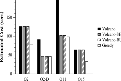
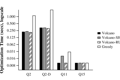
Figure 6: Optimization of Stand-alone TPCD Queries

TPCD query Q2 has a large nested query, and repeated invocations of the nested query in a correlated evaluation could benefit from reusing some of the intermediate results. For this query, though Volcano-SH and Volcano-RU do not lead to any improvement over the plan of estimated cost 126 secs. returned by Volcano, Greedy results in a plan of with significantly reduced cost estimate of 79 secs. Decorrelation is an alternative to correlated evaluation, and Q2-D is a (manually) decorrelated version of Q2 (due to decorrelation, Q2-D is actually a batch of queries). Multi-query optimization also gives substantial gains on the decorrelated query Q2-D, resulting in a plan with estimated costs of 46 secs., since decorrelation results in common subexpressions. Clearly the best plan here is multi-query optimization coupled with decorrelation.

Observe also that the cost of Q2 (without decorrelation) with Greedy is much less than with Volcano, and is less than even the cost of Q2-D with plain Volcano — this results indicates that multi-query optimization can be very useful in other queries where decorrelation is not possible. To test this, we ran our optimizer on a variant of Q2 where the in clause is changed to not in clause, which prevents decorrelation from being introduced without introducing new internal operators such as anti-semijoin [RR98]. We also replaced the correlated predicate $PS\_PARTKEY=P\_PARTKEY$ by $PS\_PARTKEY\not=P\_PARTKEY$. For this modified query, Volcano gave a plan with estimated cost of 62927 secs., while Greedy was able to arrive at a plan with estimated cost 7331, an improvement by almost a factor of 9.

We next considered the TPCD queries Q11 and Q15, both of which have common subexpressions, and hence make a case for multi-query optimization. For Q11, each of our three algorithms lead to a plan of approximately half the cost as that returned by Volcano. Greedy arrives at similar improvements for Q15 also, but Volcano-SH and Volcano-RU do not lead to any appreciable benefit for this query.

Overall, Volcano-SH and Volcano-RU take the same time and space as Volcano. Greedy takes more time than the others for all the queries, but the maximum time taken by greedy over the four queries was just under 2 seconds, versus 0.33 seconds taken by Volcano for the same query. The extra overhead of greedy is negligible compared to its benefits. The total space required by Greedy ranged from 1.5 to 2.5 times that of the other algorithms, and again the absolute values were quite small (up to just over 130KB).

Results on Microsoft SQL-Server 6.5:

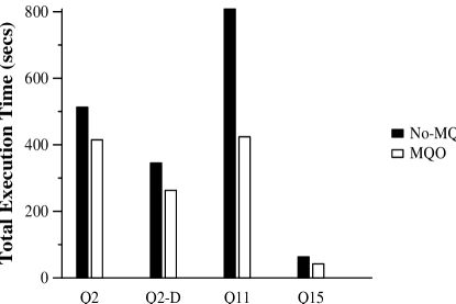
Figure 7: Execution of Stand-alone TPCD Queries on MS SQL Server

To study the benefits of multi-query optimization on a real database, we tested its effect on the queries mentioned above, executed on Microsoft SQL Server 6.5, running on Windows NT, on a 333 Mhz Pentium-II machine with 64MB memory. We used the TPCD database at scale 1 for the tests. To do so, we encoded the plans generated by Greedy into SQL. We modeled sharing decisions by creating temporary relations, populating, using and deleting them. If so indicated by Greedy, we created indexes on these temporary relations. We could not encode the exact evaluation plan in SQL since SQL-Server does its own optimization. We measured the total elapsed time for executing all these steps.

The results are shown in Figure 7. For query Q2, the time taken reduced from 513 secs. to 415 secs. Here, SQL-Server performed decorrelation on the original Q2 as well as on the result of multi-query optimization. Thus, the numbers do not match our cost estimates, but clearly multi-query optimization was useful here. The reduction for the decorrelated version Q2-D was from 345 secs. to 262 secs; thus the best plan for Q2 overall, even on SQL-Server, was using multi-query optimization as per Greedy on a decorrelated query. The query Q11 speeded up by just under 50%, from 808 secs. to 424 secs.  and Q15 from 63 secs. to 42 secs. using plans with sharing generated by Greedy.

The results indicate that multi-query optimization gives significant time improvements on a real system. It is important to note that the measured benefits are underestimates of potential benefits, for the following reasons. (a) Due to encoding of sharing in SQL, temporary relations had to be stored and re-read even for the first use. If sharing were incorporated within the evaluation engine, the first (non-index) use can be pipelined, reducing the cost further. (b) The operator set for SQL-Server 6.5 seems to be rather restricted, and does not seem to support sort-merge join; for all queries we submitted, it only used (index)nested-loops. Our optimizer at times indicated that it was worthwhile to materialize the relation in a sorted order so that it could be cheaply used by a merge-join or aggregation over it, which we could not encode in SQL/SQL-Server.

In other words, if multi-query optimization were properly integrated into the system, the benefits are likely to be significantly larger, and more consistent with benefits according to our cost estimates.

Experiment 2 (Batched TPCD Queries):

In the second experiment, the workload models a system where several TPCD queries are executed as a batch. The workload consists of subsequences of the queries Q3, Q5, Q7, Q9 and Q10 from TPCD; none of these queries has any common subexpressions within itself. Each query was repeated twice with different selection constants. Composite query BQi consists of the first i of the above queries, and we used composite queries BQ1 to BQ5 in our experiments. Like in Experiment 1, we used the TPCD database at scale of 1 and assumed that there are clustered indices on the primary keys of the database relations.

Note that although a query is repeated with two different values for a selection constant, we found that the selection operation generally lands up at the bottom of the best Volcano plan tree, and the two best plan trees may not have common subexpressions.

  

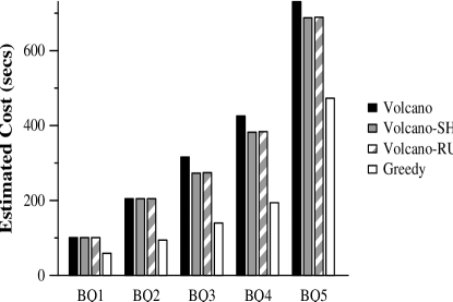
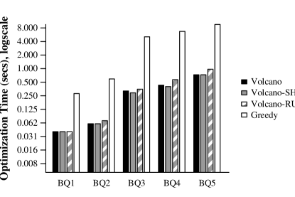
Figure 8: Optimization of Batched TPCD Queries

The results on the above workload are shown in Figure 8. Across the workload, Volcano-SH and Volcano-RU achieve up to only about 14% improvement over Volcano with respect to the cost of the returned plan, while incurring negligible overheads. There was no difference between Volcano-SH and Volcano-RU on these queries, implying the choice of plans for earlier queries did not change the local best plans for later queries. Greedy performs better, achieving up to 56% improvement over Volcano, and is uniformly better than the other two algorithms.

As expected, Volcano-SH and Volcano-RU have essentially the same execution time and space requirements as Volcano. Greedy takes about 10 seconds on the largest query in the set, BQ5, while Volcano takes about 0.7 second on the same. However, the estimated cost savings on BQ5 is 260 seconds, which is clearly much more than the extra optimization time cost of 10 secs. Thus the extra time spent on Greedy is well spent. Similarly, the space requirements for Greedy were more by about a factor of three to four over Volcano, but the absolute difference for BQ5 was only 60KB. The benefits of Greedy, therefore, clearly outweigh the cost.

6.2 Scaleup Analysis

To see how well our algorithms scale up with increasing numbers of queries, we defined a new set of 22 relations $PSP_{1}$ to $PSP_{22}$ with an identical schema $(P$, $SP$, $NUM)$ denoting part id, subpart id and number. Over these relations, we defined a sequence of 18 component queries $SQ_{1}$ to $SQ_{18}$: component query $SQ_{i}$ was a pair of chain queries on five consecutive relations $PSP_{i}$ to $PSP_{i+4}$, with the join condition being $PSP_{j}.SP=PSP_{j+1}.P$, for $j=i..i+3$. One of the queries in the pair $SQ_{i}$ had a selection $PSP_{i}.NUM\geq a_{i}$ while the other had a selection $PSP_{i}.NUM\geq b_{i}$ where $a_{i}$ and $b_{i}$ are arbitrary values with $a_{i}\not=b_{i}$.

To measure scaleup, we use the composite queries $CQ_{1}$ to $CQ_{5}$, where $CQ_{i}$ is consists of queries $SQ_{1}$ to $SQ_{4i-2}$. Thus, $CQ_{i}$ uses $4i+2$ relations $PSP_{1}$ to $PSP_{4i+2}$, and has $32i-16$ join predicates and $8i-4$ selection predicates. Query CQ5, in particular, is on 22 relations and has 144 join predicates and 36 select predicates. The size of the 22 base relations $PSP_{1},\ldots,PSP_{22}$ varied from 20000 to 40000 tuples (assigned randomly) with 25 tuples per block. No index was assumed on the base relations.

  

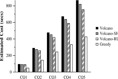
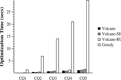
Figure 9: Optimization of Scaleup Queries

The cost of the plan and optimization time for the above workload is shown in Figure 9. The relative benefits of the algorithms remains similar to that in the earlier workloads, except that Volcano-RU now gives somewhat better plans than Volcano-SH. Greedy continues to be the best, although it is relatively more expensive. The optimization time for Volcano, Volcano-SH and Volcano-RU increases linearly. The increase in optimization time for Greedy is also practically linear, although it has a very small super-linear component. But even for the largest query, CQ5 (with 22 relations, 144 join predicates and 36 select predicates) the time taken was only 30 seconds. The size of the DAG increases linearly for this sequence of queries. From the above, we can conclude that Greedy is scalable to quite large query batch sizes.

To better understand the complexity of the Greedy heuristic on the scaleup workload, in addition to the optimization time we measured the total number of times cost propagation occurs across equivalence nodes, and the total number of times cost recomputation is initiated. The result is plotted in Figure 10. Note that in addition to the size of the DAG, the number of sharable nodes also increases linearly across queries CQ1 to CQ5.

  

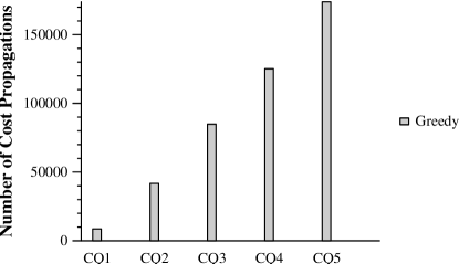
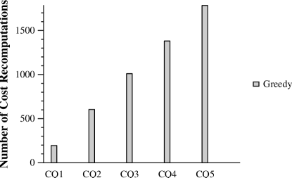
Figure 10: Complexity of the Greedy Heuristic

Greedy was considered expensive by [SDN98] because of its worst case complexity: it can be as much as $O(k^{2}e)$, where $k$ is the number of nodes in the DAG which are sharable, and $e$ is the number of edges in the DAG. However, for multi-query optimization, the DAG tends to be wide rather than tall – as we add queries, the DAG gets wider, but its height does not increase, since the height is defined by individual queries.

The result shows that for the given workload, the number of times cost propagation occurs across equivalence nodes, and the number of times cost recomputation is initiated both increase almost linearly with number of queries. The observed complexity is thus much less than the worst case complexity.

The number of times costs are propagated across equivalence nodes is almost constant per cost recomputation. This is because the number of nodes of the DAG affected by a single materialization does not vary much with number of queries, which is exploited by incremental cost recomputation. The height of the DAG remains constant (since the number of relations per query is fixed, which is a reasonable assumption).

6.3 Effect of Optimizations

In this series of experiments, we focus on the effect of individual optimizations on the optimization of the scaleup queries. We first consider the effect of the monotonicity heuristic addition to Greedy. Without the monotonicity heuristic, before a node is materialized the benefits would be recomputed for all the sharable nodes not yet materialized. With the monotonicity heuristic addition, we found that on an average only about 45 benefits were recomputed each time, across the range of CQ1 to CQ5. In contrast, without the monotonicity heuristic, even at CQ2 there were about 1558 benefit recomputations each time, leading to an optimization time of 77 seconds for the query, as against 7 seconds with monotonicity. Scaleup is also much worse without monotonicity. Best of all, the plans produced with and without the monotonicity heuristic assumption had virtually the same cost on the queries we ran. Thus, the monotonicity heuristic provides very large time benefits, without affecting the quality of the plans generated.

To find the benefit of the sharability computation, we measured the cost of Greedy with the sharability computation turned off; every node is assumed to be potentially sharable. Across the range of scaleup queries, we found that the optimization time increased significantly. For CQ2, the optimization time increased from 30 secs. to 46 secs. Thus, sharability computation is also a very useful optimization.

In summary, our optimizations of the implementation of the greedy heuristic result in an order of magnitude improvement in its performance, and are critical for it to be of practical use.

6.4 Discussion

To check the effect of memory size on our results, we ran all the above experiments increasing the memory available to the operators from 6MB to 32MB and further to 128MB. We found that the cost estimates for the plans decreased slightly, but the relative gains (i.e., cost ratio with respect to Volcano) essentially remained the same throughout for the different heuristics.

We stress that while the cost of optimization is independent of the database size, the execution cost of a query, and hence the benefit due to optimization, depends upon the size of the underlying data. Correspondingly, the benefit to cost ratio for our algorithms increase markedly with the size of the data. To illustrate this fact, we ran the batched TPCD query BQ5 (considered in Experiment 2) on TPCD database with scale of 100 (total size 100GB). Volcano returned a plan with estimated cost of 106897 seconds while Greedy obtains a plan with cost estimate 73143 seconds, an improvement of 33754 seconds. The extra time spent during optimization is 10 seconds, as before, which is negligible relative to the gain.

While the benefits of using MQO show up on query workloads with common subexpressions, a relevant issue is the performance on workloads with rare or nonexistent overlaps. If it is known apriori that the workload is not going to benefit from MQO, then we can set a flag in our optimizer that bypasses the MQO related algorithms described in this paper, reducing to plain Volcano.

To study the overheads of our algorithms in a case with no sharing, we took TPCD queries Q3, Q5, Q7, Q9 and Q10, renamed the relations to remove all overlaps between queries, and created a batch consisting of the queries with relations renamed. The overheads of Volcano-SH and Volcano-RU are neglibible, as discussed earlier. Basic Volcano optimization took 650 msec, while the Greedy algorithm took 820 msec. Thus the overhead was around 25%, but note that the absolute numbers are very small. With no overlap, the sharability detection algorithm finds no node sharable, causing the Greedy algorithm to terminate immediately (returning the same plan as Volcano). Thus, the overhead in Greedy is due to (a) expansion of the entire DAG, and (b) the execution of the sharability detection algorithm. Of this overhead, cause (a) is predominant, and the sharability computation was quite cheap on queries with no sharing.

In our experiments, Volcano-RU was better than Volcano-SH only in a few cases, but since their run times are similar, Volcano-RU is preferable. There exist cases where Volcano-RU finds out plans as good as Greedy in a much less time and using much less space; but on the other hand, in the above experiments we saw many cases where additional investment of time and space in Greedy pays off and we get substantial improvements in the plan.

To summarize, for very low cost queries, which take only a few seconds, one may want to use Volcano-RU, which does a “quick-and-dirty” job; especially so if the query is also syntactically complex. For more expensive queries, as well as “canned” queries that are optimized rarely but executed frequently over large databases, it clearly makes sense to use Greedy.

7 Related Work

The multi-query optimization problem has been addressed in [Fin82, Sel88b, SSN94, SG90, CLS93, PS88, CR94, ZDNS98, SV98]. The work in [Sel88b, SSN94, SG90, CLS93, PS88] describe exhaustive algorithms; they use an abstract representation of a query $Q_{i}$ as a set of alternative plans $P_{i,j}$, each having a set of tasks $t_{i,j,k}$, where the tasks may be shared between plans for different queries. They do not exploit the hierarchical nature of query optimization problems, where tasks have subtasks. Finally, these solutions are not integrated with an optimizer.

The work in [SV98] considers sharing only amongst the best plans of each query – this is similar to Volcano-SH, and as we have seen, this often does not yield the best sharing.

The problem of materialized view/index selection [Rou82, RSS96, YKL97, CN97, LQA97, Gup97] is related to the multi-query optimization problem. The issue of materialized view/index selection for the special case of aggregates/data-cubes is considered in [HRU96, GHRU97] and implemented in Redbrick Vista [CCH⁺98]. The view selection problem can be viewed as finding the best set of sub-expressions to materialize, given a workload consisting of both queries and updates. The multi-query optimization problem differs from the above since it assumes absence of updates, but it must keep in mind the cost of computing the shared expressions, whereas the view selection problem concentrates on the cost of keeping shared expressions up-to-date. It is also interesting to note that multi-query optimization is needed for finding the best way of propagating updates on base relations to materialized views [RSS96].

Several of the algorithms presented for the view selection problem ([HRU96, GHRU97, Gup97]) are similar in spirit to our greedy algorithm, but none of them described how to efficiently implement the greedy heuristic. Our major contribution here lies in making the greedy heuristic practical through our optimizations of its implementation. We show how to integrate the heuristic with the optimizer, allowing incremental recomputation of benefits, which was not considered in any of the earlier papers, and our sharability and monotonicity optimizations also result in great savings. The lack of an efficient implementation could be one reason for the authors in [SDN98] to claim that the greedy algorithm can be quite inefficient for selecting views to materialize for cube queries. Another reason is that, for multi-query optimization of normal SQL queries (modeled by our TPC-D based benchmarks) the DAG is “short and fat”, whereas DAGs for complicated cube queries tend to be taller. Our performance study (Section 6) indicates the greedy heuristic is quite efficient, thanks to our optimizations.

Another related area is that of caching of query results. Whereas multiquery optimization can optimize a batch of queries given together, caching takes a sequence of queries over time, deciding what to materialize and keep in the cache as each query is processed. Related work in caching includes [CR94, ZDNS98, KR99]. The work in [ZDNS98, KR99] considers only queries that can be expressed as a single multi-dimensional expression. The work in [CR94] addresses the issue of management of a cache of previous results but considers only select-project-join (SPJ) queries. We consider a more general class of queries.

Our multi-query optimization algorithms implement query optimization in the presence of materialized/cached views, as a subroutine. By virtue of working on a general DAG structure, our techniques are extensible, unlike the solutions of [CKPS95] and [CR94]. The problem of detecting whether an expression can be used to compute another has also been studied in [LY85, YL87, Sel88a]; however, they do not address the problem of choosing what to materialize, or the problem of finding the best query plans in a cost-based fashion.

Recently, [RR98] considers the problem of detecting invariant parts of a nested subquery, and teaching the optimizer to choose a plan that keeps the invariant part as large as possible. Performing multi-query optimization on nested queries automatically solves the problem they address.

Our algorithms have been described in the context of a Volcano-like optimizer; at least two commercial database systems, from Microsoft and Tandem, use Volcano based optimizers. However, our algorithms can also be modified to be added on top of existing System-R style bottom-up optimizers; the main change would be in the way the DAG is represented and constructed.

8 Future Work

The results in this paper form the basis for a significant amount of future work. Our algorithms can be extended to deal with space constraints on materialized results. For instance, the greedy algorithm can select equivalence nodes in order of benefit-per-unit-space, as in [HRU96, Gup97], until temporary storage space is exhausted. A more challenging problem is how to schedule computations so that temporary storage space can be reused during computation.

Another important area of future work lies in dealing with large sets of queries (large workloads); the size of the workload can be reduced by abstracting queries, for instance by replacing queries that differ in just selection constants by a parameterized query, invoked multiple times. Scheduling of multiple pipelines in parallel can help remove the cost of materialization in many cases; an example is the shared relation scan implemented in the Redbrick data warehouse. Extending the optimizer to consider such scheduling, including the issue of partitioning memory amongst the pipelines, is an area we are currently working on.

Another important, and related area, is that of query result caching. We have recently applied the greedy algorithm presented in this paper to tackle the problem of cache replacement in query result caching, reaping substantial benefits. Details may be found in [RSR⁺99] (also submitted to SIGMOD’2000).

We are currently also working on applying multi-query optimization to incremental update expressions for materialized views. Initial results are very promising. We also plan to apply these results to the problem of materialized view/index selection, where update costs need to be taken into account.

9 Conclusions

We have described three novel heuristic search algorithms, Volcano-SH, Volcano-RU and Greedy, for multi-query optimization. We presented a a number of techniques to greatly speed up the greedy algorithm. Our algorithms are based on the AND-OR DAG representation of queries, and are thereby can be easily extended to handle new operators. Our algorithms also handle index selection and nested queries, in a very natural manner. We also developed extensions to the DAG generation algorithm to detect all common sub expressions and include subsumption derivations.

Our implementation demonstrated that the algorithms can be added to an existing optimizer with a reasonably small amount of effort. Our performance study, using queries based on the TPC-D benchmark, demonstrates that multi-query optimization is practical and gives significant benefits at a reasonable cost. The benefits of multi-query optimization were also demonstrated on a real database system. The greedy strategy uniformly gave the best plans, across all our benchmarks, and is best for most queries; Volcano-RU, which is cheaper, may be appropriate for inexpensive queries.

Our multi-query optimization algorithms were partially prototyped on Microsoft SQL Server in summer ’99, and are currently being evaluated by Microsoft for possible inclusion in SQL Server.

In conclusion, we believe we have laid the groundwork for practical use of multi-query optimization, and multi-query optimization will form a critical part of all query optimizers in the future.

Acknowledgments: This work was supported in part by a grant from Engage Technologies/Redbrick Systems. Part of the work of Prasan Roy was supported by an IBM Fellowship. We wish to thank K. Sriravi, who helped build the basic Volcano-based optimizer, and Dan Jaye and Ashok Sawe for motivating this work through the Engage.Fusion project. We also thank Krithi Ramamritham and Sridhar Ramaswamy for providing feedback on the paper, and Paul Larson both for feedback on the paper, and for inviting Prasan Roy to participate in prototyping our algorithms on SQL Server at Microsoft.

References

- [CCH+98] Latha Colby, Richard L. Cole, Edward Haslam, Nasi Jazayeri, Galt Johnson, William J. McKenna, Lee Schumacher, and David Wilhite. Redbrick Vista: Aggregate computation and management. In Intl. Conf. on Data Engineering, 1998.
- [CKPS95] Surajit Chaudhuri, Ravi Krishnamurthy, Spyros Potamianos, and Kyuseok Shim. Optimizing queries with materialized views. In Intl. Conf. on Data Engineering, Taipei, Taiwan, 1995.
- [CLS93] Ahmet Cosar, Ee-Peng Lim, and Jaideep Srivastava. Multiple query optimization with depth-first branch-and-bound and dynamic query ordering. In Intl. Conf. on Information and Knowledge Management (CIKM), 1993.
- [CN97] Surajit Chaudhuri and Vivek Narasayya. An efficient cost-driven index selection tool for microsoft SQL Server. In Intl. Conf. Very Large Databases, 1997.
- [CR94] C. M. Chen and N. Roussopolous. The implementation and performance evaluation of the ADMS query optimizer: Integrating query result caching and matching. In Extending Database Technology (EDBT), Cambridge, UK, March 1994.
- [Fin82] S. Finkelstein. Common expression analysis in database applications. In SIGMOD Intl. Conf. on Management of Data, pages 235–245, Orlando,FL, 1982.
- [FLMS99] Daniela Florescu, Alon Levy, Ioana Manolescu, and Dan Suciu. Query optimization in the presence of limited access patterns. In SIGMOD Intl. Conf. on Management of Data, 1999.
- [GHRU97] H. Gupta, V. Harinarayan, A. Rajaraman, and J. Ullman. Index selection for olap. In Intl. Conf. on Data Engineering, Binghampton, UK, April 1997.
- [GM91] Goetz Graefe and William J. McKenna. Extensibility and Search Efficiency in the Volcano Optimizer Generator. Technical Report CU-CS-91-563, University of Colorado at Boulder, December 1991.
- [Gup97] H. Gupta. Selection of views to materialize in a data warehouse. In Intl. Conf. on Database Theory, 1997.
- [HRU96] V. Harinarayan, A. Rajaraman, and J. Ullman. Implementing data cubes efficiently. In SIGMOD Intl. Conf. on Management of Data, Montreal, Canada, June 1996.
- [KR99] Yannis Kotidis and Nick Roussopoulos. DynaMat: A dynamic view management system for data warehouses. In SIGMOD Intl. Conf. on Management of Data, 1999.
- [LQA97] W.L. Labio, D. Quass, and B. Adelberg. Physical database design for data warehouses. In Intl. Conf. on Data Engineering, 1997.
- [LY85] P. A. Larson and H. Z. Yang. Computing queries from derived relations. In Intl. Conf. Very Large Databases, pages 259–269, Stockholm, 1985.
- [PGLK97] Arjan Pellenkoft, Cesar A. Galindo-Legaria, and Martin Kersten. The Complexity of Transformation-Based Join Enumeration. In Intl. Conf. Very Large Databases, pages 306–315, Athens,Greece, 1997.
- [PS88] Jooseok Park and Arie Segev. Using common sub-expressions to optimize multiple queries. In Proc.IEEE CS Intl.Conf. on Data Engineering 4, Los Angeles., February 1988.
- [Rou82] N. Roussopolous. View indexing in relational databases. ACM Trans. on Database Systems, 7(2):258–290, 1982.
- [RR82] A. Rosenthal and D. Reiner. An architecture for query optimization. In SIGMOD Intl. Conf. on Management of Data, Orlando, FL, 1982.
- [RR98] Jun Rao and Ken Ross. Reusing invariants: A new strategy for correlated queries. In SIGMOD Intl. Conf. on Management of Data, Seattle, WA, 1998.
- [RSR+99] Prasan Roy, Pradeep Shenoy, Krithi Ramamritham, S. Seshadri, and S. Sudarshan. Don’t trash your intermediate results, cache ’em. Submitted for publication, October 1999.
- [RSS96] Kenneth Ross, Divesh Srivastava, and S. Sudarshan. Materialized view maintenance and integrity constraint checking: Trading space for time. In SIGMOD Intl. Conf. on Management of Data, May 1996.
- [RSSB98] Prasan Roy, S. Seshadri, S. Sudarshan, and Siddhesh Bhobe. Practical algorithms for multi query optimization. Technical report, Indian Institute of Technology, Bombay, October 1998.
- [SDN98] Amit Shukla, Prasad Deshpande, and Jeffrey F. Naughton. Materialized view selection for multidimensional datasets. In Intl. Conf. Very Large Databases, New York City, NY, 1998.
- [Sel88a] T. Sellis. Intelligent caching and indexing techniques for relational database systems. Information Systems, pages 175–185, 1988.
- [Sel88b] Timos K. Sellis. Multiple query optimization. ACM Transactions on Database Systems, 13(1):23–52, March 1988.
- [SG90] T. Sellis and S. Ghosh. On the multi query optimization problem. IEEE Transactions on Knowledge and Data Engineering, pages 262–266, June 1990.
- [SHT+99] J. Shanmugasundaram, G. He, K. Tufte, C. Zhang, D. DeWitt, and J. Naughton. Relational databases for querying XML documents: Limitations and opportunities. In Intl. Conf. Very Large Databases, 1999.
- [SPL96] Praveen Seshadri, Hamid Pirahesh, and T. Y. Cliff Leung. Complex query decorrelation. In Intl. Conf. on Data Engineering, 1996.
- [SSN94] Kyuseok Shim, Timos Sellis, and Dana Nau. Improvements on a heuristic algorithm for multiple-query optimization. Data and Knowledge Engineering, 12:197–222, 1994.
- [SV98] Subbu N. Subramanian and Shivakumar Venkataraman. Cost based optimization of decision support queries using transient views. In SIGMOD Intl. Conf. on Management of Data, Seattle, WA, 1998.
- [XML98] XML-QL: A Query Language for XML, 1998. Submission to the World Wide Web Consortium for review and comment. http://www.w3.org/TR/1998/NOTE-xml-ql-19980819.
- [YKL97] Jian Yang, Kamalakar Karlapalem, and Qing Li. Algorithms for materialized view design in data warehousing environment. In Intl. Conf. Very Large Databases, 1997.
- [YL87] H. Z. Yang and P. A. Larson. Query transformation for psj queries. In Intl. Conf. Very Large Databases, pages 245–254, Brighton, August 1987.
- [ZDNS98] Y. Zhao, Prasad Deshpande, Jefrrey F. Naughton, and Amit Shukla. Simultaneous optimization and evaluation of multiple dimensional queries. In SIGMOD Intl. Conf. on Management of Data, Seattle, WA, 1998.