Selective Sampling for Example-based Word Sense Disambiguation

Abstract

This paper proposes an efficient example sampling method for example-based word sense disambiguation systems. To construct a database of practical size, a considerable overhead for manual sense disambiguation (overhead for supervision) is required. In addition, the time complexity of searching a large-sized database poses a considerable problem (overhead for search). To counter these problems, our method selectively samples a smaller-sized effective subset from a given example set for use in word sense disambiguation. Our method is characterized by the reliance on the notion of training utility: the degree to which each example is informative for future example sampling when used for the training of the system. The system progressively collects examples by selecting those with greatest utility. The paper reports the effectiveness of our method through experiments on about one thousand sentences. Compared to experiments with other example sampling methods, our method reduced both the overhead for supervision and the overhead for search, without the degeneration of the performance of the system.

1 Introduction

Word sense disambiguation is a potentially crucial task in many NLP applications, such as machine translation ([Brown, Pietra, and Pietra, 1991], parsing ([Lytinen, 1986, Nagao, 1994] and text retrieval ([Krovets and Croft, 1992, Voorhees, 1993]. Various corpus-based approaches to word sense disambiguation have been proposed ([Bruce and Wiebe, 1994, Charniak, 1993, Dagan and Itai, 1994, Fujii et al., 1996, Hearst, 1991, Karov and Edelman, 1996, Kurohashi and Nagao, 1994, Li, Szpakowicz, and Matwin, 1995, Ng and Lee, 1996, Niwa and Nitta, 1994, Schütze, 1992, Uramoto, 1994b, Yarowsky, 1995]. The use of corpus-based approaches has grown with the use of machine-readable texts, because unlike conventional rule-based approaches relying on hand-crafted selectional rules (some of which are reviewed, for example, by Hirst ([Hirst, 1987]), corpus-based approaches release us from the task of generalizing observed phenomena through a set of rules. Our verb sense disambiguation system is based on such an approach, that is, an example-based approach. A preliminary experiment showed that our system performs well when compared with systems based on other approaches, and motivated us to further explore the example-based approach (we elaborate on this experiment in Section 2.3). At the same time, we concede that other approaches for word sense disambiguation are worth further exploration, and while we focus on example-based approach in this paper, we do not wish to draw any premature conclusions regarding the relative merits of different generalized approaches.

As with most example-based systems ([Fujii et al., 1996, Kurohashi and Nagao, 1994, Li, Szpakowicz, and Matwin, 1995, Uramoto, 1994b], our system uses an example-database (database, hereafter) which contains example sentences associated with each verb sense. Given an input sentence containing a polysemous verb, the system chooses the most plausible verb sense from predefined candidates. In this process, the system computes a scored similarity between the input and examples in the database, and chooses the verb sense associated with the example which maximizes the score. To realize this, we have to manually disambiguate polysemous verbs appearing in examples, prior to their use by the system. We shall call these examples supervised examples. A preliminary experiment on eleven polysemous Japanese verbs showed that (a) the more supervised examples we provided to the system, the better it performed, and (b) in order to achieve a reasonable result (say over 80% accuracy), the system needed a hundred-order supervised example set for each verb. Therefore, in order to build an operational system, the following problems have to be taken into account:

• given human resource limitations, it is not reasonable to supervise every example in large corpora (“overhead for supervision”),

• given the fact that example-based systems, including our system, search the database for the examples most similar to the input, the computational cost becomes prohibitive if one works with a very large database size (“overhead for search”).

These problems suggest a different approach, namely to select a small number of optimally informative examples from given corpora. Hereafter we will call these examples samples.

Our example sampling method, based on the utility maximization principle, decides on the preference for including a given example in the database. This decision procedure is usually called selective sampling ([Cohn, Atlas, and Ladner, 1994]. The overall control flow of selective sampling systems can be depicted as in Figure 1, where “system” refers to our verb sense disambiguation system, and “examples” refers to an unsupervised example set. The sampling process basically cycles between the word sense disambiguation (WSD) and training phases. During the WSD phase, the system generates an interpretation for each polysemous verb contained in the input example (“WSD outputs”). This phase is equivalent to normal word sense disambiguation execution. During the training phase, the system selects samples for training from the previously produced outputs. During this phase, a human expert supervises samples, that is, provides the correct interpretation for the verbs appearing in the samples. Thereafter, samples are simply incorporated into the database without any computational overhead (as would be associated with globally reestimating parameters in statistics-based systems), meaning that the system can be trained on the remaining examples (the “residue”) for the next iteration. Iterating between these two phases, the system progressively enhances the database. Note that the selective sampling procedure gives us an optimally informative database of a given size irrespective of the stage at which processing is terminated.

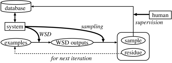
Figure 1: Flow of control of the example sampling system.

Several researchers have proposed this type of approach for NLP applications. Engelson and Dagan ([Engelson and Dagan, 1996] proposed a committee-based sampling method, which is currently applied to HMM training for part-of-speech tagging. This method sets several models (the committee) taken from a given supervised data set, and selects samples based on the degree of disagreement among the committee members as to the output. This method is implemented for statistics-based models. However, to formalize and map the concept of selective sampling into example-based approaches has yet to be explored.

Lewis and Gale ([Lewis and Gale, 1994] proposed an uncertainty sampling method for statistics-based text classification. In this method, the system always samples outputs with an uncertain level of correctness. In an example-based approach, we should take into account the training effect a given example has on other unsupervised examples. This is introduced as training utility in our method. We devote Section 4 to further comparison of our approach and other related works.

With respect to the problem of overhead for search, possible solutions would include the generalization of similar examples ([Kaji, Kida, and Morimoto, 1992, Nomiyama, 1993] or the reconstruction of the database using a small portion of useful instances selected from a given supervised example set ([Aha, Kibler, and Albert, 1991, Smyth and Keane, 1995]. However, such approaches imply a significant overhead for supervision of each example prior to the system’s execution. This shortcoming is precisely what our approach aims to avoid: we aim to reduce the overhead for supervision as well as the overhead for search.

Section 2 describes the basis of our verb sense disambiguation system and preliminary experiment, in which we compared our method with other disambiguation methods. Section 3 then elaborates on our example sampling method. Section 4 reports on the results of our experiments through comparison with other proposed selective sampling methods, and discusses theoretical differences between those methods.

2 Example-Based Verb Sense Disambiguation System

2.1 The Basic Idea

Our verb sense disambiguation system is based on the method proposed by Kurohashi and Nagao ([Kurohashi and Nagao, 1994] and later enhanced by Fujii et al. ([Fujii et al., 1996]. The system uses a database containing examples of collocations for each verb sense and its associated case frame(s). Figure 2 shows a fragment of the entry associated with the Japanese verb toru. The verb toru has multiple senses, a sample of which are ‘to take/steal,’ ‘to attain,’ ‘to subscribe,’ and ‘to reserve.’ The database specifies the case frame(s) associated with each verb sense. In Japanese, a complement of a verb consists of a noun phrase (case filler) and its case marker suffix, for example ga (nominative) or wo (accusative). The database lists several case filler examples for each case. The task of the system is to “interpret” the verbs occurring in the input text, i.e., to choose one sense from among a set of candidates. All verb senses we use are defined in IPAL ([Information-technology Promotion Agency, 1987], a machine-readable dictionary. IPAL also contains example case fillers as shown in Figure 2. Given an input, which is currently limited to a simple sentence, the system identifies the verb sense on the basis of the scored similarity between the input and the examples given for each verb sense. Let us take the sentence below as an example input:

• hisho ga	shindaisha wo	toru.
  (secretary-NOM)	(sleeping car-ACC)	(?)

In this example, one may consider hisho (‘secretary’) and shindaisha (‘sleeping car’) to be semantically similar to joshu (‘assistant’) and hikouki (‘airplane’) respectively, and since both collocate with the ‘to reserve’ sense of toru, one could infer that toru should be interpreted as ‘to reserve.’ This resolution originates from the analogy principle ([Nagao, 1984], and can be called nearest neighbor resolution because the verb in the input is disambiguated by superimposing the sense of the verb appearing in the example of highest similarity. The similarity between an input and an example is estimated based on the similarity between case fillers marked with the same case.

toru:
$\left\{\begin{tabular}[]{ll}{\it suri}\/&(pickpocket)\\ {\it kanojo}\/&(she)\\ {\it ani}\/&(brother)\end{tabular}\right\}$ ga	$\left\{\begin{tabular}[]{ll}{\it kane}\/&(money)\\ {\it saifu}\/&(wallet)\\ {\it otoko}\/&(man)\\ {\it uma}\/&(horse)\\ {\it aidea}\/&(idea)\end{tabular}\right\}$ wo	toru (to take/steal)
$\left\{\begin{tabular}[]{ll}{\it kare}\/&(he)\\ {\it kanojo}\/&(she)\\ {\it gakusei}\/&(student)\end{tabular}\right\}$ ga	$\left\{\begin{tabular}[]{ll}{\it menkyoshou}\/&(license)\\ {\it shikaku}\/&(qualification)\\ {\it biza}\/&(visa)\end{tabular}\right\}$ wo	toru (to attain)
$\left\{\begin{tabular}[]{ll}{\it kare}\/&(he)\\ {\it chichi}\/&(father)\\ {\it kyaku}\/&(client)\end{tabular}\right\}$ ga	$\left\{\begin{tabular}[]{ll}{\it shinbun}\/&(newspaper)\\ {\it zasshi}\/&(journal)\end{tabular}\right\}$ wo	toru (to subscribe)
$\left\{\begin{tabular}[]{ll}{\it kare}\/&(he)\\ {\it dantai}\/&(group)\\ {\it ryokoukyaku}\/&(passenger)\\ {\it joshu}\/&(assistant)\end{tabular}\right\}$ ga	$\left\{\begin{tabular}[]{ll}{\it kippu}\/&(ticket)\\ {\it heya}\/&(room)\\ {\it hikouki}\/&(airplane)\end{tabular}\right\}$ wo	toru (to reserve)
$\vdots$	$\vdots$	$\vdots$

Figure 2: A fragment of the database, and the entry associated with the Japanese verb toru.

Furthermore, since the restrictions imposed by the case fillers in choosing the verb sense are not equally selective, Fujii et al. ([Fujii et al., 1996] proposed a weighted case contribution to disambiguation (CCD) of the verb senses. This CCD factor is taken into account when computing the score for each sense of the verb in question. Consider again the case of toru in Figure 2. Since the semantic range of nouns collocating with the verb in the nominative does not seem to have a strong delinearization in a semantic sense (in Figure 2, the nominative of each verb sense displays the same general concept, i.e., HUMAN), it would be difficult, or even risky, to properly interpret the verb sense based on similarity in the nominative. In contrast, since the semantic ranges are disparate in the accusative, it would be feasible to rely more strongly on similarity here.

This argument can be illustrated as in Figure 3, in which the symbols $e_{1}$ and $e_{2}$ denote example case fillers of different case frames, and an input sentence includes two case fillers denoted by $x$ and $y$. The figure shows the distribution of example case fillers for the respective case frames, denoted in a semantic space. The semantic similarity between two given case fillers is represented by the physical distance between the two symbols. In the nominative, since $x$ happens to be much closer to an $e_{2}$ than any $e_{1}$, $x$ may be estimated to belong to the range of $e_{2}$’s, although $x$ actually belongs to both sets of $e_{1}$’s and $e_{2}$’s. In the accusative, however, $y$ would be properly estimated to belong to the set of $e_{1}$’s due to the disjunction of the two accusative case filler sets, even though examples do not fully cover each of the ranges of $e_{1}$’s and $e_{2}$’s. Note that this difference would be critical if example data were sparse. We will explain the method used to compute CCD in Section 2.2.

Figure 3: The semantic ranges of the nominative and accusative for the verb toru.

2.2 Methodology

To illustrate the overall algorithm, we will consider an abstract specification of both an input and the database (Figure 4). Let the input be {$n_{\mbox{$c_{1}$}}$–$m_{\mbox{$c_{1}$}}$, $n_{\mbox{$c_{2}$}}$–$m_{\mbox{$c_{2}$}}$, $n_{\mbox{$c_{3}$}}$–$m_{\mbox{$c_{3}$}}$, $v$}, where $n_{\mbox{$c_{i}$}}$ denotes the case filler for the case $c_{i}$, and $m_{\mbox{$c_{i}$}}$ denotes the case marker for $c_{i}$, and assume that the interpretation candidates for $v$ are derived from the database as $s_{1}$, $s_{2}$ and $s_{3}$. The database also contains a set ${\cal E}_{\mbox{$s_{i}$},\mbox{$c_{j}$}}$ of case filler examples for each case $c_{j}$ of each sense $s_{i}$ (“—” indicates that the corresponding case is not allowed).

input	$n_{\mbox{$c_{1}$}}$-$m_{\mbox{$c_{1}$}}$	$n_{\mbox{$c_{2}$}}$-$m_{\mbox{$c_{2}$}}$	$n_{\mbox{$c_{3}$}}$-$m_{\mbox{$c_{3}$}}$		$\mbox{$v$}\>(?)$
	${\cal E}_{\mbox{$s_{1}$},\mbox{$c_{1}$}}$	${\cal E}_{\mbox{$s_{1}$},\mbox{$c_{2}$}}$	${\cal E}_{\mbox{$s_{1}$},\mbox{$c_{3}$}}$	—	$\mbox{$v$}\>(\mbox{$s_{1}$}$)
database	${\cal E}_{\mbox{$s_{2}$},\mbox{$c_{1}$}}$	${\cal E}_{\mbox{$s_{2}$},\mbox{$c_{2}$}}$	${\cal E}_{\mbox{$s_{2}$},\mbox{$c_{3}$}}$	${\cal E}_{\mbox{$s_{2}$},\mbox{$c_{4}$}}$	$\mbox{$v$}\>(\mbox{$s_{2}$}$)
	—	${\cal E}_{\mbox{$s_{3}$},\mbox{$c_{2}$}}$	${\cal E}_{\mbox{$s_{3}$},\mbox{$c_{3}$}}$	—	$\mbox{$v$}\>(\mbox{$s_{3}$}$)

Figure 4: An input and the database.

During the verb sense disambiguation process, the system first discards those candidates whose case frame does not fit the input. In the case of Figure 4, $s_{3}$ is discarded because the case frame of $\mbox{$v$}\>(\mbox{$s_{3}$}$) does not subcategorize for the case $c_{1}$.

In the next step the system computes the score of the remaining candidates and chooses as the most plausible interpretation the one with the highest score. The score of an interpretation is computed by considering the weighted average of the similarity degrees of the input case fillers with respect to each of the example case fillers (in the corresponding case) listed in the database for the sense under evaluation. Formally, this is expressed by Equation (1), where $Score(\SS)$ is the score of sense $\SS$ of the input verb, and $SIM(\mbox{$n_{\mbox{$c$}}$},\mbox{${\cal E}_{\SS,\mbox{$c$}}$})$ is the maximum similarity degree between the input case filler $n_{\mbox{$c$}}$ and the corresponding case fillers in the database example set ${\cal E}_{\SS,\mbox{$c$}}$ (calculated through Equation (2)). $CCD(\mbox{$c$})$ is the weight factor of case $c$, which we will explain later in this section.

$$Score(\SS)=\frac{\textstyle\sum_{\mbox{$c$}}SIM(\mbox{$n_{\mbox{$c$}}$},\mbox{${\cal E}_{\SS,\mbox{$c$}}$})\cdot CCD(\mbox{$c$})}{\textstyle\sum_{\mbox{$c$}}CCD(\mbox{$c$})}$$ (1)

$$SIM(\mbox{$n_{\mbox{$c$}}$},\mbox{${\cal E}_{\SS,\mbox{$c$}}$})={\displaystyle\max_{\mbox{$e$}\in\mbox{${\cal E}_{\SS,\mbox{$c$}}$}}}sim(\mbox{$n_{\mbox{$c$}}$},\mbox{$e$})$$ (2)

 

Table 1: The relation between the length of the path between two nouns $n_{1}$ and $n_{2}$ in the Bunruigoihyo thesaurus ($len(n_{1},n_{2})$), and their relative similarity ($sim(n_{1},n_{2})$).

  $len(n_{1},n_{2})$ 0 2 4 6 8 10 12 $sim(n_{1},n_{2})$ 11 10 9 8 7 5 0

With regard to the computation of the similarity between two different case fillers ($sim(\mbox{$n_{\mbox{$c$}}$},\mbox{$e$})$ in Equation (1)), we experimentally used two alternative approaches. The first approach uses semantic resources, that is, hand-crafted thesauri (such as the Roget’s thesaurus ([Chapman, 1984] or WordNet ([Miller et al., 1993] in the case of English, and Bunruigoihyo ([National Language Research Institute, 1964] or EDR ([Japan Electronic Dictionary Research Institute, 1995] in the case of Japanese), based on the intuitively feasible assumption that words located near each other within the structure of a thesaurus have similar meaning. Therefore, the similarity between two given words is represented by the length of the path between them in the thesaurus structure ([Fujii et al., 1996, Kurohashi and Nagao, 1994, Li, Szpakowicz, and Matwin, 1995, Uramoto, 1994b]. We used the similarity function empirically identified by Kurohashi and Nagao in which the relation between the length of the path in the Bunruigoihyo thesaurus and the similarity between words is defined as shown in Table 1. In this thesaurus, each entry is assigned a seven-digit class code. In other words, this thesaurus can be considered as a tree, seven levels in depth, with each leaf as a set of words. Figure 5 shows a fragment of the Bunruigoihyo thesaurus including some of the nouns in both Figure 2 and the input sentence above.

The second approach is based on statistical modeling. We adopted one typical implementation called the “vector space model” (VSM) ([Frakes and Baeza-Yates, 1992, Leacock, Towell, and Voorhees, 1993, Salton and McGill, 1983, Schütze, 1992], which has a long history of application in information retrieval (IR) and text categorization (TC) tasks. In the case of IR/TC, VSM is used to compute the similarity between documents, which is represented by a vector comprising statistical factors of content words in a document. Similarly, in our case, each noun is represented by a vector comprising statistical factors, although statistical factors are calculated in terms of the predicate-argument structure in which each noun appears. Predicate-argument structures, which consist of complements (case filler nouns and case markers) and verbs, have also been used in the task of noun classification ([Hindle, 1990]. This can be expressed by Equation (3), where $\vec{n}$ is the vector for the noun in question, and items $t_{i}$ represent the statistics for predicate-argument structures including $n$.

$$\vec{n}=<t_{1},~{}t_{2},~{}\ldots,~{}t_{i},~{}\ldots>$$ (3)

In regard to $t_{i}$, we used the notion of TF$\cdot$IDF ([Salton and McGill, 1983]. TF (term frequency) gives each context (a case marker/verb pair) importance proportional to the number of times it occurs with a given noun. The rationale behind IDF (inverse document frequency) is that contexts which rarely occur over collections of nouns are valuable, and that therefore the IDF of a context is inversely proportional to the number of noun types that appear in that context. This notion is expressed by Equation (4), where $f(<\!n,c,v\!>)$ is the frequency of the tuple $<\!n,c,v\!>$, $nf(<\!c,v\!>)$ is the number of noun types which collocate with verb $v$ in the case $c$, and $N$ is the number of noun types within the overall co-occurrence data.

$$t_{i}=f(<\!n,c,v\!>)\cdot\log\frac{\textstyle N}{\textstyle nf(<\!c,v\!>)}$$ (4)

We then compute the similarity between nouns $n_{1}$ and $n_{2}$ by the cosine of the angle between the two vectors $\vec{n_{1}}$ and $\vec{n_{2}}$. This is realized by Equation (5).

$$sim(n_{1},n_{2})=\frac{\textstyle\vec{n_{1}}\cdot\vec{n_{2}}}{\textstyle|\vec{n_{1}}||\vec{n_{2}}|}$$ (5)

We extracted co-occurrence data from the RWC text base RWC-DB-TEXT-95-1 ([Real World Computing Partnership, 1995]. This text base consists of four years worth of Mainichi Shimbun newspaper articles ([Mainichi Shimbun, 1991-1994], which have been automatically annotated with morphological tags. The total morpheme content is about one hundred million. Since full parsing is usually expensive, a simple heuristic rule was used to obtain collocations of nouns, case markers, and verbs in the form of tuples $<\!n,c,v\!>$. This rule systematically associates each sequence of noun and case marker to the verb of highest proximity, and produced 419,132 tuples. This co-occurrence data was used in the preliminary experiment described in Section 2.3.

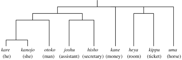
Figure 5: A fragment of the Bunruigoihyo thesaurus.

In Equation (1), $CCD(\mbox{$c$})$ expresses the weight factor of the contribution of case $c$ to (current) verb sense disambiguation. Intuitively, preference should be given to cases displaying case fillers that are classified in semantic categories of greater disjunction. Thus, $c$’s contribution to the sense disambiguation of a given verb, $CCD(\mbox{$c$})$, is likely to be higher if the example case filler sets {$\mbox{${\cal E}_{\mbox{$s_{i}$},\mbox{$c$}}$}~{}|~{}i=1,\ldots,n$} share fewer elements as in Equation (6).

$$\begin{array}[]{l}CCD(\mbox{$c$})={\displaystyle\left(\frac{\displaystyle 1}{{}_{\it n\/}{\rm C}_{2}}\sum_{{\it i\/}=1}^{{\it n\/}-1}\sum_{{\it j\/}={\it i\/}+1}^{{\it n\/}}\frac{\displaystyle|\mbox{${\cal E}_{\mbox{$s_{i}$},\mbox{$c$}}$}|+|\mbox{${\cal E}_{\mbox{$s_{j}$},\mbox{$c$}}$}|-2|\mbox{${\cal E}_{\mbox{$s_{i}$},\mbox{$c$}}$}\cap\mbox{${\cal E}_{\mbox{$s_{j}$},\mbox{$c$}}$}|}{\displaystyle|\mbox{${\cal E}_{\mbox{$s_{i}$},\mbox{$c$}}$}|+|\mbox{${\cal E}_{\mbox{$s_{j}$},\mbox{$c$}}$}|}\right)^{\alpha}}\end{array}$$ (6)

Here, $\alpha$ is a constant for parameterizing the extent to which CCD influences verb sense disambiguation. The larger $\alpha$, the stronger CCD’s influence on the system output. To avoid data sparseness, we smooth each element (noun example) in ${\cal E}_{\mbox{$s_{i}$},\mbox{$c$}}$. In practice, this involves generalizing each example noun into a five-digit class based on the Bunruigoihyo thesaurus, as has been commonly used for smoothing.

2.3 Preliminary Experimentation

We estimated the performance of our verb sense disambiguation method through an experiment, in which we compared the following five methods:

• lower bound (LB), in which the system systematically chooses the most frequently appearing verb sense in the database ([Gale, Church, and Yarowsky, 1992],

• rule-based method (RB), in which the system uses a thesaurus to (automatically) identify appropriate semantic classes as selectional restrictions for each verb complement,

• Naive-Bayes method (NB), in which the system interprets a given verb based on the probability that it takes each verb sense,

• example-based method using the vector space model (VSM), in which the system uses the above mentioned co-occurrence data extracted from the RWC text base,

• example-based method using the Bunruigoihyo thesaurus (BGH), in which the system uses Table 1 for the similarity computation.

In the rule-based method, the selectional restrictions are represented by thesaurus classes, and allow only those nouns dominated by the given class in the thesaurus structure as verb complements. In order to identify appropriate thesaurus classes, we used the association measure proposed by Resnik ([Resnik, 1993], which computes the information-theoretic association degree between case fillers and thesaurus classes, for each verb sense (Equation (7)).

$$A(\SS,\mbox{$c$},r)=P(r|\SS,\mbox{$c$})\cdot\log\frac{\textstyle P(r|\SS,\mbox{$c$})}{\textstyle P(r|\mbox{$c$})}$$ (7)

Here, $A(\SS,\mbox{$c$},r)$ is the association degree between verb sense $\SS$ and class $r$ (selectional restriction candidate) with respect to case $c$. $P(r|\SS,\mbox{$c$})$ is the conditional probability that a case filler example associated with case $c$ of sense $\SS$ is dominated by class $r$ in the thesaurus. $P(r|\mbox{$c$})$ is the conditional probability that a case filler example for case $c$ (disregarding verb sense) is dominated by class $r$. Each probability is estimated based on training data. We used the semantic classes defined in the Bunruigoihyo thesaurus. In practice, every $r$ whose association degree is above a certain threshold is chosen as a selectional restriction ([Resnik, 1993, Ribas, 1995]. By decreasing the value of the threshold, system coverage can be broadened, but this opens the way for irrelevant (noisy) selectional rules.

The Naive-Bayes method assumes that each case filler included in a given input is conditionally independent of other case fillers: the system approximates the probability that an input $x$ takes a verb sense $\SS$ ($P(\SS|x)$), simply by computing the product of the probability that each verb sense $\SS$ takes $n_{\mbox{$c$}}$ as a case filler for case $c$. The verb sense with maximal probability is then selected as the interpretation (Equation (8)).

$$\begin{array}[]{lll}{\displaystyle\arg\max_{\SS}P(\SS|x)}&=&{\displaystyle\arg\max_{\SS}\frac{\textstyle P(\SS)\cdot P(x|\SS)}{\textstyle P(x)}}\\ \vskip 4.30554pt\cr&=&{\displaystyle\arg\max_{\SS}P(\SS)\cdot P(x|\SS)}\\ \vskip 4.30554pt\cr&\approx&{\displaystyle\arg\max_{\SS}P(\SS)\prod_{\mbox{$c$}}P(\mbox{$n_{\mbox{$c$}}$}|\SS)}\end{array}$$ (8)

Here, $P(\mbox{$n_{\mbox{$c$}}$}|\SS)$ is the probability that a case filler associated with sense $\SS$ for case $c$ in the training data is $n_{\mbox{$c$}}$. We estimated $P(\SS)$ based on the distribution of the verb senses in the training data. In practice, data sparseness leads to not all case fillers $n_{\mbox{$c$}}$ appearing in the database, and as such, we generalize each $n_{\mbox{$c$}}$ into semantic class defined in the Bunruigoihyo thesaurus.

All methods excepting the lower bound method involve a parametric constant: the threshold value for the association degree (RB), a generalization level for case filler nouns (NB), and $\alpha$ in Equation (6) (VSM and BGH). For these parameters, we conducted several trials prior to the actual comparative experiment, to determine the optimal parameter values over a range of data sets. For our method, we set $\alpha$ extremely large, which is equivalent to relying almost solely on the SIM of the case with greatest CCD. However, note that when the SIM of the case with greatest CCD is equal for multiple verb senses, the system computes the SIM of the case with second highest CCD. This process is repeated until only one verb sense remains. When more than one verb sense is selected for any given method (or none of them remains, for the rule-based method), the system simply selects the verb sense that appears most frequently in the database.

In the experiment, we conducted sixfold cross-validation, that is, we divided the training/test data into six equal parts, and conducted six trials in which a different part was used as test data each time, and the rest as training data (the database). We evaluated the performance of each method according to its accuracy, that is the ratio of the number of correct outputs compared to the total number of inputs. The training/test data used in the experiment contained about one thousand simple Japanese sentences collected from news articles. Each sentence in the training/test data contained one or more complement(s) followed by one of the eleven verbs described in Table 2. In Table 2, the column of “English Gloss” describes typical English translations of the Japanese verbs. The column of “# of Sentences” denotes the number of sentences in the corpus, and “# of Senses” denotes the number of verb senses contained in IPAL. The column of “Accuracy” shows the accuracy of each method.

 

Table 2: The verbs contained in the corpus used, and the accuracy of the different verb sense disambiguation methods (LB: lower bound, RB: rule-based method, NB: Naive-Bayes method, VSM: vector space model, BGH: the Bunruigoihyo thesaurus).

  # of # of Accuracy (%) Verb English Gloss Sentences Senses LB RB NB VSM BGH ataeru give 136 4  66.9  62.1  75.8  84.1  86.0 kakeru hang 160 29 25.6 24.6 67.6 73.4 76.2 kuwaeru add 167 5 53.9 65.6 82.2 84.0 86.8 motomeru require 204 4 85.3 82.4 87.0 85.5 85.5 noru ride 126 10 45.2 52.8 81.4 80.5 85.3 osameru govern 108 8 30.6 45.6 66.0 72.0 74.5 tsukuru make 126 15 25.4 24.9 59.1 56.5 69.9 toru take 84 29 26.2 16.2 56.1 71.2 75.9 umu bear offspring 90 2 83.3 94.7 95.5 92.0 99.4 wakaru understand 60 5 48.3 40.6 71.4 62.5 70.7 yameru stop 54 2 59.3 89.9 92.3 96.2 96.3 total — 1,315 — 51.4 54.8 76.6 78.6 82.3

Looking at Table 2, one can see that our example-based method performed better than the other methods (irrespective of the similarity computation), although the Naive-Bayes method is relatively comparable in performance. Surprisingly, despite the relatively ad hoc similarity definition utilized (see Table 1), the Bunruigoihyo thesaurus led to a greater accuracy gain than the vector space model. In order to estimate the upper bound (limitation) of the disambiguation task, that is, to what extent a human expert makes errors in disambiguation ([Gale, Church, and Yarowsky, 1992], we analyzed incorrect outputs and found that roughly 30% of the system errors using the Bunruigoihyo thesaurus fell into this category. It should be noted that while the vector space model requires computational cost (time/memory) of an order proportional to the size of the vector, determination of paths in the Bunruigoihyo thesaurus comprises a trivial cost.

We also investigated errors made by the rule-based method to find a rational explanation for its inferiority. We found that the association measure in Equation (7) tends to give a greater value to less frequently appearing verb senses and lower level (more specified) classes, and therefore chosen rules are generally overspecified. Consequently, frequently appearing verb senses are likely to be rejected. On the other hand, when attempting to enhance the rule set by setting a smaller threshold value for the association score, overgeneralization can be a problem. We also note that one of the theoretical differences between the rule-based and example-based methods is that the former statically generalizes examples (prior to system usage), while the latter does so dynamically. Static generalization would appear to be relatively risky for sparse training data.

Although comparison of different approaches to word sense disambiguation should be further investigated, this experimental result gives us good motivation to explore example-based verb sense disambiguation approaches, i.e., to introduce the notion of selective sampling into them.

2.4 Enhancement of Verb Sense Disambiguation

Let us discuss how further enhancements to our example-based verb sense disambiguation system could be made. First, since inputs are simple sentences, information for word sense disambiguation is inadequate in some cases. External information such as the discourse or domain dependency of each word sense ([Guthrie et al., 1991, Nasukawa, 1993, Yarowsky, 1995] is expected to lead to system improvement. Second, some idiomatic expressions represent highly restricted collocations, and overgeneralizing them semantically through the use of a thesaurus can cause further errors. Possible solutions would include one proposed by Uramoto, in which idiomatic expressions are described separately in the database so that the system can control their overgeneralization ([Uramoto, 1994b]. Third, a number of existing NLP tools such as the JUMAN (morphological analyzer) ([Matsumoto et al., 1993] and QJP (morphological and syntactic analyzer) ([Kameda, 1996] could broaden the coverage of our system, as inputs are currently limited to simple, morphologically analyzed sentences. Finally, it should be noted that in Japanese, case markers can be omitted or topicalized (for example, marked with postposition wa), an issue which our framework does not currently consider.

3 Example Sampling Algorithm

3.1 Overview

Let us look again at Figure 1 in Section 1. In this figure, “WSD outputs” refers to a corpus in which each sentence is assigned an expected verb interpretation during the WSD phase. In the training phase, the system stores supervised samples (with each interpretation simply checked or appropriately corrected by a human) in the database, to be used in a later WSD phase. In this section, we turn to the problem as to which examples should be selected as samples.

Lewis and Gale ([Lewis and Gale, 1994] proposed the notion of uncertainty sampling for the training of statistics-based text classifiers. Their method selects those examples that the system classifies with minimum certainty, based on the assumption that there is no need for teaching the system the correct answer when it has answered with sufficiently high certainty. However, we should take into account the training effect a given example has on other remaining (unsupervised) examples. In other words, we would like to select samples such as to be able to correctly disambiguate as many examples as possible in the next iteration. If this is successfully done, the number of examples to be supervised will decrease. We consider maximization of this effect by means of a training utility function aimed at ensuring that the most useful example at a given point in time is the example with the greatest training utility factor. Intuitively speaking, the training utility of an example is greater when we can expect greater increase in the interpretation certainty of the remaining examples after training using that example.

To explain this notion intuitively, let us take Figure 6 as an example corpus. In this corpus, all sentences contain the verb yameru, which has two senses according to IPAL, $s_{1}$ (‘to stop (something)’) and $s_{2}$ (‘to quit (occupation)’). In this figure, sentences $e_{1}$ and $e_{2}$ are supervised examples associated with the senses $s_{1}$ and $s_{2}$, respectively, and $x_{i}$’s are unsupervised examples. For the sake of enhanced readability, the examples $x_{i}$’s are partitioned according to their verb senses, that is, $x_{1}$ to $x_{5}$ correspond to sense $s_{1}$, and $x_{6}$ to $x_{9}$ correspond to sense $s_{2}$. In addition, note that examples in the corpus can be readily categorized based on case similarity, that is, into clusters $\{x_{1},x_{2},x_{3},x_{4}\}$ (‘someone/something stops service’), $\{e_{2},x_{6},x_{7}\}$ (‘someone leaves organization’), $\{x_{8},x_{9}\}$ (‘someone quits occupation’), $\{e_{1}\}$, and $\{x_{5}\}$. Let us simulate the sampling procedure with this example corpus. In the initial stage with $\{e_{1},e_{2}\}$ in the database, $x_{6}$ and $x_{7}$ can be interpreted as $s_{2}$ with greater certainty than for other $x_{i}$’s, because these two examples are similar to $e_{2}$. Therefore, uncertainty sampling selects any example excepting $x_{6}$ and $x_{7}$ as the sample. However, any one of examples $x_{1}$ to $x_{4}$ is more desirable because by way of incorporating one of these examples, we can obtain more $x_{i}$’s with greater certainty. Assuming that $x_{1}$ is selected as the sample and incorporated into the database with sense $s_{1}$, either of $x_{8}$ and $x_{9}$ will be more highly desirable than other unsupervised $x_{i}$’s in the next stage.

$e_{1}$:	seito ga (student-NOM)	shitsumon wo (question-ACC)	yameru ($s_{1}$)
$e_{2}$:	ani ga (brother-NOM)	kaisha wo (company-ACC)	yameru ($s_{2}$)
$x_{1}$:	shain ga (employee-NOM)	eigyou wo (sales-ACC)	yameru (?)
$x_{2}$:	shouten ga (store-NOM)	eigyou wo (sales-ACC)	yameru (?)
$x_{3}$:	koujou ga (factory-NOM)	sougyou wo (operation-ACC)	yameru (?)
$x_{4}$:	shisetsu ga (facility-NOM)	unten wo (operation-ACC)	yameru (?)
$x_{5}$:	sensyu ga (athlete-NOM)	renshuu wo (practice-ACC)	yameru (?)
$x_{6}$:	musuko ga (son-NOM)	kaisha wo (company-ACC)	yameru (?)
$x_{7}$:	kangofu ga (nurse-NOM)	byouin wo (hospital-ACC)	yameru (?)
$x_{8}$:	hikoku ga (defendant-NOM)	giin wo (congressman-ACC)	yameru (?)
$x_{9}$:	chichi ga (father-NOM)	kyoushi wo (teacher-ACC)	yameru (?)

Figure 6: Example of a given corpus associated with the verb yameru.

Let S be a set of sentences, i.e., a given corpus, and D be the subset of supervised examples stored in the database. Further, let X be the set of unsupervised examples, realizing Equation (9).

$$\mbox{\bf S}=\mbox{\bf D}\cup\mbox{\bf X}$$ (9)

The example sampling procedure can be illustrated as:

1. $WSD(\mbox{\bf D},\mbox{\bf X})$

2. $e\leftarrow\arg\max_{x\in\mbox{\bf X}}TU(x)$

3. $\mbox{\bf D}\leftarrow\mbox{\bf D}\cup\{e\},~{}~{}\mbox{\bf X}\leftarrow\mbox{\bf X}\cap\overline{\{e\}}$

4. goto 1

where $WSD(\mbox{\bf D},\mbox{\bf X})$ is the verb sense disambiguation process on input X using D as the database. In this disambiguation process, the system outputs the following for each input: (a) a set of verb sense candidates with interpretation scores, and (b) an interpretation certainty. These factors are used for the computation of $TU(x)$, newly introduced in our method. $TU(x)$ computes the training utility factor for an example $x$. The sampling algorithm gives preference to examples of maximum utility.

We will explain in the following sections how $TU(x)$ is estimated, based on the estimation of the interpretation certainty.

3.2 Interpretation Certainty

Lewis and Gale ([Lewis and Gale, 1994] estimate certainty of an interpretation as the ratio between the probability of the most plausible text category and the probability of any other text category, excluding the most probable one. Similarly, in our verb sense disambiguation system, we introduce the notion of interpretation certainty of examples based on the following preference conditions:

1. the highest interpretation score is greater,

2. the difference between the highest and second highest interpretation scores is greater.

The rationale for these conditions is given below. Consider Figure 7, where each symbol denotes an example in a given corpus, with symbols $x$ as unsupervised examples and symbols $e$ as supervised examples. The curved lines delimit the semantic vicinities (extents) of the two verb senses 1 and 2, respectively. The semantic similarity between two examples is graphically portrayed by the physical distance between the two symbols representing them. In Figure 7(a), $x$’s located inside a semantic vicinity are expected to be interpreted as being similar to the appropriate example $e$ with high certainty, a fact which is in line with condition 1 above. However, in Figure 7(b), the degree of certainty for the interpretation of any $x$ located inside the intersection of the two semantic vicinities cannot be great. This occurs when the case fillers associated with two or more verb senses are not selective enough to allow for a clear-cut delineation between them. This situation is explicitly rejected by condition 2.

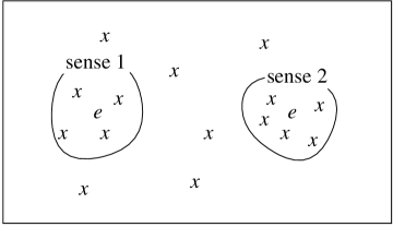
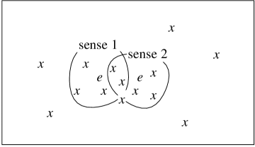
(a) (b)

Figure 7: The concept of interpretation certainty. The case where the interpretation certainty of the enclosed $x$’s is great is shown in (a). The case where the interpretation certainty of the $x$’s contained in the intersection of senses 1 and 2 is small is shown in (b).

Based on the above two conditions, we compute interpretation certainties using Equation (10), where $C(x)$ is the interpretation certainty of an example $x$. $Score_{1}(x)$ and $Score_{2}(x)$ are the highest and second highest scores for $x$, respectively, and $\lambda$, which ranges from 0 to 1, is a parametric constant used to control the degree to which each condition affects the computation of $C(x)$.

$$C(x)=\lambda\cdot Score_{1}(x)+(1-\lambda)\cdot(Score_{1}(x)-Score_{2}(x))$$ (10)

Through a preliminary experiment, we estimated the validity of the notion of the interpretation certainty, by the trade-off between accuracy and coverage of the system. Note that in this experiment, accuracy is the ratio of the number of correct outputs and the number of cases where the interpretation certainty of the output is above a certain threshold. Coverage is the ratio of the number of cases where the interpretation certainty of the output is above a certain threshold and the number of inputs. By raising the value of the threshold, accuracy also increases (at least theoretically), while coverage decreases.

The system used the Bunruigoihyo thesaurus for the similarity computation, and was evaluated by way of sixfold cross-validation using the same corpus as that used for the experiment described in Section 2.3. Figure 8 shows the result of the experiment with several values of $\lambda$, from which the optimal $\lambda$ value seems to be in the range around 0.5. It can be seen that, as we assumed, both of the above conditions are essential for the estimation of the interpretation certainty.

Figure 8: The relation between coverage and accuracy with different $\lambda$’s.

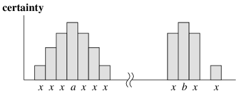
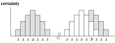
(a) (b)

Figure 9: The concept of training utility. The case where the training utility of $a$ is greater than that of $b$ because $a$ has more unsupervised neighbors is shown in (a); (b) shows the case where the training utility of $a$ is greater than that of $b$ because $b$ closely neighbors $e$, contained in the database.

3.3 Training Utility

The training utility of an example $a$ is greater than that of another example $b$ when the total interpretation certainty of unsupervised examples increases more after training with example $a$ than with example $b$. Let us consider Figure 9, in which the x-axis mono-dimensionally denotes the semantic similarity between two unsupervised examples, and the y-axis denotes the interpretation certainty of each example. Let us compare the training utility of the examples $a$ and $b$ in Figure 9(a). Note that in this figure, whichever example we use for training, the interpretation certainty for each unsupervised example ($x$) neighboring the chosen example increases based on its similarity to the supervised example. Since the increase in the interpretation certainty of a given $x$ becomes smaller as the similarity to $a$ or $b$ diminishes, the training utility of the two examples can be represented by the shaded areas. The training utility of $a$ is greater as it has more neighbors than $b$. On the other hand, in Figure 9(b), $b$ has more neighbors than $a$. However, since $b$ is semantically similar to $e$, which is already contained in the database, the total increase in interpretation certainty of its neighbors, i.e., the training utility of $b$, is smaller than that of $a$.

Let $\Delta C(x\!=\!\SS,y)$ be the difference in the interpretation certainty of $y\in\mbox{\bf X}$ after training with $x\in\mbox{\bf X}$, taken with the sense $\SS$. $TU(x\!=\!\SS)$, which is the training utility function for $x$ taken with sense $\SS$, can be computed by way of Equation (11).

$$TU(x\!=\!\SS)=\sum_{y\in\mbox{\bf X}}\Delta C(x\!=\!\SS,y)$$ (11)

It should be noted that in Equation (11), we can replace X with a subset of X which consists of neighbors of $x$. However, in order to facilitate this, an efficient algorithm to search for neighbors of an example is required. We will discuss this problem in Section 3.5.

Since there is no guarantee that $x$ will be supervised with any given sense $\SS$, it can be risky to rely solely on $TU(x\!=\!\SS)$ for the computation of $TU(x)$. We estimate $TU(x)$ by the expected value of $x$, calculating the average of each $TU(x\!=\!\SS)$, weighted by the probability that $x$ takes sense $\SS$. This can be realized by Equation (12), where $P(\SS|x)$ is the probability that $x$ takes the sense $\SS$.

$$TU(x)=\sum_{\SS}P(\SS|x)\cdot TU(x\!=\!\SS)$$ (12)

Given the fact that (a) $P(\SS|x)$ is difficult to estimate in the current formulation, and (b) the cost of computation for each $TU(x\!=\!\SS)$ is not trivial, we temporarily approximate $TU(x)$ as in Equation (13), where K is a set of the $k$-best verb sense(s) of $x$ with respect to the interpretation score in the current state.

$$TU(x)\approx\frac{\textstyle 1}{\textstyle k}\sum_{\SS\in\mbox{\bf K}}TU(x\!=\!\SS)$$ (13)

3.4 Enhancement of computation

In this section, we discuss how to enhance the computation associated with our example sampling algorithm.

First, we note that computation of $TU(x\!=\!\SS)$ in Equation (11) above becomes time consuming because the system is required to search the whole set of unsupervised examples for examples whose interpretation certainty will increase after $x$ is used for training. To avoid this problem, we could potentially apply a method used in efficient database search techniques, by which the system can search for neighbor examples of $x$ with optimal time complexity ([Utsuro et al., 1994]. However, in this section, we will explain another efficient algorithm to identify neighbors of $x$, in which neighbors of case fillers are considered to be given directly by the thesaurus structure. The basic idea is the following: the system searches for neighbors of each case filler of $x$ instead of $x$ as a whole, and merges them as a set of neighbors of $x$. Note that by dividing examples along the lines of each case filler, we can retrieve neighbors based on the structure of the Bunruigoihyo thesaurus (instead of the conceptual semantic space as in Figure 7). Let $\mbox{\bf N}_{x=\SS,\mbox{$c$}}$ be a subset of unsupervised neighbors of $x$ whose interpretation certainty will increase after $x$ is used for training, considering only case $c$ of sense $\SS$. The actual neighbor set of $x$ with sense $\SS$ ($\mbox{\bf N}_{x=\SS}$) is then defined as in Equation (14).

$$\mbox{$\mbox{\bf N}_{x=\SS}$}=\bigcup_{\mbox{$c$}}\mbox{$\mbox{\bf N}_{x=\SS,\mbox{$c$}}$}$$ (14)

Figure 10 shows a fragment of the thesaurus, in which $x$ and the $y$’s are unsupervised case filler examples. Symbols $e_{1}$ and $e_{2}$ are case filler examples stored in the database taken as senses $s_{1}$ and $s_{2}$, respectively. The triangles represent subtrees of the structure, and the labels $n_{i}$ represent nodes. In this figure, it can easily be seen that the interpretation score of $s_{1}$ never changes for examples other than the children of $n_{4}$, after $x$ is used for training with sense $s_{1}$. In addition, incorporating $x$ into the database with sense $s_{1}$ never changes the score of examples $y$ for other sense candidates. Therefore, $\mbox{\bf N}_{x=\mbox{$s_{1}$},\mbox{$c$}}$ includes only examples dominated by $n_{4}$, in other words, examples that are more closer to $x$ than $e_{1}$ in the thesaurus structure. Since, during the WSD phase, the system determines $e_{1}$ as the supervised neighbor of $x$ for sense $s_{1}$, identifying $\mbox{\bf N}_{x=\mbox{$s_{1}$},\mbox{$c$}}$ does not require any extra computational overhead. We should point out that the technique presented here is not applicable when the vector space model (see Section 2.2) is used for the similarity computation. However, automatic clustering algorithms, which assign a hierarchy to a set of words based on the similarity between them (for example the one proposed by Tokunaga, Iwayama, and Tanaka ([Tokunaga, Iwayama, and Tanaka, 1995]), could potentially facilitate the application of this retrieval method to the vector space model.

                                $n_{1}$ $n_{2}$ $n_{3}$                      

Figure 10: A fragment of the thesaurus including neighbors of $x$ associated with case $c$.

Second, sample size at each iteration should ideally be one, so as to avoid the supervision of similar examples. On the other hand, a small sampling size generates a considerable computation overhead for each iteration of the sampling procedure. This can be a critical problem for statistics-based approaches, as the reconstruction of statistic classifiers is expensive. However, example-based systems fortunately do not require reconstruction, and examples simply have to be stored in the database. Furthermore, in each disambiguation phase, our example-based system needs only compute the similarity between each newly stored example and its unsupervised neighbors, rather than between every example in the database and every unsupervised example. Let us reconsider Figure 10. As mentioned above, when $x$ is stored in the database with sense $s_{1}$, only the interpretation score of $y$’s dominated by $n_{4}$, i.e., $\mbox{\bf N}_{x=\mbox{$s_{1}$},\mbox{$c$}}$, will be changed with respect to sense $s_{1}$. This algorithm reduces the time complexity of each iteration from $O(N^{2})$ to $O(N)$, given that $N$ is the total number of examples in a given corpus.

3.5 Discussion

3.5.1 Sense Ambiguity of Case Fillers in Selective Sampling

The semantic ambiguity of case fillers (nouns) should be taken into account during selective sampling. Figure 11, which uses the same basic notation as Figure 7, illustrates one possible problem caused by case filler ambiguity. Let $x_{1}$ be a sense of a case filler $x$, and $y_{1}$ and $y_{2}$ be different senses of a case filler $y$. On the basis of Equation (10), the interpretation certainty of $x$ and $y$ is small in Figures 11(a) and 11(b), respectively. However, in the situation shown in Figure 11(b), since (a) the task of distinguishing between the verb senses 1 and 2 is easier, and (b) instances where the sense ambiguity of case fillers corresponds to distinct verb senses will be rare, training using either $y_{1}$ or $y_{2}$ will be less effective than using a case filler of the type of $x$. It should also be noted that since Bunruigoihyo is a relatively small-sized thesaurus with limited word sense coverage, this problem is not critical in our case. However, given other existing thesauri like the EDR electronic dictionary ([Japan Electronic Dictionary Research Institute, 1995] or WordNet ([Miller et al., 1993], these two situations should be strictly differentiated.

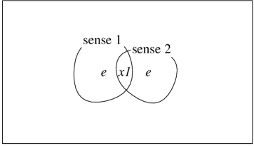
(a) (b)

Figure 11: Two separate scenarios in which the interpretation certainty of $x$ is small. In (a), interpretation certainty of $x$ is small because $x$ lies in the intersection of distinct verb senses; in (b), interpretation certainty of $y$ is small because $y$ is semantically ambiguous.

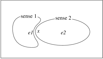
Figure 12: The case where informative example $x$ is not selected.

3.5.2 A Limitation of our Selective Sampling Method

Figure 12, where the basic notation is the same as in Figure 7, exemplifies a limitation of our sampling method. In this figure, the only supervised examples contained in the database are $e_{1}$ and $e_{2}$, and $x$ represents an unsupervised example belonging to sense 2. Given this scenario, $x$ is informative because (a) it clearly evidences the semantic vicinity of sense 2, and (b) without $x$ as sense 2 in the database, the system may misinterpret other examples neighboring $x$. However, in our current implementation, the training utility of $x$ would be small because it would be mistakenly interpreted as sense 1 with great certainty due to its relatively close semantic proximity to $e_{1}$. Even if $x$ has a number of unsupervised neighbors, the total increment of their interpretation certainty cannot be expected to be large. This shortcoming often presents itself when the semantic vicinities of different verb senses are closely aligned or their semantic ranges are not disjunctive. Here, let us consider Figure 3 again, in which the nominative case would parallel the semantic space shown in Figure 12 more closely than the accusative. Relying more on the similarity in the accusative (the case with greater CCD) as is done in our system, we aim to map the semantic space in such a way as to achieve higher semantic disparity and minimize this shortcoming.

4 Evaluation

4.1 Comparative Experimentation

In order to investigate the effectiveness of our example sampling method, we conducted an experiment, in which we compared the following four sampling methods:

• a control (random), in which a certain proportion of a given corpus is randomly selected for training,

• uncertainty sampling (US), in which examples with minimum interpretation certainty are selected ([Lewis and Gale, 1994],

• committee-based sampling (CBS) ([Engelson and Dagan, 1996],

• our method based on the notion of training utility (TU).

We elaborate on uncertainty sampling and committee-based sampling in Section 4.2. We compared these sampling methods by evaluating the relation between the number of training examples sampled and the performance of the system. We conducted sixfold cross-validation and carried out sampling on the training set. With regard to the training/test data set, we used the same corpus as that used for the experiment described in Section 2.3. Each sampling method uses examples from IPAL to initialize the system, with the number of example case fillers for each case being an average of about 3.7. For each sampling method, the system uses the Bunruigoihyo thesaurus for the similarity computation. In Table 2 (in Section 2.3), the column of “accuracy” for “BGH” denotes the accuracy of the system with the entire set of training data contained in the database. Each of the four sampling methods achieved this figure at the conclusion of training.

We evaluated each system performance according to its accuracy, that is the ratio of the number of correct outputs, compared to the total number of inputs. For the purpose of this experiment, we set the sample size to 1 for each iteration, $\lambda=0.5$ for Equation (10), and $k=1$ for Equation (13). Based on a preliminary experiment, increasing the value of $k$ either did not improve the performance over that for $k=1$, or lowered the overall performance. Figure 13 shows the relation between the number of the training data sampled and the accuracy of the system. In Figure 13, zero on the x-axis represents the system using only the examples provided by IPAL. Looking at Figure 13 one can see that compared with random sampling and committee-based sampling, our sampling method reduced the number of the training data required to achieve any given accuracy. For example, to achieve an accuracy of 80%, the number of the training data required for our method was roughly one-third of that for random sampling. Although the accuracy for our method was surpassed by that for uncertainty sampling for larger sizes of training data, this minimal difference for larger data sizes is overshadowed by the considerable performance gain attained by our method for smaller data sizes.

Since IPAL has, in a sense, been manually selectively sampled in an attempt to model the maximum verb sense coverage, the performance of each method is biased by the initial contents of the database. To counter this effect, we also conducted an experiment involving the construction of the database from scratch, without using examples from IPAL. During the initial phase, the system randomly selected one example for each verb sense from the training set, and a human expert provided the correct interpretation to initialize the system. Figure 14 shows the performance of the various methods, from which the same general tendency as seen in Figure 13 is observable. However, in this case, our method was generally superior to other methods. Through these comparative experiments, we can conclude that our example sampling method is able to decrease the number of the training data, i.e., the overhead for both supervision and searching, without degrading the system performance.

Figure 13: The relation between the number of training data sampled and accuracy of the system.

4.2 Related Work

4.2.1 Uncertainty Sampling

The procedure for uncertainty sampling ([Lewis and Gale, 1994] is as follows, where $C(x)$ represents the interpretation certainty for an example $x$ (see our sampling procedure in Section 3.1 for comparison):

1. $WSD(\mbox{\bf D},\mbox{\bf X})$

2. $e\leftarrow\arg\min_{x\in\mbox{\bf X}}C(x)$

3. $\mbox{\bf D}\leftarrow\mbox{\bf D}\cup\{e\},~{}~{}\mbox{\bf X}\leftarrow\mbox{\bf X}\cap\overline{\{e\}}$

4. goto 1

Let us discuss the theoretical difference between this and our method. Considering Figure 9 again, one can see that the concept of training utility is supported by the following properties:

1. an example which neighbors more unsupervised examples is more informative (Figure 9(a)),

2. an example less similar to one already existing in the database is more informative (Figure 9(b)).

Uncertainty sampling directly addresses the second property, but ignores the first. It differs from our method more crucially when more unsupervised examples remain, because these unsupervised examples have a greater influence on the computation of training utility. This can also be seen in the comparative experiments in Section 4, in which our method outperformed uncertainty sampling to the highest degree in early stages.

Figure 14: The relation between the number of training data sampled and accuracy of the system without using examples from IPAL.

4.2.2 Committee-based Sampling

In committee-based sampling ([Engelson and Dagan, 1996], which follows the “query by committee” principle ([Seung, Opper, and Sompolinsky, 1992], the system selects samples based on the degree of disagreement between models randomly taken from a given training set (these models are called “committee members”). This is achieved by iteratively repeating the steps given below, in which the number of committee members is given as two without loss of generality:

1. draw two models randomly,

2. classify unsupervised example $x$ according to each model, producing classifications $C_{1}$ and $C_{2}$,

3. if $C_{1}\neq C_{2}$ (the committee members disagree), select $x$ for the training of the system.

Figure 15 shows a typical disparity evident between committee-based sampling and our sampling method. The basic notation in this figure is the same as in Figure 7, and both $x$ and $y$ denote unsupervised examples, or more formally $\mbox{\bf D}=\{e_{1},e_{2}\}$, and $\mbox{\bf X}=\{x,y\}$. Assume a pair of committee members $\{e_{1}\}$ and $\{e_{2}\}$ have been selected from the database D. In this case, the committee members disagree as to the interpretations of both $x$ and $y$, and consequently, either example can potentially be selected as a sample for the next iteration. In fact, committee-based sampling tends to require a number of similar examples (similar to $e_{1}$ and $y$) in the database, otherwise committee members taken from the database will never agree. This is in contrast to our method, in which similar examples are less informative. In our method, therefore, $x$ is preferred to $y$ as a sample. This contrast can also correlate to the fact that committee-based sampling is currently applied to statistics-based language models (HMM classifiers), in other words, statistical models generally require that the distribution of the training data reflects that of the overall text. Through this argument, one can assume that committee-based sampling is better suited to statistics-based systems, while our method is more suitable for example-based systems.

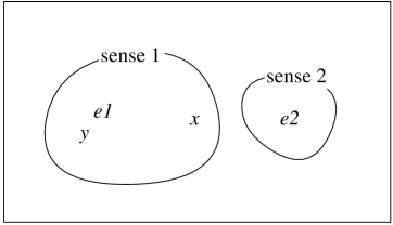
Figure 15: A case where either $x$ or $y$ can be selected in committee-based sampling.

Engelson and Dagan ([Engelson and Dagan, 1996] criticized uncertainty sampling ([Lewis and Gale, 1994], which they call a “single model” approach, as distinct from their “multiple model” approach:

sufficient statistics may yield an accurate 0.51 probability estimate for a class $c$ in a given example, making it certain that $c$ is the appropriate classification. However, the certainty that $c$ is the correct classification is low, since there is a 0.49 chance that $c$ is the wrong class for the example. A single model can be used to estimate only the second type of uncertainty, which does not correlate directly with the utility of additional training. (p.325)

We note that this criticism cannot be applied to our sampling method, despite the fact that our method falls into the category of a single model approach. In our sampling method, given sufficient statistics, the increment of the certainty degree for unsupervised examples, i.e., the training utility of additional supervised examples, becomes small (theoretically, for both example-based and statistics-based systems). Thus, the utility factor can be considered to correlate directly with additional training, for our method.

5 Conclusion

Corpus-based approaches have recently pointed the way to a promising trend in word sense disambiguation. However, these approaches tend to require a considerable overhead for supervision in constructing a large-sized database, additionally resulting in a computational overhead to search the database. To overcome these problems, our method, which is currently applied to an example-based verb sense disambiguation system, selectively samples a smaller-sized subset from a given example set. This method is expected to be applicable to other example-based systems. Applicability for other types of systems needs to be further explored.

The process basically iterates through two phases: (normal) word sense disambiguation and a training phase. During the disambiguation phase, the system is provided with sentences containing a polysemous verb, and searches the database for the most semantically similar example to the input (nearest neighbor resolution). Thereafter, the verb is disambiguated by superimposing the sense of the verb appearing in the supervised example. The similarity between the input and an example, or more precisely the similarity between the case fillers included in them, is computed based on an existing thesaurus. In the training phase, a sample is then selected from the system outputs and provided with the correct interpretation by a human expert. Through these two phases, the system iteratively accumulates supervised examples into the database. The critical issue in this process is to decide which example should be selected as a sample in each iteration. To resolve this problem, we considered the following properties: (a) an example that neighbors more unsupervised examples is more influential for subsequent training, and therefore more informative, and (b) since our verb sense disambiguation is based on nearest neighbor resolution, an example similar to one already existing in the database is redundant. Motivated by these properties, we introduced and formalized the concept of training utility as the criterion for example selection. Our sampling method always gives preference to that example which maximizes training utility.

We reported on the performance of our sampling method by way of experiments in which we compared our method with random sampling, uncertainty sampling ([Lewis and Gale, 1994] and committee-based sampling ([Engelson and Dagan, 1996]. The result of the experiments showed that our method reduced both the overhead for supervision and the overhead for searching the database to a larger degree than any of the above three methods, without degrading the performance of verb sense disambiguation. Through the experiment and discussion, we claim that uncertainty sampling considers property (b) mentioned above, but lacks property (a). We also claim that committee-based sampling differs from our sampling method in terms of its suitability to statistics-based systems as compared to example-based systems.

Acknowledgments

The authors would like to thank Manabu Okumura (JAIST, Japan), Timothy Baldwin (TITECH, Japan), Michael Zock (LIMSI, France), Dan Tufis (Romanian Academy, Romania) and anonymous reviewers for their comments on an earlier version of this paper. This research is partially supported by a Research Fellowship of the Japan Society for the Promotion of Science for Young Scientists.

References

- [Aha, Kibler, and Albert, 1991] Aha, David W., Dennis Kibler, and Marc K. Albert. 1991. Instance-based learning algorithms. Machine Learning, 6(1):37–66.
- [Brown, Pietra, and Pietra, 1991] Brown, Peter F., Stephen A. Della Pietra, and Vincent J. Della Pietra. 1991. Word-sense disambiguation using statistical methods. In Proceedings of the 29th Annual Meeting, pages 264–270, Association for Computational Linguistics.
- [Bruce and Wiebe, 1994] Bruce, Rebecca and Janyce Wiebe. 1994. Word-sense disambiguation using decomposable models. In Proceedings of the 32nd Annual Meeting, pages 139–146, Association for Computational Linguistics.
- [Chapman, 1984] Chapman, Robert L. 1984. Roget’s International Thesaurus (Fourth Edition). Harper and Row.
- [Charniak, 1993] Charniak, Eugene. 1993. Statistical Language Learning. MIT Press.
- [Cohn, Atlas, and Ladner, 1994] Cohn, David, Les Atlas, and Richard Ladner. 1994. Improving generalization with active learning. Machine Learning, 15(2):201–221.
- [Dagan and Itai, 1994] Dagan, Ido and Alon Itai. 1994. Word sense disambiguation using a second language monolingual corpus. Computational Linguistics, 20(4):563–596.
- [Engelson and Dagan, 1996] Engelson, Sean P. and Ido Dagan. 1996. Minimizing manual annotation cost in supervised training from corpora. In Proceedings of the 34th Annual Meeting, pages 319–326, Association for Computational Linguistics.
- [Frakes and Baeza-Yates, 1992] Frakes, William B. and Ricardo Baeza-Yates. 1992. Information Retrieval: Data Structure & Algorithms. PTR Prentice-Hall.
- [Fujii et al., 1996] Fujii, Atsushi, Kentaro Inui, Takenobu Tokunaga, and Hozumi Tanaka. 1996. To what extent does case contribute to verb sense disambiguation? In Proceedings of the 16th International Conference on Computational Linguistics, pages 59–64.
- [Fukumoto and Tsujii, 1994] Fukumoto, Fumiyo and Jun’ichi Tsujii. 1994. Automatic recognition of verbal polysemy. In Proceedings of the 15th International Conference on Computational Linguistics, pages 764–768.
- [Gale, Church, and Yarowsky, 1992] Gale, William, Kenneth Ward Church, and David Yarowsky. 1992. Estimating upper and lower bounds on the performance of word-sense disambiguation programs. In Proceedings of the 30th Annual Meeting, pages 249–256, Association for Computational Linguistics.
- [Gale, Church, and Yarowsky, 1993] Gale, William, Kenneth Ward Church, and David Yarowsky. 1993. A method for disambiguating word senses in a large corpus. Computers and the Humanities, 26:415–439.
- [Guthrie et al., 1991] Guthrie, Joe A., Louise Guthrie, Yorick Wilks, and Homa Aidinejad. 1991. Subject-dependent co-occurrence and word sense disambiguation. In Proceedings of the 29th Annual Meeting, pages 146–152, Association for Computational Linguistics.
- [Hearst, 1991] Hearst, Marti A. 1991. Noun homograph disambiguation using local context in large text corpora. In Proceedings of the 7th Annual Conference of the University of Waterloo Centre for the New OED and Text Research, pages 1–22.
- [Hindle, 1990] Hindle, Donald. 1990. Noun classification from predicate-argument structures. In Proceedings of the 28th Annual Meeting, pages 268–275, Association for Computational Linguistics.
- [Hirst, 1987] Hirst, Graeme. 1987. Semantic Interpretation and the Resolution of Ambiguity. Cambridge University Press.
- [Information-technology Promotion Agency, 1987] Information-technology Promotion Agency. 1987. IPAL Japanese dictionary for computers (basic verbs) (in Japanese).
- [Japan Electronic Dictionary Research Institute, 1995] Japan Electronic Dictionary Research Institute. 1995. EDR electronic dictionary technical guide (in Japanese).
- [Kaji, Kida, and Morimoto, 1992] Kaji, Hiroyuki, Yuuko Kida, and Yasutsugu Morimoto. 1992. Learning translation templates from bilingual text. In Proceedings of the 14th International Conference on Computational Linguistics, pages 672–678.
- [Kameda, 1996] Kameda, Masayuki. 1996. A portable & quick Japanese parser : QJP. In Proceedings of the 16th International Conference on Computational Linguistics, pages 616–621.
- [Karov and Edelman, 1996] Karov, Yael and Shimon Edelman. 1996. Learning similarity-based word sense disambiguation. In Proceedings of the 4th Workshop on Very Large Corpora, pages 42–55.
- [Krovets and Croft, 1992] Krovets, Robert and W. Bruce Croft. 1992. Lexical ambiguity and information retrieval. ACM Transactions on Information Systems, 10(2):115–141.
- [Kurohashi and Nagao, 1994] Kurohashi, Sadao and Makoto Nagao. 1994. A method of case structure analysis for Japanese sentences based on examples in case frame dictionary. IEICE Transactions on Information and Systems, E77-D(2):227–239.
- [Leacock, Towell, and Voorhees, 1993] Leacock, Claudia, Geoffrey Towell, and Ellen Voorhees. 1993. Corpus-based statiscal sense resolution. In Proceedings of ARPA Human Language Technology Workshop, pages 260–265.
- [Lewis and Gale, 1994] Lewis, David D. and William A. Gale. 1994. A sequential algorithm for training text classifiers. In Proceedings of the 17th Annual International ACM SIGIR Conference on Research and Development in Information Retrieval, pages 3–12.
- [Li, Szpakowicz, and Matwin, 1995] Li, Xiaobin, Stan Szpakowicz, and Stan Matwin. 1995. A WordNet-based algorithm for word sense disambiguation. In Proceedings of the 14th International Joint Conference on Artficial Intelligence, pages 1368–1374.
- [Lytinen, 1986] Lytinen, Steven L. 1986. Dynamically combining syntax and semantics in natural language processing. In Proceedings of AAAI-86, pages 574–578.
- [Mainichi Shimbun, 1991-1994] Mainichi Shimbun. 1991-1994. Mainichi shimbun CD-ROM ’91-’94 (in Japanese).
- [Matsumoto et al., 1993] Matsumoto, Yuji, Sadao Kurohashi, Takehito Utsuro, Yutaka Myoki, and Makoto Nagao, 1993. JUMAN Users Manual (in Japanese). Kyoto University and Nara Institute of Science and Technology.
- [Miller et al., 1993] Miller, George A., Richard Beckwith, Christiane Fellbaum, Derek Gross, Katherine Miller, and Randee Tengi. 1993. Five papers on WordNet. Technical Report CLS-Rep-43, Cognitive Science Laboratory, Princeton University.
- [Mooney, 1996] Mooney, Raymond J. 1996. Comparative experiments on disambiguating word senses: An illustration of the role of bias in machine learning. In Proceedings of the Conference on Empirical Methods in Natural Language Processing, pages 82–91.
- [Nagao, 1994] Nagao, Katashi. 1994. A preferential constraint satisfaction technique for natural language analysis. IEICE Transactions on Information and Systems, E77-D(2):161–170.
- [Nagao, 1984] Nagao, Makoto. 1984. A framework of a mechanical translation between Japanese and English by analogy principle. Artificial and Human Intelligence, pages 173–180.
- [Nasukawa, 1993] Nasukawa, Tetsuya. 1993. Discourse constraint in computer manuals. In Proceedings of the 5th Internatinal Conference on Theoretical and Methodological Issues in Machine Translation, pages 183–194.
- [National Language Research Institute, 1964] National Language Research Institute. 1964. Bunruigoihyo (in Japanese). Shuei publisher.
- [Ng, 1997] Ng, Hwee Tou. 1997. Exemplar-based word sense disambiguation: Some recent improvements. In Proceedings of the 2nd Conference on Empirical Methods in Natural Language Processing, pages 208–213.
- [Ng and Lee, 1996] Ng, Hwee Tou and Hian Beng Lee. 1996. Integrating multiple knowledge sources to disambiguate word sense: An exemplar-based approach. In Proceedings of the 34th Annual Meeting, pages 40–47, Association for Computational Linguistics.
- [Niwa and Nitta, 1994] Niwa, Yoshiki and Yoshihiko Nitta. 1994. Co-occurrence vectors from corpora vs. distance vectors from dictionaries. In Proceedings of the 15th International Conference on Computational Linguistics, pages 304–309.
- [Nomiyama, 1993] Nomiyama, Hiroshi. 1993. Machine translation by case generalization (in Japanese). Transactions of Information Processing Society of Japan, 34(5):905–912.
- [Pedersen, Bruce, and Wiebe, 1997] Pedersen, Ted, Rebecca Bruce, and Janyce Wiebe. 1997. Sequential model selection for word sense disambiguation. In Proceedings of the 5th Conference on Applied Natural Language Processing, pages 388–395.
- [Pustejovsky and Boguraev, 1993] Pustejovsky, James and Branimir Boguraev. 1993. Lexical knowledge representation and natural language processing. Artificial Intelligence, 63(1–2):193–223.
- [Real World Computing Partnership, 1995] Real World Computing Partnership. 1995. RWC text database (in Japanese).
- [Resnik, 1993] Resnik, Philip. 1993. Selection and Information: A Class-Based Approach to Lexical Relationships. Ph.D. thesis, University of Pennsylvania.
- [Ribas, 1995] Ribas, Francesc. 1995. On learning more appropriate selectional restrictions. In Proceedings of the 7th Conference of the European Chapter of the Association for Computational Linguistics, pages 112–118.
- [Salton and McGill, 1983] Salton, Gerard and Michael J. McGill. 1983. Introduction to Modern Information Retrieval. McGraw-Hill.
- [Schütze, 1992] Schütze, Hinrich. 1992. Dimensions of meaning. In Proceedings of Supercomputing, pages 787–796.
- [Seung, Opper, and Sompolinsky, 1992] Seung, H. S., M. Opper, and H. Sompolinsky. 1992. Query by committee. In Proceedings of the 5th Annual ACM Workshop on Computational Learning Theory, pages 287–294.
- [Smyth and Keane, 1995] Smyth, Barry and Mark T. Keane. 1995. Remembering to forget: A competence-preserving case deletion policy for case-based reasoning systems. In Proceedings of the 14th International Joint Conference on Artficial Intelligence, pages 377–382.
- [Tokunaga, Iwayama, and Tanaka, 1995] Tokunaga, Takenobu, Makoto Iwayama, and Hozumi Tanaka. 1995. Automatic thesaurus construction based on grammatical relations. In Proceedings of the 14th International Joint Conference on Artficial Intelligence, pages 1308–1313.
- [Uramoto, 1994a] Uramoto, Naohiko. 1994a. A best-match algorithm for broad-coverage example-based disambiguation. In Proceedings of the 15th International Conference on Computational Linguistics, pages 717–721.
- [Uramoto, 1994b] Uramoto, Naohiko. 1994b. Example-based word-sense disambiguation. IEICE Transactions on Information and Systems, E77-D(2):240–246.
- [Utsuro, 1996] Utsuro, Takehito. 1996. Sense classification of verbal polysemy based-on bilingual class/class association. In Proceedings of the 16th International Conference on Computational Linguistics, pages 968–973.
- [Utsuro et al., 1994] Utsuro, Takehito, Kiyotaka Uchimoto, Mitsutaka Matsumoto, and Makoto Nagao. 1994. Thesaurus-based efficient example retrieval by generating retrieval queries from similarities. In Proceedings of the 15th International Conference on Computational Linguistics, pages 1044–1048.
- [Voorhees, 1993] Voorhees, Ellen M. 1993. Using WordNet to disambiguate word senses for text retrieval. In Proceedings of the 16th Annual International ACM SIGIR Conference on Research and Development in Information Retrieval, pages 171–180.
- [Yarowsky, 1992] Yarowsky, David. 1992. Word-sense disambiguation using statistical models of Roget’s categories trained on large corpora. In Proceedings of the 14th International Conference on Computational Linguistics, pages 454–460.
- [Yarowsky, 1995] Yarowsky, David. 1995. Unsupervised word sense disambiguation rivaling supervised methods. In Proceedings of the 33rd Annual Meeting, pages 189–196, Association for Computational Linguistics.
- [Zernik, 1989] Zernik, Uri. 1989. Lexicon acquisition: Learning from corpus by capitalizing on lexical categories. In Proceedings of the 11th International Joint Conference on Artficial Intelligence, pages 1556–1562.