A Differential Invariant for Zooming

Abstract

This paper presents an invariant under scaling and linear brightness change. The invariant is based on differentials and therefore is a local feature. Rotationally invariant 2-d differential Gaussian operators up to third order are proposed for the implementation of the invariant. The performance is analyzed by simulating a camera zoom-out.

1 Introduction

In image retrieval systems, efficiency depends prominently on identifying features that are invariant under the transformations that may occur, since such invariants reduce the search space. Such transformations typically include translation, rotation, and scaling, as well as linear brightness changes. Ideally, we would like to consistently identify key points whose features are invariant under those transformations.

Geometrical invariants have been known for a long time, and they have been applied more recently to vision tasks [7, 9]. Differential invariants are of particular interest since they are local features and therefore more robust in the face of occlusion. Building on a suggestion by Schmid and Mohr [8], we propose an invariant with respect to the four aforementioned transformations, based on derivatives of Gaussians.

In the following, we restrict ourselves to 2-d objects, i.e. we assume that the objects of interest are not rotated outside the image plane, and that they are without significant depth so that the whole object is in focus simultaneously. The lighting geometry also remains constant. In other words, we allow only translation and rotation in the image plane, scaling that reduces the size of an object (zoom-out), and brightness changes by a constant factor. The zooming can be achieved by either changing the distance between object and camera or by changing the focal length.

2 The Invariant

2.1 The 1-d case

Schmid and Mohr [8] have presented the following invariant under scaling. Let $f(x)=g(u(x))=g(\alpha x)$, i.e. g(u) is derived from f(x) by a change of variable with scaling factor $\alpha$. Then $f(x)=g(u),f^{\prime}(x)=\alpha g^{\prime}(u),f^{\prime\prime}(x)=\alpha^{2}g^{\prime\prime}(u)$, and thus $\Theta_{12}=f^{\prime}(x)^{2}/f^{\prime\prime}(x)$ is an invariant to scale change. This invariant generalizes to

$$\Theta_{SM}(f(x))=\frac{[f^{(n)}(x)]^{k/n}}{f^{(k)}(x)}$$ (1)

where $k,n\in\mathbb{N}$ denote the order of the derivatives.

$\Theta_{SM}$ is not invariant under linear brightness change. But such an invariance is desirable because it would ensure that properties that can be expressed in terms of the level curves of the signal are invariant [5]. A straightforward modification of $\Theta_{12}$ gives us the extended invariance: Let $f(x)=k\,g(u)=k\,g(\alpha x)$ where $k$ is the brightness factor. Then $f^{\prime}(x)=k\alpha\,g^{\prime}(u),f^{\prime\prime}(x)$ = $k\alpha^{2}\,g^{\prime\prime}(u),f^{\prime\prime\prime}(x)=k\alpha^{3}\,g^{\prime\prime\prime}(u)$. It can be seen that

$$\Theta_{123}(f(x))=\frac{f^{\prime}(x)\ f^{\prime\prime\prime}(x)}{f^{\prime\prime}(x)^{2}}=\frac{k\alpha\,g^{\prime}(u)\ k\alpha^{3}\,g^{\prime\prime\prime}(u)}{(k\alpha^{2}\,g^{\prime\prime}(u))^{2}}$$

has the desired invariance since both $\alpha$ and $k$ cancel out. $\Theta_{123}$ can be generalized to $\Theta_{g3}=f^{(k)}(x)\ f^{(k+2)}(x)/$ $f^{(k+1)}(x)^{2}$ where $k\in\mathbb{N}$, but $k>1$ is of little interest in computer vision.

An obvious shortcoming of $\Theta_{123}$, as well as of the other scale invariants discussed so far, is that they are undefined where the denominator is zero. Therefore, we modify $\Theta_{123}$ to be continuous everywhere:

0 if c1

$$\Theta_{m123}(f(x))=$$ if c2

else

(2)

where c1 is the condition $f^{\prime\prime}(x)=0\wedge f^{\prime}(x)f^{\prime\prime\prime}(x)=0$, and c2 specifies $|f^{\prime}(x)f^{\prime\prime\prime}(x)|<|f^{\prime\prime}(x)^{2}|$. Note that this definition results in $-1\leq\Theta_{m123}\leq 1$.

2.2 The 2-d case

If we are to apply eq. 2 to images, we have to generalize the formula to two dimensions. Also, images are given typically in the form of sampled intensity values rather than in the form of closed formulas where derivatives can be computed analytically. One way to combine filtering with the computation of derivatives can be provided by using Gaussian derivatives [1, 5, 8]. Let $I_{1}(x,y)$ and $I_{2}(u,v)=I_{2}(\alpha x,\alpha y)$ be two images related by a scaling factor $\alpha$. Then, according to Schmid and Mohr [8],

$$\int_{-\infty}^{\infty}I_{1}(x,y)\circledast G_{i_{1}\dots i_{n}}(x,y;\sigma)\,dx\,dy$$ =

    

(3)

where the $G_{i_{1}\dots i_{n}}$ are partial derivatives of the 2-d Gaussian.

Rotational invariance is a highly desirable property in most image retrieval tasks. While derivatives are translation invariant, the partial derivatives in eq. 3 are not rotationally invariant. However, there are some well-known rotationally invariant differential operators. Recall that the 2-d zero mean Gaussian is defined as

$$G(x,y;\sigma)=\frac{1}{2\pi\,\sigma^{2}}\ e^{-\frac{x^{2}+y^{2}}{2\sigma^{2}}}$$ (4)

Then the gradient magnitude

$$|\mathrm{grad}\ G(x,y;\sigma)|=\sqrt{G_{x}^{2}+G_{y}^{2}}=\sqrt{x^{2}+y^{2}}/\sigma^{2}\ G$$ (5)

is a first order differential operator with the desired property. Horn [3] gives the following second order operators:

$$\mathrm{LoG}(x,y;\sigma)$$ =

=

(6)

$$\mathrm{QV}(x,y;\sigma)$$ =

=

(7)

where LoG is the Laplacian of Gaussian. QV stands for Quadratic Variation where we have taken the square root in order to avoid high powers. Schmid and Mohr also suggest what they call $\nu[2]$:

$$\nu[2](x,y;\sigma)$$ =

    =

(8)

Analogous to QV, we define a third order differential operator which we call Cubic Variation to be

$$\mathrm{CV}(x,y;\sigma)$$ =

    =

(9)

By contrast, Schmid and Mohr use

$$\nu[6](x,y;\sigma)$$ =

    + 

=

(10)

and

$$\nu[8](x,y;\sigma)$$ =

    + 

=

(11)

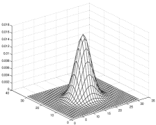
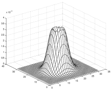
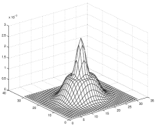
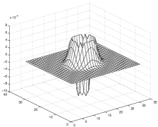
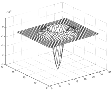
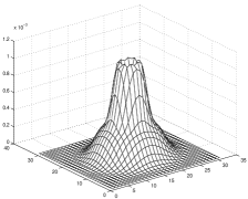
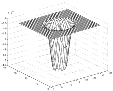
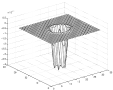
Figure 2: Rotationally invariant 2-d differential operators, $\sigma=3.0$:  (a) Gaussian  (b) Gradient  (c) Quadratic Variation  (d) $\nu[2]$  (e) Laplacian of Gaussian  (f) Cubic Variation  (g) $-\sqrt{\nu[6]}$  (h) $\nu[8]$.

These operators are shown in fig. 2 for $\sigma=3$. Given this choice of operators, the criteria on which we select the operators are as follows:

• The operator must fulfill eq. 3, i.e. scaling by $\alpha$ (of both $x$ and $y$ simultaneously) should return a factor of $\alpha^{n}$, where $n$ is the order of the operator, so that eq. 2 is indeed a scale invariant.

• The operators used to compute $\Theta_{m123}$ should differ in shape as much as possible from each other in order to deliver more discriminative results.

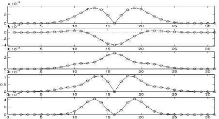
Figure 3: Cross sections through differential operators, $\sigma=3.0$:  (a) Gradient  (b) Laplacian of Gaussian  (c) Quadratic Variation  (d) Cubic Variation  (e) $\sqrt{\nu[6]}$. The circles mark the filter coefficients.

With respect to the first criterion, the gradient returns a factor $\alpha^{1}$, as required for a first order differential operator, and the LoG and QV return a factor of $\alpha^{2}$, but $\nu[2]$ returns $\alpha^{4}$. This cannot be remedied by taking the square root since $\nu[2]$ is negative at some points. As for the third order operators, CV returns $\alpha^{3}$, while $\nu[6]$ and $\nu[8]$ return $\alpha^{6}$. We can take the square root of $\nu[6]$ but not of $\nu[8]$. Where the second criterion is concerned, the LoG is preferable to QV since the LoG has both positive and negative coefficients, which makes it unique compared to all other operators. It is not obvious whether CV or $\sqrt{\nu[6]}$ has more discriminatory power, the difference between them seems negligible. $\sqrt{\nu[6]}$ has a slightly more compact support, but the coefficients are an order of magnitude smaller than those of CV and the other operators. Fig. 3 shows cross sections through the center of some of the operators in fig. 2. In our experiments, we used the Gradient, LoG, and CV as the differential operators to compute $\Theta_{m123}$ according to eq. 2. Since Gradient and CV are always positive or zero, we have $0\leq\Theta_{m123}\leq 1$.

Note that eqs. 5 to 11 suggest two ways of implementation. Either, kernels representing the partial derivatives of the Gaussian can be used, and the operators are assembled from those kernels according to the left hand sides of the equations, or a characteristic filter is designed in each case according to the right hand sides of the equations.

3 Simulation

The infinite integrals in eq. 3 can only be approximated by sampled, finite signals and filters. Furthermore, in cameras, where the number of pixels is constant, a world object is mapped into fewer pixels as the camera zooms out, leading to increasing spatial integration over the object and ultimately to aliasing. This means that the computation of $\Theta_{m123}$ necessarily has an error. Equation 3 suggests a way to analyze the accuracy of $\Theta_{m123}$ by simulating the zoom-out process. The left hand side can be thought of as a scaling by filtering (SF) process while the right hand side could be called scaling by optical zooming (SO) where we deal with a scaled, i.e. reduced image and an appropriately adjusted Gaussian operator. Here, scaling by optical zooming serves to simulate the imaging process as the camera moves away from an object. The two processes are schematically depicted in fig. 1.

The input to the simulation are 8-bit images taken by a real camera. The scaling factor $\alpha$ is a free parameter, but it is chosen such that the downsampling maps an integer number of pixels into integers. Both SF and SO start off with a lowpass filtering step. This prefiltering, implemented by a Gaussian with $\sigma=\alpha$, improves the robustness of the computations significantly as derivatives are sensitive to noise. Also, lowpass filtering reduces aliasing at the subsequent downsampling step.

In SO, if the image function had a known analytical form, we could do the scaling by replacing the spatial variables $x$ and $y$ by $\alpha x$ and $\alpha y$. But images are typically given as intensity matrices. Therefore, the downscaling is done by interpolation, using cubic splines. We then apply the differential operators (Gradient, LoG, CV) with the appropriate value of $\alpha\sigma$ to the image and compute the invariant $\Theta_{m123}^{SO}$. By contrast, in SF, the operators are applied to the original size image. The invariants are computed and then downscaled, using again cubic spline interpolation, to the same size as the image coming out of the SO process, so that $\Theta_{m123}^{SO}$ and $\Theta_{m123}^{SF}$ can be compared directly at each pixel.

Figure 1: (left) scaling by filtering process vs. (right) scaling by simulated optical zooming.

4 Experiments

Fig. 4 demonstrates the simulation process on a real image. The original image, 256$\times$256, in the top row, is downscaled to 100$\times$100, i.e. by a factor $\alpha=2.56$. The second and third row show $\Theta_{m123}$ as the results of SF and SO, respectively, at all pixel locations. Fig. 5 shows the absolute difference between $\Theta_{m123}^{SF}$ and $\Theta_{m123}^{SO}$, where the four boundary rows and columns have been set to zero in order to mask the boundary effects. Note that the difference is roughly a factor 100 smaller than the values of $\Theta_{m123}^{SO}$ or $\Theta_{m123}^{SF}$.

In order to quantify the error, we have varied $\alpha$ from 1 to 2.56, sampled such that the downscaled image has an integer pixel size, and computed the global absolute differences

$$\Delta_{\Theta_{m123}}(\alpha)=\max_{i,j}\,(|\Theta_{m123}^{SO}-\Theta_{m123}^{SF}|)$$ (12)

where $i,j$ range over all non-boundary pixels of the respective image, as well as the global relative error, in percent:

$$\epsilon_{gr}(\alpha)=100\,\frac{\Delta_{\Theta_{m123}}}{\max_{i,j}\,(|\Theta_{m123}^{SO}|)}$$ (13)

The graphs of these measures are shown in fig. 7. We see that the global relative error is less than 1.3% even as $\alpha$ becomes as large as 2.56. For the set of images we worked with, we have observed $0.5\%<\max(\epsilon_{gr})<2\%$ for $\alpha<3$. We also noted that without prefiltering $\epsilon_{gr}$ can become as large as 10%.

Fig. 6 shows the relative error per pixel in percent, i.e. $100\,\Delta_{\Theta_{m123}}(i,j)\,/\,|\Theta_{m123}^{SO}(i,j)|$, but only for those pixels $(i,j)$ where $\Theta_{m123}^{SO}(i,j)$ is larger than the average value of $\Theta_{m123}^{SO}$. We find that error to be less than 3.5% anywhere in the given example.

5 Outlook

In the context of image retrieval, there remain some major issues to be addressed. First, the performance of the proposed invariant has to be analyzed on sequences of images taken at increasing object-camera distance, i.e. the simulation of the zoom-out process has to be replaced with a true camera zoom-out. Intrinsic limitations of the image formation process by CCD cameras [2] can be expected to somewhat decrease the accuracy of the invariant.

Second, a scheme for keypoint extraction must be devised. For efficiency reasons, matching will be done on those keypoints only. Ideally, the keypoints should be reliably identifiable, irrespective of scale.

Third, the proposed invariant must be combined with a scale selection scheme. Note that in the simulation above, we knew a priori the right values for $\alpha$ and therefore for $\alpha\sigma$ and the corresponding filter size. But such is not the case in general object retrieval tasks. Selecting stable scales is an active research area [5, 6].

6 Acknowledgements

The author would like to thank Bob Woodham and David Lowe for their valuable feedback.

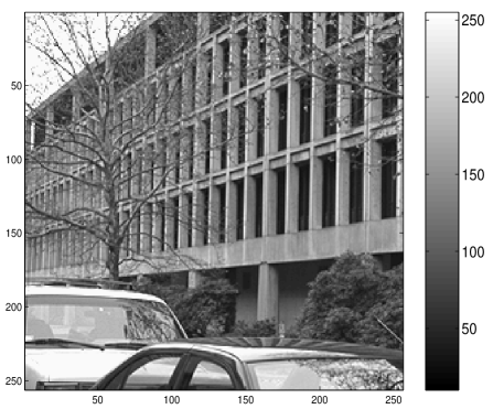
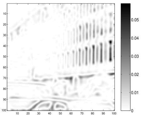
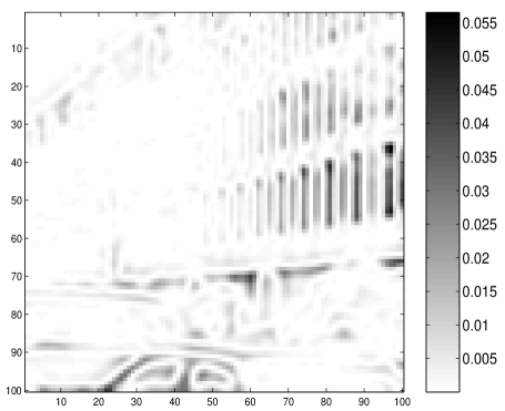
Figure 4: (a) Original 256x256 image  (b) $\Theta_{m123}^{SF}$ for $\alpha=2.56$  (c) $\Theta_{m123}^{SO}$ for $\alpha=2.56$.

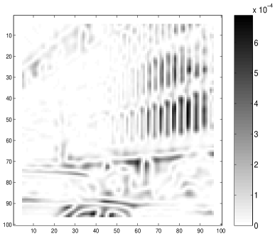
Figure 5: Absolute difference $|\Theta_{m123}^{SO}-\Theta_{m123}^{SF}|$. Note the smaller scale ($10^{-4}$) of the error compared to fig. 4.

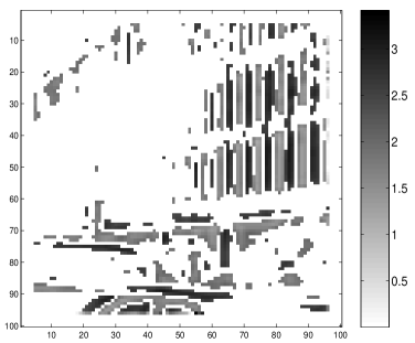
Figure 6: Relative Errors at above-average values of $\Theta_{m123}^{SO}$ for $\alpha=2.56$, in percent.

Figure 7: (a) $\Delta_{\Theta_{m123}}(\alpha)$,  (b) $\max_{i,j}\,(|\Theta_{m123}^{SO}|)(\alpha)$,  (c) $\epsilon_{gr}(\alpha)$, over image size in pixels;  $1\leq\alpha\leq 2.56$.

References

- [1] B. ter Haar Romeny, “Geometry-Driven Diffusion in Computer Vision”, Kluwer 1994.
- [2] G. Holst, “Sampling, Aliasing, and Data Fidelity”, JCD Publishing & SPIE Press, 1998.
- [3] B. Horn, “Robot Vision”, MIT Press, 1986.
- [4] A. Jain, “Fundamentals of Digital Image Processing”, Prentice-Hall, 1989.
- [5] T. Lindeberg, “Scale-Space Theory: A Basic Tool for Analysing Structures at Different Scales”, J. of Applied Statistics, Vol.21, No.2, pp.223-261, 1994.
- [6] D. Lowe, “Object Recognition from Local Scale-Invariant Features”, ICCV, Kerkyra 1999.
- [7] J. Mundy, A. Zisserman, “Geometric Invariance in Computer Vision”, MIT Press, Cambridge 1992.
- [8] C. Schmid, R. Mohr, “Local grayvalue invariants for Image Retrieval”, IEEE Trans. PAMI, Vol.19, No.5, pp.530-535, May 1997.
- [9] I. Weiss, “Geometric Invariants and Object Recognition”, Int.Journal of Computer Vision, Vol.10, No.3, pp.207-231, 1993.