Quadrilateral Meshing by Circle Packing

Abstract

We use circle-packing methods to generate quadrilateral meshes for polygonal domains, with guaranteed bounds both on the quality and the number of elements. We show that these methods can generate meshes of several types: (1) the elements form the cells of a Voronoï diagram, (2) all elements have two opposite $90^{\circ}$ angles, (3) all elements are kites, or (4) all angles are at most $120^{\circ}$. In each case the total number of elements is $O(n)$, where $n$ is the number of input vertices.

1 Introduction

We investigate here problems of unstructured quadrilateral mesh generation for polygonal domains, with two conflicting requirements. First, we require there to be few quadrilaterals, linear in the number of input vertices; this is appropriate for methods in which high order basis functions are used, or in multiblock grid generation in which each quadrilateral is to be further subdivided into a structured mesh. Second, we require some guarantees on the quality of the mesh: either the elements themselves should have shapes restricted to certain classes of quadrilaterals, or the mesh should satisfy some more global quality requirements.

Computing a linear-size quadrilateralization, without regard for quality, is quite easy. One can find quadrilateral meshes with few elements, for instance, by triangulating the domain and subdividing each triangle into three quadrilaterals[15]. For convex domains, it is possible to exactly minimize the number of elements[13]. However these methods may produce very poor quality meshes. High-quality quadrilateralization, without rigorous bounds on the number of elements, is an area of active practical interest. Techniques such as paving[7] can generate high-quality meshes for typical inputs; however these meshes may have many more than $O(n)$ elements. Indeed, if the requirements on element quality include a constant bound on aspect ratio, then meshing a rectangle of aspect ratio $A$ will require $\Omega(A)$ quadrilaterals, even though in this case $n=4$.

We provide a first investigation into the problem of finding a suitable tradeoff between those two requirements: for which measures of mesh quality is it possible to find guaranteed-quality meshes with guaranteed linear complexity? The results—and indeed the algorithms—of this paper are analogous to the problem of nonobtuse triangulation[2, 4, 6]. Interestingly, for quadrilaterals there seem to be several analogues of nonobtuseness.

Our algorithms are based on circle packing, a powerful geometric technique useful in a variety of contexts. Specifically, we build on a circle-packing method due to Bern, Mitchell, and Ruppert[6]. In this method, before constructing a mesh, one fills the domain with circles, packed closely together so that the gaps between them are surrounded by three or four tangent circles. (Circle packings with only three-sided gaps form a sort of discrete analogue to conformal mappings[18]. However for most domains some four-sided gaps are necessary, and in some of our algorithms four-sided gaps are actually helpful since they lead to degree-four mesh vertices.) One then uses these circles as a framework to construct the mesh, by placing mesh vertices at circle centers, points of tangency, and within each gap. Earlier work by Shimada and Gossard[17] also uses approximate circle packings and sphere packings to construct triangular meshes of 2-d domains and 3-d surfaces. Other authors have introduced related circle packing ideas into meshing via conforming Delaunay triangulation[14], conformal mapping[8, 16], and decimation[12, 11]. Circle packing ideas closely related to the algorithms in this paper have also been applied in origami design[10, 3].

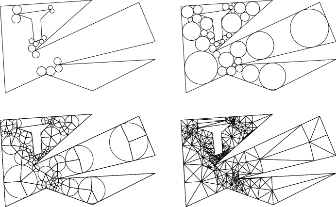
Figure 1: Nonobtuse triangulation steps: (a) protect reflex vertices and connect holes; (b) pack polygon with circles; (c) connect circle centers; (d) triangulate remaining polygonal regions.

We use circle packing to develop four new quadrilateral meshing methods. First, in Section 3, we show that the Voronoï diagram of the points of tangency of a suitable circle packing forms a quadrilateral mesh. Although the individual elements in this mesh may not have good quality, the Voronoï structure of the mesh may prove useful in some applications such as finite volume methods. Second, in Section 4, we overlay this Voronoï mesh with its dual Delaunay triangulation; this overlay subdivides each Voronoï cell into quadrilaterals having two opposite right angles. Note that any such quadrilateral must have all four of its vertices on a common circle. Third, in Section 5, we show that a small change to the method of Bern et al. (basically, omitting some edges), produces a mesh of kites (quadrilaterals having two adjacent pairs of equal-length sides). The resulting mesh optimizes the cross ratio of the elements (a measure of the aspect ratio of the rectangles into which each element may be conformally mapped): any kite can be conformally mapped onto a square. Finally, in Section 6, we subdivide these kites into smaller quadrilaterals, producing a mesh in which each quadrilateral has maximum angle at most $120^{\circ}$. This is optimal: there exist domains for which no mesh has angles better than $120^{\circ}$.

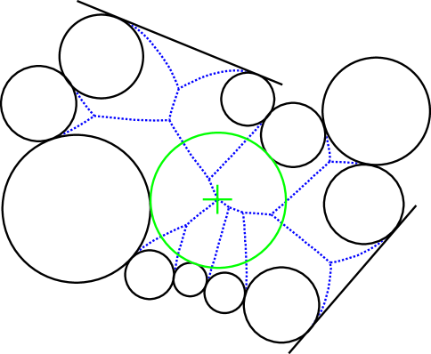
Figure 2: Placement of a new circle centered on a Voronoï vertex partitions a region bounded by circular arcs into several simpler regions.

2 Circle Packing

Let us first review the nonobtuse triangulation method of Bern et al.[6]. This algorithm is given an $n$-vertex polygonal region (possibly with holes), and outputs a triangulation with $O(n)$ new Steiner points in which no triangle has an obtuse angle. In outline, it performs the following steps:

1. Protect reflex vertices of the polygon by placing circles tangent to the boundary of the polygon on either side of them, small enough that they do not intersect each other or other features of the polygon (Figure 1(a)).

2. Connect holes of the polygon by placing nonoverlapping circles, tangent to edges of the polygon or to previously placed circles, so that the domain outside the circles forms one or more simply connected regions with circular-arc sides.

3. Simplify each region by packing it with further circles until each remaining region has three or four circular-arc or straight-line sides (Figure 1(b)).

4. Partition the polygon into 3- and 4-sided polygonal regions by connecting the centers of tangent circles (Figure 1(c)).

5. Triangulate each region with nonobtuse triangles (Figure 1(d)).

Our quadrilateralization algorithms will be based on the same general outline, and in several cases the quadrilaterals we form can be viewed as combinations of several of the triangles formed by this algorithm.

Steps 1, 4, and 5 are straightforward to implement. Eppstein[9] showed that step 2 could be implemented efficiently, in time $O(n\mathop{\rm log}n)$, as independently did Mike Goodrich and Roberto Tamassia, and Warren Smith (unpublished). We now describe in some more detail step 3, simplification of regions, as we will need to modify this step in some of our algorithms.

Lemma 1 (Bern et al.[6])

Any simply connected region of the plane bounded by $n$ circular arcs and straight line segments, meeting at points of tangency, can be packed with $O(n)$ additional circles in $O(n\mathop{\rm log}n)$ time, such that the remaining regions between circles are bounded by at most four tangent circular arcs.

Proof: Compute the Voronoï diagram of the circles within this region; that is, a partition of the region into cells, each of which contains points closer to one of the circles than to any other circle (Figure 2). Because the region is simply connected, the cell boundaries of this diagram form a tree. We choose a vertex $v$ of this tree such that each of the subtrees rooted at $v$ has at most half the leaves of the overall tree, and draw a circle centered at $v$ and tangent to the circles having Voronoï cells incident at $v$. This splits the region into simpler regions. We continue recursively within these regions, stopping when we reach regions bounded by only four arcs (in which no further simplification is possible). Adding each new circle to the Voronoï diagram can be done in time linear in the number of arcs bounding the region, so the total time to subdivide all regions is $O(n\mathop{\rm log}n)$.

We call the region between circles of this packing a gap. We now state without proof two technical results of Bern et al. about these gaps.

Lemma 2 (Bern et al.[6])

The points of tangency on the boundary of a gap are cocircular.

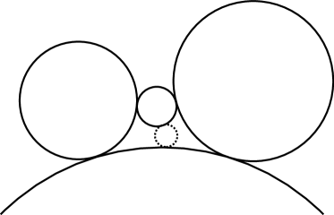
Figure 3: Bad four-sided gap split into two good gaps.

A three-sided gap is one bounded by three circular arcs. A good four-sided gap is a gap bounded by four arcs, such that the circumcenter of its points of tangency is contained within the convex hull of those points. A bad four-sided gap is any other four-arc gap.

Lemma 3 (Bern et al.[6])

Any bad four-sided gap can be split into two good four-sided gaps by the addition of a circle tangent to two of the bad four-sided gap’s circles. (Figure 3.)

In some cases two opposite circles bounding one of the new gaps created by Lemma 3 may overlap, but this poses no problem for the rest of the algorithm.

3 Voronoï Quadrilateralization

Figure 4: Voronoï quadrilateralization of a polygon.

We begin with the quadrilateralization procedure most likely to be useful in practice, due to its low output complexity and lack of complicated special cases.

The geodesic Voronoï diagram of a set of point sites in a polygonal domain is a partition of the domain into cells, in each of which the geodesic distance (distance along paths within the domain) is closest to one of the given sites. We now describe a method of finding a point set for which the geodesic Voronoï diagram forms a quadrilateral mesh. One potential application of this type of mesh would be in the finite volume method, as the dual of this Voronoï mesh could be used to define control volumes for that method (see e.g. Miller et al.[12]). The angle between each primal and dual edge pair would be $90^{\circ}$, causing some terms in the finite volume method to cancel and therefore saving some multiplications[2, 5]. Our mesh will also have the possibly useful property that all Voronoï edges will cross their duals.

We modify the initial circle packing of Bern et al.[6], as follows. We start by protecting vertices, as before; but in this case that protection consists of a circle centered at each domain vertex. Then, as before we fill the remainder of the domain by tangent circles; however we do not attempt to create tangencies with the domain boundary; instead the circle packing should meet the boundary at circles with their centers on the boundary. Further, no tangent point between two circles should lie on the domain boundary, although circles centered on the boundary may meet in the domain interior. (Some circles may cross or be tangent to the boundary, however we ignore these incidences, instead treating these circles as part of three-sided gaps.) It is not hard to modify the previous circle packing algorithms to meet these conditions. The result will be a packing with, again, three-sided and four-sided gaps. However, the gaps involving boundary edges are all four-sided and have right-angled corners rather than points of tangency on those edges.

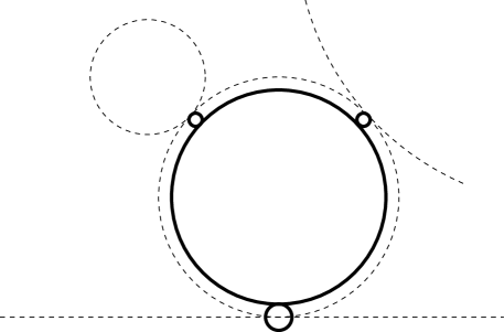
Figure 5: Replacement of disk tangent to boundary by multiple disks centered on boundary.

Theorem 1

In $O(n\mathop{\rm log}n)$ time we can find a circle packing as above, such that the geodesic Voronoï diagram of the points of tangencies of the circles forms a quadrilateral mesh.

Proof: The vertex protection step can be performed in $O(n)$ time using circles with radius half the minimum distance between vertices. (This minimum distance is an edge of the Delaunay triangulation and can be found in $O(n\mathop{\rm log}n)$ time.) Next we find a set of $O(n)$ circles to add to our packing, so that any remaining gaps are simply connected[9]. If in this step we ever add a circle $c$ tangent to the boundary, we replace it by a set of circles: a circle with radius $\epsilon$ centered on the boundary at the point of tangency, circles with radius $\epsilon/2$ tangent to $c$ at each of its other points of tangency, and one circle concentric to $c$ with radius reduced by $\epsilon$; this replacement is depicted in Figure 5.

Finally, as in the algorithm of Bern et al.[6] we repeatedly find the Voronoï diagram of the circles bounding any remaining gap and place a circle on a Voronoï vertex so as to divide the gap into two smaller parts of roughly equal complexity. However, in order to avoid placing circles tangent to the boundary in this step, we change their method by using only the circles around a gap as Voronoï sites, omitting any diagram edges that may bound the gap. Our Voronoi diagram’s edges (together with any boundary edges of the gap) form a tree, so we can find a vertex which splits the tree’s leaves roughly evenly. Placing a circle at that vertex produces two simpler gaps and does not cause essential tangencies with the domain boundary. Unlike Bern et al.[6], we do not bother eliminating bad four-sided gaps.

We form a mesh by connecting each center of a circle in the packing to the circumcenters of adjacent gaps (Figure 4). In the four-sided gaps along the domain boundary, we place an additional edge from the boundary to the center of the opposite circle, bisecting the chord between the tangencies with the two other circles. These edges form a quadrilateral mesh since each face surrounds a point of tangency, and each point of tangency is surrounded by the vertices from two circles and two gaps. Each mesh element is the Voronoi cell of the point of tangency it contains; its boundary is composed of perpendicular bisectors of dual Delaunay edges. Each dual Delaunay edge has a circumscribing circle from the circle packing as witness to the empty-circle property of Delaunay graphs.

Curiously, this mesh is not only a certain type of generalized Voronoï diagram; it is also another type of generalized Delaunay triangulation! The power of a circle with respect to a point in the plane is the squared radius of the circle minus the squared distance of the point to the circle’s center. The power diagram of a set of (not necessarily disjoint) circles is a partition of the plane into cells, each consisting of the points for which the power of some particular circle is greatest. Like the usual kind of Voronoï diagram, the power diagram has convex cells, since the separator between any two circles’ cells is a line (if the two circles overlap, their separator is the line through their two intersection points). We can restrict the power diagram to a polygonal domain by defining the power only for points visible to the center of the given circle.

From the construction above, define a family $F$ of circles by including the original packing and a “dual” collection of circles through the tangencies surrounding each gap, centered at the gap’s site. As we now show, the power diagram of this family (depicted in Figure 6) is the planar dual to our mesh.

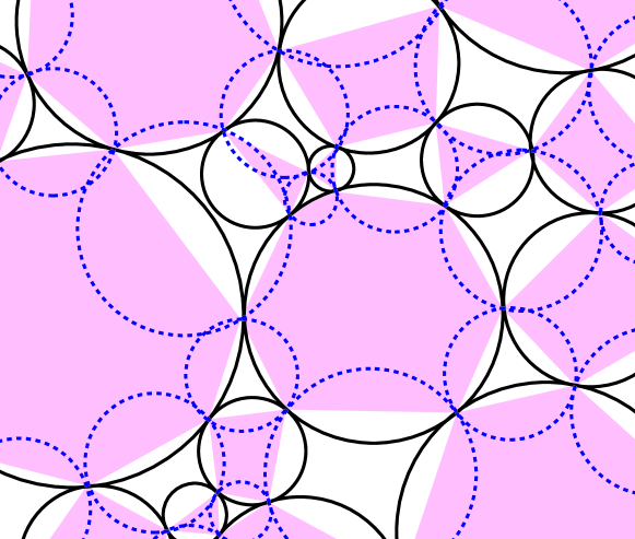
Figure 6: Circle packing (solid circles), circumcircles of gaps (dashed circles), and power diagram (shaded and unshaded polygons).

Theorem 2

The quadrilateral mesh defined above includes an edge between two points if and only if the corresponding circles’ cells share an edge in the power diagram of $F$.

Proof: $F$ has one circle centered at each vertex; the two circles corresponding to the endpoints of an edge overlap in a lune. The lune’s two corners are points of tangency in the original circle packing (or, if the edge is on the domain boundary, the corners are one such point of tangency and its reflection) and are contained in the two quadrilaterals on either side of the edge. These corners have power zero with respect to the two circles, and are not interior to any other circles; therefore they have those two circles (and possibly some others) as nearest power neighbors. Since power diagram cells are convex, those two circles must continue to be the nearest neighbors to each point along the center line of the lune; in other words this center line lies along an edge in the power diagram corresponding to the given mesh edge.

Conversely, we must show that every power diagram adjacency corresponds to a mesh edge. But the power diagram boundaries described above form a convex polygon completely containing the center of the cell’s circle; therefore there can be no other adjacencies than the ones we have already found, which correspond to mesh edges.

Since quadrilaterals in this mesh typically correspond to eight triangles in the nonobtuse triangulation algorithm of Bern et al., the constant factors in the $O(n)$ bound above should be quite small in practice. Bern et al.[6] observed that their method typically generated between $20n$ and $30n$ triangles, so we should expect between $3n$ and $4n$ quadrilaterals in our mesh.

4 Opposite Right Angles

As we now show, the Voronoï triangulation above can be used to find another quadrilateral mesh, in which each quadrilateral has two opposite right angles. Such a quadrilateral must be cyclic (having all four vertices on a common circle); further, the circumcenter bisects the diagonal connecting the two remaining vertices.

Our algorithm works by overlaying the power diagram defined above onto the quadrilaterals of Theorem 1, resulting in their subdivision into smaller quadrilaterals. In order to perform this subdivision, we may need to place a few additional circles into our packing. On the boundary of the domain, the gaps between circles will be formed by chains of three tangent circles, the two ends of which are circles centered on the domain boundary. The center circle in this chain is allowed to cross the boundary; we ignore this crossing. Reflecting such a chain across the domain boundary edge produces a four-sided gap partially outside the domain; like Bern et al.[6] we say that this gap is good or bad if the convex hull of its points of tangency contains or doesn’t contain their circumcenter respectively. The algorithm of this section requires these gaps to be good. As in the method of Bern et al.[6], any bad four-sided gap can be subdivided into two good four-sided gaps by the addition of another circle which by symmetry can be placed with its center on the domain boundary.

Theorem 3

In $O(n\mathop{\rm log}n)$ time we can partition any polygon into a mesh of $O(n)$ quadrilaterals, each having two opposite right angles.

Proof: We form the Voronoï quadrilateralization of Theorem 1, and subdivide each quadrilateral $Q$ into four smaller quadrilaterals by dropping perpendiculars from the Voronoï site contained in $Q$ to each of $Q$’s four sides. On edges where two cells of the Voronoï quadrilateralization meet, the two perpendiculars end at a common vertex because they are the two halves of a chord connecting two tangent points on the same circle. For the same reason, each perpendicular meets the edge to which it is perpendicular without crossing any other cell boundaries first.

The same procedure of dropping perpendiculars will work whenever we have a Voronoï diagram in which the site generating each cell can be connected by a perpendicular to each cell edge. Therefore, some heuristic simplification can be applied to the mesh above, reducing its complexity further: after forming the Voronoï quadrilateralization of Theorem 1, remove sites one by one from the set of generators as long as this condition is met.

5 Kites

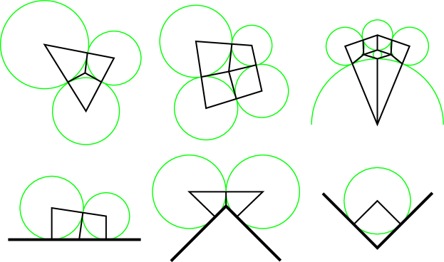
Figure 7: Cases for decomposition into kites: (a) three tangent circles; (b) four tangent circles forming good four-sided gap; (c) bad four-sided gap subdivided into two good four-sided gaps; (d) two tangent circles on boundary; (e) reflex vertex; (f) convex vertex.

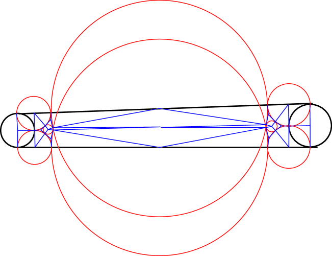
Figure 8: Kite decomposition of four-sided gap with two sides on domain boundary.

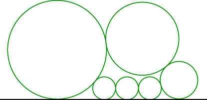
Figure 9: Kite decomposition of four-sided gap with one side on domain boundary: add small circles along boundary edge making three-sided gaps.

The next type of quadrilateralization we describe is one in which all quadrilaterals are kites (convex quadrilaterals with an axis of symmetry along one diagonal). Although kites may have bad angles (very close to $0^{\circ}$ or $180^{\circ}$), they have some other nice theoretical properties. In particular, the cross ratio of a kite is always one.

The cross ratio of a quadrilateral with consecutive side lengths $a$, $b$, $c$, and $d$ is the ratio $ac:bd$. Since this ratio is invariant under conformal mappings, a conformal mapping from the quadrilateral to a rectangle (taking vertices to vertices) can only exist if the rectangle has the same cross ratio; but the cross ratio of a rectangle is just the square of its aspect ratio. Therefore, kites are among the few quadrilaterals that can be conformally mapped onto squares.

Theorem 4

In $O(n\mathop{\rm log}n)$ time we can partition any polygon into a mesh of $O(n)$ kites.

Proof: As in the algorithm of Bern et al., we find a circle packing; however as discussed below we place some further constraints on the placement of circles. We then connect pairs of tangent circles by radial line segments through their points of tangency, and apply a case analysis to the resulting set of polygons. As shown in Figure 7, all interior gaps can be subdivided into kites: three-sided gaps result in three kites, good four-sided gaps result in four, and bad four-sided gaps result in seven. Also shown in the figure are three types of gaps on the boundary of the polygon: three-sided gaps along the edge, reflex vertices protected by two equal tangent circles, and convex vertices packed by a single circle.

There are two remaining cases, in which one or two of the sides of a four-sided gap are portions of the domain boundary, and the four-sided gap has a high aspect ratio preventing these boundary edges from being covered by a small number of three-sided gaps. In the simpler of these cases, two opposite sides of the four-sided gap are both boundary edges. Such a gap is necessarily good. If it has aspect ratio $O(1)$, we can line the domain edges by $O(1)$ additional circles, as in the next case. Otherwise, our construction is illustrated in Figure 8. We find a mesh using an auxiliary set of circles, perpendicular to the original packing. We first place at each end of the four-sided gap a pair of identical circles, tangent to each other and crossing the boundary edges perpendicularly at their points of tangency. These are the medium-sized circles in the figure. We next place two more circles, each perpendicular to one of the boundary edges and crossing it at the same points already crossed by the previously added circles; these are the large overlapping circles in the figure. Finally, each end of the original four-sided gap now contains a gap formed by four circles, but two of these circles cross rather than sharing a tangency. We fill each gap with an additional circle; these are the small circles in the figure. The resulting set of eight circles forms six three-sided gaps and one good four-sided gap, and can be meshed as shown in the figure.

The final case consists of four-sided gaps (not necessarily good) involving one boundary edge. To make this case tractable, we restrict our initial placement of circles so that, if we place a circle $C$ within a gap involving boundary edges, then $C$ is either tangent to those edges or separated from them by a distance of at least $\epsilon$ times its radius, for some sufficiently small value $\epsilon$. Then, any remaining four-sided boundary gap must have bounded aspect ratio, and we can place $O(1)$ small circles along the boundary edge leaving only three-sided gaps on that edge (Figure 9). The interior of the gap can then be packed with $O(1)$ additional circles leaving only the previously solved three- and four-sided internal gap cases.

6 No Large Angles

The maximum angle of any triangle has been shown to be one of the more important indicators of triangular mesh quality[1], and it is believed that the maximum angle is similarly important in quadrilateral meshes. For triangular meshes, a maximum angle of $90^{\circ}$ can be achieved[6], but for quadrilaterals this would imply that all elements are rectangles, which can only be achieved when the domain has axis-parallel sides. Indeed, as we now show, some domains require $120^{\circ}$ angles.

Theorem 5

Any simple polygon with all angles at least $120^{\circ}$ cannot be meshed by quadrilaterals having all angles less than $120^{\circ}$.

Proof: Suppose we have such a simple polygon, and a quadrilateral mesh on it. Let $x$ denote the number of mesh vertices on the boundary of the polygon, $i$ denote the number of interior vertices, $e$ denote the number of mesh edges, and $q$ denote the number of mesh quadrilaterals. Then, since each quadrilateral has four edges, each interior edge appears twice, and there are $x$ boundary edges, we have the relation $4q=2e-x$. Combining this with Euler’s formula $x+i+q-e=1$ and cancelling $q$ leaves $e=2i+(3/2)x-2$. However, if all interior vertices of the mesh were incident to four or more edges, and all exterior vertices were incident to three or more edges, we would have $e\geq 2i+(3/2)x$ (since each edge contributes two to the sum of vertex degrees), a contradiction. So, the mesh has either an interior vertex with degree three, or an exterior vertex with degree two, and in either case at least one of the angles at that vertex must be at least $120^{\circ}$.

As we now show, this lower bound can be matched by our circle packing methods.

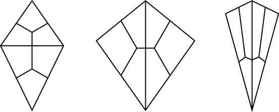
Figure 10: Kites divided into six quadrilaterals with no angle larger than $120^{\circ}$: (a) top and bottom angles both less than $120^{\circ}$; (b) top and bottom angles both greater than $60^{\circ}$; (c) top at least $120^{\circ}$ and bottom less than $120^{\circ}$.

Theorem 6

In $O(n\mathop{\rm log}n)$ time we can partition any polygon into a mesh of $O(n)$ quadrilaterals with maximum angle $120^{\circ}$.

Proof: The result follows from Theorem 4, since any kite (which we can assume without loss of generality to have a vertical axis of symmetry) can be divided into six $120^{\circ}$ quadrilaterals in one of three ways depending on how the top and bottom angles of the kite compare to $120^{\circ}$.

Specifically, we add new subdivision points on the midpoints of each kite edge. Then, if both the top and bottom angle of the kite are sharp (less than $120^{\circ}$), we can split the kite along a line between the left and right vertices, and subdivide both of the resulting triangles into three $120^{\circ}$ quadrilaterals (Figure 10(a)). If both angles are large (greater than $60^{\circ}$), we can similarly split the kite vertically along a line from top to bottom and again subdivide both of the resulting triangles (Figure 10(b)). In both of these two cases the subdivisions are axis-aligned or at $60^{\circ}$ angles to the axes. In the final case, the top angle is large (at least $120^{\circ}$) and the bottom is sharp (less than $120^{\circ}$). In this case, like the second, we partition the kite vertically into two triangles, and again partition each triangle into three; however in this final case the subdivisions are along lines between the bottom of the triangle and the two opposite edge midpoints, and at $60^{\circ}$ angles to those lines. It is easily verified that with the given assumptions on the angles of the original kite, all vertices of the subdivision lie as depicted in the figures and all angles are at most $120^{\circ}$.

7 Conclusions

We have shown that circle packing may be used in a variety of ways for quadrilateral mesh generation with simultaneous guaranteed bounds on complexity and quality.

Many questions remain open: How small can we make the constant factors in our complexity bounds, both in the worst case and in practice? Can we generate linear-complexity quadrilateral meshes with no small angles? Can we combine guarantees on several quality measures at once? Extensions of the circle packing method to three dimensional tetrahedral or hexahedral meshing would be of interest, but seem difficult due to the inability of three dimensional spheres to partition the domain into bounded-complexity regions. However perhaps our methods can be generalized to guaranteed-quality quadrilateral surface meshes.

Some of the methods we describe are purely of theoretical interest, due to high constant factors or distorted quadrilateral shapes, but we believe circle packing should be useful in practice as well. Among our methods, perhaps the low constant factors and lack of complicated cases in the Voronoï quadrilateralization make it the most practical choice.

References

References

- [1] I. Babuška and A. Aziz. On the angle condition in the finite element method. SIAM J. Numerical Analysis 13:214–227, 1976.
- [2] B. S. Baker, E. Grosse, and C. S. Rafferty. Nonobtuse triangulation of polygons. Discrete & Computational Geometry 3:147–168, 1988.
- [3] M. W. Bern, E. Demaine, D. Eppstein, and B. Hayes. A disk-packing algorithm for an origami magic trick. Proc. Int. Conf. Fun with Algorithms, 1998.
- [4] M. W. Bern and D. Eppstein. Polynomial-size nonobtuse triangulation of polygons. Int. J. Computational Geometry & Applications 2:241–255, 1992.
- [5] M. W. Bern and J. R. Gilbert. Drawing the planar dual. Inf. Proc. Lett. 43:7–13, 1992.
- [6] M. W. Bern, S. A. Mitchell, and J. Ruppert. Linear-size nonobtuse triangulation of polygons. Discrete & Computational Geometry 14:411–428, 1995.
- [7] T. D. Blacker and M. B. Stephenson. Paving: a new approach to automated quadrilateral mesh generation. Int. J. Numer. Meth. Engr. 32:811–847, 1991.
- [8] P. Doyle, Z.-X. He, and B. Rodin. Second derivatives of circle packings and conformal mappings. Discrete & Computational Geometry 11:35–49, 1994.
- [9] D. Eppstein. Faster circle packing with application to nonobtuse triangulation. Int. J. Computational Geometry & Applications 7(5):485–491, 1997.
- [10] R. Lang. A computational algorithm for origami design. Proc. 12th Symp. Computational Geometry, pp. 98–105. ACM, 1996.
- [11] G. L. Miller, D. Talmor, and S.-H. Teng. Optimal good-aspect-ratio coarsening for unstructured meshes. Proc. 8th Symp. Discrete Algorithms, pp. 538–547. ACM and SIAM, January 1997.
- [12] G. L. Miller, D. Talmor, S.-H. Teng, N. Walkington, and H. Wang. Control volume meshes using sphere packing: generation, refinement and coarsening. Proc. 5th Int. Meshing Roundtable, pp. 47–61. Sandia National Laboratories, October 1996, http://sass577.endo.sandia.gov/9225/Personnel/samitch/roundtable96/papers/miller-final2631.ps.gz.
- [13] M. Müller-Hannemann and K. Weihe. Minimum strictly convex quadrangulations of convex polygons. Proc. 13th Symp. Computational Geometry, pp. 183–202. ACM, June 1997.
- [14] L. R. Nackman and V. Srinivasan. Point placement for Delaunay triangulation of polygonal domains. Proc. 3rd Canad. Conf. Computational Geometry, pp. 37–40, 1991.
- [15] S. Ramaswami, P. Ramos, and G. Toussaint. Converting triangulations to quadrangulations. Proc. 7th Canad. Conf. Computational Geometry, pp. 297–302. Centre de recherche en géomatique, Université Laval, August 1995.
- [16] B. Rodin and D. Sullivan. The convergence of circle packings. J. Differential Geometry 26:349–360, 1987.
- [17] K. Shimada and D. C. Gossard. Bubble mesh: automated triangular meshing of non-manifold geometry by sphere packing. Proc. 3rd Symp. Solid Modeling & Applications, pp. 409–419. ACM, May 1995.
- [18] K. Stephenson. Approximation of conformal structures via circle packing. Proc. Computational Methods in Function Theory, 1997, http://www.math.utk.edu/~kens/ACS/ACS-revised.ps.gz.