The Distribution of Cycle Lengths in Graphical Models for Iterative Decoding

Abstract

This paper analyzes the distribution of cycle lengths in turbo decoding and low-density parity check (LDPC) graphs. The properties of such cycles are of significant interest in the context of iterative decoding algorithms which are based on belief propagation or message passing. We estimate the probability that there exist no simple cycles of length less than or equal to $k$ at a randomly chosen node in a turbo decoding graph using a combination of counting arguments and independence assumptions. For large block lengths $n$, this probability is approximately $e^{-\frac{2^{k-1}-4}{n}},k\geq 4$. Simulation results validate the accuracy of the various approximations. For example, for turbo codes with a block length of 64000, a randomly chosen node has a less than $1\%$ chance of being on a cycle of length less than or equal to 10, but has a greater than $99.9\%$ chance of being on a cycle of length less than or equal to 20. The effect of the “S-random” permutation is also analyzed and it is shown that while it eliminates short cycles of length $k<8$, it does not significantly affect the overall distribution of cycle lengths. Similar analyses and simulations are also presented for graphs for LDPC codes. The paper concludes by commenting briefly on how these results may provide insight into the practical success of iterative decoding methods.

1 Introduction

Turbo codes are a new class of coding systems that offer near optimal coding performance while requiring only moderate decoding complexity [1]. It is known that the widely-used iterative decoding algorithm for turbo codes is in fact a special case of a quite general local message-passing algorithm for efficiently computing posterior probabilities in acyclic directed graphical (ADG) models (also known as “belief networks”) [2, 3]. Thus, it is appropriate to analyze the properties of iterative-decoding by analyzing the properties of the associated ADG model.

In this paper we derive analytic approximations for the probability that a randomly chosen node in the graph for a turbo code participates in a simple cycle of length less than or equal to $k$. The resulting expressions provide insight into the distribution of cycle lengths in turbo decoding. For example, for block lengths of $64000$, a randomly chosen node in the graph participates in cycles of length less than or equal to $8$ with probability 0.002, but participates in cycles of length less than or equal to 20 with probability 0.9998.

In Section 2 we review briefly the idea of ADG models, define the notion of a turbo graph (and the related concept of a picture), and discuss how the cycle-counting problem can be addressed by analyzing how pictures can be embedded in a turbo graph. With these basic tools we proceed in Section 3 to obtain closed-form expressions for the number of pictures of different lengths. In Section 4 we derive upper and lower bounds on the probability of embedding a picture in a turbo graph at a randomly chosen node. Using these results, in Section 5 we derive approximate expressions for the probability of no simple cycles of length $k$ or less. Section 6 shows that the derived analytical expressions are in close agreement with simulation. In Section 7 we investigate the effect of the S-random permuter construction. Section 8 extends the analysis to LDPC codes and compares both analytic and simulation results on cycle lengths. Section 9 contains a discussion of what these results may imply for iterative decoding in a general context and Section 10 contains the final conclusions.

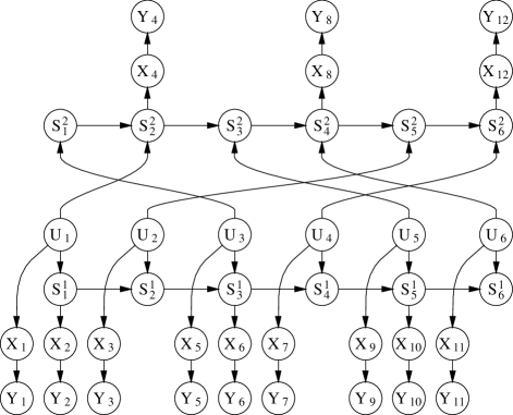
Figure 1: The ADG model for a $K=6,N=12$, rate $1/2$ turbocode.

2 Background and Notation

2.1 Graphical Models for Turbo-codes

An ADG model (also known as a belief network) consists of a both a directed graph and an associated probability distribution over a set of random variables of interest. There is a 1-1 mapping between the nodes in the graph and the random variables. Loosely speaking, the presence of a directed edge from node $A$ to $B$ in the graph means that $B$ is assumed to have a direct dependence on $A$ (“ $A$ causes $B$”). More generally, if we identify $\pi(A)$ as the set of all parents of $A$ in the graph (namely, nodes which point to $A$), then $A$ is conditionally independent of all other variables (nodes) in the graph (except for $A$’s descendants) given the values of the variables (nodes) in the set $\pi(A)$. For example, a Markov chain is a special case of such a graph, where each variable has a single parent. The general ADG model framework is quite powerful in that it allows us to systematically model and analyze independence relations among relatively large and complex sets of random variables [4].

As shown in [2, 3, 5], turbo codes can be usefully cast in an ADG framework. Figure 1 shows the ADG model for a rate $1/2$ turbo code. The $\rm{U}$ nodes are the original information bits to be coded, the $\rm{S}$ nodes are the linear feedback shift register outputs, the $\rm{X}$ nodes are the codeword vector which is the input to the communication channel, and the $\rm{Y}$ nodes are the channel outputs. The ADG model captures precisely the conditional independence relations which are implicitly assumed in the turbo coding framework, i.e., the input bits $\rm{U}$ are marginally independent, the state nodes $\rm{S}$ only depend on the previous state and the current input bit, and so forth.

The second component of an ADG model (in addition to the graph structure) is the specification of a joint probability distribution on the random variables. A fundamental aspect of ADG models is the fact that this joint probability distribution decomposes into a simple factored form. Letting $\{A_{1},\ldots,A_{n}\}$ be the variables of interest, we have

$$p(A_{1},\ldots,A_{n})=\prod_{i=1}^{n}p\left(A_{i}|\pi(A_{i})\right),$$ (1)

i.e., the overall joint distribution is the product of the conditional distributions of each variable $A_{i}$ given its parents $\pi(A_{i})$. (We implicitly assume discrete-valued variables here and refer to distributions; however, we can do the same factorization with density functions for real-valued variables, or with combinations of densities and distributions).

To specify the full joint distribution, it is sufficient to specify the individual conditional distributions. Thus, if the graph is sparse (few parents) there can be considerable savings in parameterization of the model. From a decoding viewpoint, however, the fundamental advantage of this factorization is that it permits the efficient calculation of posterior probabilities (or optimal bit decisions) of interest. Specifically, if the values for a subset of variables are known (e.g., the received codeword vector $\rm{Y}$) we can efficiently compute the posterior probability for the information bits $\rm{U_{i}}=1$, $1\leq i\leq N$. The power of the ADG framework is that there exist exact local message-passing algorithms which calculate such posterior probabilities. These algorithms typically have time complexity which is linear in the diameter of the underlying graph times a factor which is exponential in the cardinality of the variables at the nodes in the graph. The algorithm is provably convergent to the true posterior probabilities provided the graph structure does not contain any loops (a loop is defined as a cycle in the undirected version of the ADG, i.e., the graph where directionality of the edges is dropped). The message-passing algorithm of Pearl [6] was the earliest general algorithm (and is perhaps the best-known) in this general class of “probability propagation” algorithms. For regular convolutional codes, Pearl’s message passing algorithm applied to the convolutional code graph structure (e.g., the lower half of Figure 1) directly yields the BCJR decoding algorithm [7].

If the graph has loops then Pearl’s algorithm no longer provably converges, with the exception of certain special cases (e.g., see [8]). A “loop” is any cycle in the graph, ignoring directionality of the edges. The turbocode ADG of Figure 1 is an example of a graph with loops. In essence, the messages being passed can arrive at the same node via multiple paths, leading to multiple “over-counting” of the same information.

A widely used strategy in statistics and artificial intelligence is to reduce the original graph with loops to an equivalent graph without loops (this can be achieved by clustering variables in a judicious manner) and then applying Pearl’s algorithm to the new graph. However, if one applies this method to ADGs for realistic turbo codes the resulting graph (without loops) will contain at least one node with a large number of variables. This node will have cardinality exponential in this number of variables, leading to exponential complexity in the probability calculations referred to above. In the worst-case all variables are combined into a single node and there is in effect no factorization. Thus, for turbo codes, there is no known efficient exact algorithm for computing posterior probabilities (i.e., for decoding).

Curiously, as shown in [2, 3, 4], the iterative decoding algorithm of [1] can be shown to be equivalent to applying the local-message passing algorithm of Pearl directly to the ADG structure for turbo codes (e.g., Figure 1), i.e., applying the iterative message-passing algorithm to a graph with loops. It is well-known that in practice this decoding strategy performs very well in terms of producing lower bit error rates than any virtually other current coding system of comparable complexity. Conversely, it is also well-known that message-passing in graphs with loops can converge to incorrect posterior probabilities (e.g., [9]). Thus, we have the “mystery” of turbo decoding: why does a provably incorrect algorithm produce an extremely useful and practical decoding algorithm? In the remainder of this paper we take a step in understanding message-passing in graphs with loops by characterizing the distribution of cycle-lengths as a function of cycle length. The motivation is as follows: if it turns out that cycle-lengths are “long enough” then there may be a well-founded basis for believing that message-passing in graphs with cycles of the appropriate length are not susceptible to the “over-counting” problem mentioned earlier (i.e., that the effect of long loops in practice may be negligible). This is somewhat speculative and we will return to this point in Section 9. An additional motivating factor is that the characterization of cycle-length distributions in turbo codes is of fundamental interest by itself.

2.2 Turbo Graphs

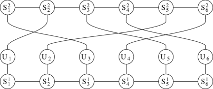
Figure 2: The cyclic graph structure underlying the turbo code of Figure 1

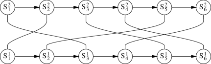
Figure 3: The underlying turbo graph for Figure 2.

In Figure 1 the underlying cycle structure is not affected by the $\rm{X}$ and $\rm{Y}$ nodes, i.e., they do not play any role in the counting of cycles in the graph. For simplicity they can be removed from consideration, resulting in the simpler graph structure of Figure 2. Furthermore, we will drop the directionality of the edges in Figure 2 and in the rest of the paper, since the definition of a cycle in an ADG is not a function of the directionality of the edges on the cycle.

To simplify our analysis further, we initially ignore the nodes $\rm{U_{1}}$, $\rm{U_{2}}$, $\ldots$, to arrive at a turbo graph in Figure 3 (we will later reintroduce the $\rm{U}$ nodes). Formally, a turbo graph is defined as follows:

1. There are two parallel chains, each having $n$ nodes. (For real turbo codes, $n$ can be very large, e.g. $n=64,000$.)

2. Each node is connected to one (and only one) node on the other chain and these one-to-one connections are chosen randomly, e.g., by a random permutation of the sequence $\{1,2,\ldots,n\}$. (In Section 7 we will look at another kind of permutation, the “S-random permutation.”)

3. A turbo graph as defined above is an undirected graph. But to differentiate between edges on the chains and edges connecting nodes on different chains, we label the former as being directed (from left to right), and the latter undirected. (Note: this has nothing to do with directed edges in the original ADG model, it is just a notational convenience.) So an internal node has exactly three edges connected to it: one directed edge going out of it, one directed edge going into it, and one undirected edge connecting it to a node on the other chain. A boundary node also has one undirected edge, but only one directed edge.

Given a turbo graph, and a randomly chosen node in the graph, we are interested in:

1. counting the number of simple cycles of length $k$ which pass through this node (where a simple cycle is defined as a cycle without repeated nodes), and

2. finding the probability that this node is not on a simple cycle of length $k$ or less, for $k=4,5,\ldots$ (clearly the shortest possible cycle in a turbo graph is 4).

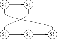
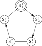
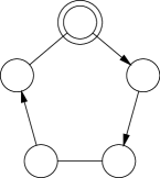
Figure 4: A simple cycle in Figure 3 and the corresponding picture (a) The simple cycle, (b) The same simple cycle, untangled, and (c) The corresponding picture.

2.3 Embedding “Pictures”

To assist our counting of cycles, we introduce the notion of a “picture.” First let us look at Figure 4, which is a single simple cycle taken from Figure 3. When we untangle Figure 4, we get Figure 4. If we omit the node labels, we have Figure 4 which we call a picture.

Formally, a picture is defined as follows:

1. It is a simple cycle with a single distinguished vertex (the circled one in the figure).

2. It consists of both directed edges and undirected edges.

3. The number of undirected edges $m$ is even and $m>0$.

4. No two undirected edges are adjacent.

5. Adjacent directed edges have the same direction.

We will use pictures as a convenient notation for counting simple cycles in turbo graphs. For example, using Figure 4 as a template, we start from node $\rm{S_{1}^{1}}$ in Figure 3. The first edge in the picture is a directed forward edge, so we go from $\rm{S_{1}^{1}}$ along the forward edge which leads us to $\rm{S_{2}^{1}}$. The second edge in the picture is also a directed forward edge, which leads us from $\rm{S_{2}^{1}}$ to $\rm{S_{3}^{1}}$. The next edge is an undirected edge, so we go from $\rm{S_{3}^{1}}$ to $\rm{S_{1}^{2}}$ on the other chain. In the same way, we go from $\rm{S_{1}^{2}}$ to $\rm{S_{2}^{2}}$, then to $\rm{S_{1}^{1}}$, which is our starting point. As the path we just traversed starts from $\rm{S_{1}^{1}}$ and ends at $\rm{S_{1}^{1}}$, and there are no repeated nodes in the path, we conclude that we have found a simple cycle (of length 5) which is exactly what we have in Figure 4.

We can easily enumerate all the different pictures of length $4,5,...,2n$, and use them as templates to find all the simple cycles at a node in a turbo graph. This approach is complete because any simple cycle in a graph has a corresponding picture. (To be exact, it has two pictures because we can traverse it in both directions.)

The process of finding a simple cycle using a picture as a template can also be thought of as embedding a picture at a node in a turbo graph. This embedding may succeed, as in our example above, or it may fail, e.g., we come to a previously-visited node other than the starting node, or we are told to go forward at the end of a chain, etc. Using pictures, the problem of counting the number of simple cycles of length $k$ can be formulated this way:

• Count the number of different pictures of length $k$,

• For each distinct picture, calculate the probability of embedding it in a turbo graph at a randomly chosen node.

3 Counting Pictures

We wish to determine the number of different pictures of length $k$ with $m$ undirected edges. First, let us define two functions:

$C(a,b)$

= the number of ways of picking $b$ disjoint edges (i.e., no two edges are adjacent to each other) from a cycle of length $a$, with a distinguished vertex and a distinguished clockwise direction.

$P(a,b)$

= the number of ways of picking $b$ independent edges from a path of length $a$, with a distinguished endpoint.

These two functions can be evaluated by the following recursive equations:

$$C(a,b) = P(a-1,b)+P(a-3,b-1)$$ (2)

$$P(a,b) = P(a-1,b)+P(a-2,b-1)$$ (3)

and the solutions are

$$P(a,b) = \left(\begin{array}[]{c}a-b+1\\ b\end{array}\right)$$ (6)

$$C(a,b) = \left(\begin{array}[]{c}a-b-1\\ b-1\end{array}\right)+\left(\begin{array}[]{c}a-b\\ b\end{array}\right)$$ (11)

Thus, the number of different pictures of length $k$ and with $m$ undirected edges, $0<m\leq\frac{n}{2}$ (and $m$ is even), is given by

$$N(k,m) = 2^{m}\left(\left(\begin{array}[]{c}k-m-1\\ m-1\end{array}\right)+\left(\begin{array}[]{c}k-m\\ m\end{array}\right)\right)/2$$ (16)

$$= 2^{m-1}\frac{k}{k-m}\left(\begin{array}[]{c}k-m\\ m\end{array}\right)$$ (19)

where $2^{m}$ is the number of different ways to give directions to the directed edges. The division by two occurs because the direction of the picture is irrelevant. Because of the $m$ undirected edges, there are $m$ segments of directed edges, with one or more edges in a segment; the edges within a segment must have a common direction (property 4 of a picture).

4 The Probability of Embedding a Picture

In this section we derive the probability $P_{n}(k,m)$ of embedding a picture of length $k$ and with $m$ undirected edges at a node in a turbo graph with chain length $n$.

4.1 When $k=2m$

Let us first consider a simple picture where the directed edges and undirected edges alternate (so $k=2m$) and all the directed edges point in the same (forward) direction.

Let us label the nodes of the picture as $X_{1}$,$X_{2}$,$Y_{1}$,$Y_{2}$, $X_{3}$,$X_{4}$,$Y_{3}$,$Y_{4}$,$\ldots$,
$X_{m-1}$,$X_{m}$,$Y_{m-1}$,$Y_{m}$. We want to see if this picture can be successfully embedded, i.e. if the above nodes are a simple cycle. Let us call the chain on which $X_{1}$ resides side 1, and the opposite chain side 2. The probability of successfully embedding the picture at $X_{1}$ is the product of the probabilities of successfully following each edge of the picture, namely,

• $X_{1}\rightarrow X_{2}$. This will fail if $X_{1}$ is the right-most node on side 1. So $p=1-\frac{1}{n}$.

• $X_{2}\rightarrow Y_{1}$. Here $p=1$.

• $Y_{1}\rightarrow Y_{2}$. This will fail if $Y_{1}$ is the right-most node on side 2. So $p=1-\frac{1}{n}$.

• $Y_{2}\rightarrow X_{3}$. $X_{3}$ is the “cross-chain” neighbor of $Y_{2}$. As there is already a connection between $X_{2}$ and $Y_{1}$, $X_{3}$ cannot possibly coincide with $X_{2}$; but it may coincide with $X_{1}$ and make the embedding fail. This gives us $p=1-\frac{1}{n-1}$.

  More generally, if there are $2s$ visited nodes on side 1, then $s$ of them already have their connections to side 2. So from a node on side 2, there are only $n-s$ nodes on side 1 to go to, $s$ of which are visited nodes. So $p=1-\frac{s}{n-s}$.

• $X_{3}\rightarrow X_{4}$. Here we have two previously visited nodes ($X_{1}$,$X_{2}$). When there are $2s$ previously-visited nodes, the unvisited nodes are partitioned into up to $s$ segments, and after we come from side 2 to side 1, if we fall on the right-most node of one of the segments, the embedding will fail: either we go off the chain, or we go to a previously-visited node. In this way, we have $1-\frac{s+1}{n-2s}\leq p\leq 1-\frac{1}{n-2s}$.

• $\cdots$

• $Y_{m-1}\rightarrow Y_{m}$.

• $Y_{m}\rightarrow X_{1}$. $p=\frac{1}{n-\frac{m}{2}}$. This final step ( $Y_{m}\rightarrow X_{1}$) completes the cycle.

Multiplying these terms, we arrive at

$$\frac{1}{n-\frac{m}{2}}\prod_{s=0}^{s=\frac{m}{2}}\left[\left(1-\frac{s}{n-s}\right)\left(1-\frac{s+1}{n-2s}\right)\right]^{2}$$

$$\leq P_{n}(k,m)$$

$$\leq \frac{1}{n-\frac{m}{2}}\prod_{s=0}^{s=\frac{m}{2}}\left[\left(1-\frac{s}{n-s}\right)\left(1-\frac{1}{n-2s}\right)\right]^{2}$$

For large $n$ and small $m$, the ratio between the upper bound and the lower bound is close to 1. For example, when $n=64,000$ and $m=10$ the ratio is $1.0005$.

4.2 The general case

The above analysis can be extended easily to the general case where:

• The directed edges in the picture are not constrained to be unidirectional.

• $k\geq 2m$. (Because the $m$ undirected edges cannot be adjacent to each other, the total number of edges $k$ must be $\geq 2m$.)

When $k=2m$, no two directed edges are adjacent. Equivalently, there are $m$ segments of directed edges, and in each segment, there is only one edge. When $k>2m$, we still have $m$ segments of directed edges, but there is more than one edge in a segment. Suppose for $1\leq i\leq m$, the $i$th segment of side 1 has $a_{i}$ edges, and the $i$th segment of side 2 has $b_{i}$ edges. $P_{n}(k,m)$ is given by:

$$\frac{1}{n-\frac{m}{2}}\prod_{s=0}^{s=\frac{m}{2}}\left[\left(1-\frac{\sum_{i=1}^{s}a_{i}}{n-s}\right)\left(1-\frac{s+1}{n-\sum_{i=1}^{s}(a_{i}+1)}\right)\left(1-\frac{\sum_{i=1}^{s}b_{i}}{n-s}\right)\left(1-\frac{s+1}{n-\sum_{i=1}^{s}(b_{i}+1)}\right)\right]$$

$$\leq P_{n}(k,m)$$

$$\leq \frac{1}{n-\frac{m}{2}}\prod_{s=0}^{s=\frac{m}{2}}\left[\left(1-\frac{\sum_{i=1}^{s}a_{i}}{n-s}\right)\left(1-\frac{1}{n-\sum_{i=1}^{s}(a_{i}+1)}\right)\left(1-\frac{\sum_{i=1}^{s}b_{i}}{n-s}\right)\left(1-\frac{1}{n-\sum_{i=1}^{s}(b_{i}+1)}\right)\right]$$

From

$$\sum_{i=1}^{m}a_{i}+\sum_{i=1}^{m}b_{i}=k-m,$$

$$1\leq a_{i},\,b_{i}\leq 1+(k-2m),$$

$$\sum_{i=1}^{s}a_{i}+\sum_{i=1}^{s}b_{i}\leq 2s+(k-2m),$$

and

$$s\leq\sum_{i=1}^{s}a_{i},\,\sum_{i=1}^{s}b_{i}\leq s+(k-2m)$$

we can simplify the bounds in Equation 4.2 to

$$\frac{1}{n-\frac{m}{2}}\prod_{s=0}^{s=\frac{m}{2}}\left[\left(1-\frac{s+k-2m}{n-s}\right)\left(1-\frac{s+1}{n-(2s+k-2m)}\right)\right]^{2}$$

$$\leq P_{n}(k,m)$$

$$\leq \frac{1}{n-\frac{m}{2}}\prod_{s=0}^{s=\frac{m}{2}}\left[\left(1-\frac{s}{n-s}\right)\left(1-\frac{1}{n-2s)}\right)\right]^{2}$$

The ratio between the upper bound and the lower bound is still close to 1. For example, when $n=64,000,k=10,m=4$, the ratio is $1.0003$. Given that the bounds are so close in the range of $n,k$, and $m$ of interest, in the remainder of the paper we will simply approximate $P_{n}(k,m)$ by the arithmetic average of the upper and lower bound.

5 The Probability of No Cycles of Length $k$ or Less

In Section 3 we derived $N(k,m)$, the number of different pictures of length $k$ with $m$ undirected cycles (Equation (19)). In Section 4 we estimated $P_{n}(k,m)$, the probability of embedding a picture (with length $k$ and $m$ undirected edges) at a node in a turbo graph with chain length $n$ (Equation (4.2)). With these two results, we can now determine the probability of no cycle of length $k$ or less at a randomly chosen node in a turbo graph of length $n$.

Let $P(\overline{{\cal L}_{k}})$ be the probability that there are no cycles of length $k$ at a randomly chosen node in a turbo graph. Thus,

$$P(no\ cycle\ of\ length\ \leq k) = P(\overline{{\cal L}}_{k},\overline{{\cal L}}_{k-1},\ldots,\overline{{\cal L}}_{4})$$ (23)

$$= \prod_{i=4}^{k}P(\overline{{\cal L}}_{i}\mid\overline{{\cal L}}_{i-1},\ldots,\overline{{\cal L}}_{4})$$

$$\approx \prod_{i=4}^{k}P(\overline{{\cal L}}_{i})$$

In this independence approximation we are assuming that at any particular node the event “there are no cycles of length $k$” is independent of the event “there are no cycles of length $k-1$ or lower.” This is not strictly true since (for example) the non-existence of a cycle of length $k-1$ can make certain cycles of length $k$ impossible (e.g., consider the case $k=5$). However, these cases appear to be relatively rare, leading us to believe that the independence assumption is relatively accurate to first-order.

Now we estimate $P(\overline{{\cal L}}_{k})$, the probability of no cycle of length $k$ at a randomly chosen node. Denote the individual pictures of length $k$ as $pic_{1}$,$pic_{2}$,$\ldots$, and let $\overline{pic}_{i}$ mean that the $i$th picture fails to be embedded.

$$P(\overline{{\cal L}}_{k}) = P(\overline{pic}_{1},\overline{pic}_{2},\ldots)$$ (24)

$$= \prod_{i}P(\overline{pic}_{i}\mid\overline{pic}_{i-1},\ldots,\overline{pic}_{1})$$

$$\approx \prod_{i}P(\overline{pic}_{i})$$

$$= \prod_{m>0,m\ even}^{m\leq\frac{k}{2}}\left(1-P_{n}(k,m)\right)^{N(k,m)}$$

Here we make a second independence assumption which again may be violated in practice. The non-existence of embedding of certain pictures (the event being conditioned on) will influence the probability of existence of embedding of other pictures. However, we conjecture that this dependence is rather weak and that the independence assumption is again a good first-order approximation.

6 Numerical and Simulation Results

k	$P_{simulation}$	$P_{theoretical}$	Difference	$\hat{\sigma}_{P}$
4	0.999950	0.999938	0.000012	0.000056
5	0.999750	0.999781	-0.000031	0.000105
6	0.999450	0.999500	-0.000050	0.000158
7	0.999100	0.999063	0.000037	0.000216
8	0.998350	0.998189	0.000161	0.000301
9	0.996650	0.996227	0.000423	0.000434
10	0.992400	0.992034	0.000366	0.000629
11	0.983750	0.983886	-0.000136	0.000890
12	0.968400	0.968456	-0.000056	0.001236
13	0.938850	0.938643	0.000207	0.001697
14	0.881800	0.880781	0.001019	0.002291
15	0.775350	0.774188	0.001162	0.002957
16	0.600550	0.598375	0.002175	0.003466
17	0.358850	0.358868	-0.000018	0.003392
18	0.125850	0.129488	-0.003638	0.002374
19	0.015500	0.016782	-0.001282	0.000908
20	0.000150	0.000279	-0.000129	0.000118

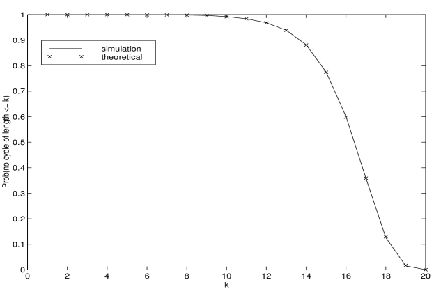
Figure 5: Theoretical vs. simulation estimates of the probability of no cycles of length $k$ or less, as a function of $k$. Turbo graph chain length $n=64,000$.

6.1 Cycle Length Distributions in Turbo Graphs

We ran a series of simulations where 200 different turbo graphs (i.e., each graph has a different random permuter) of length $n=64000$ are randomly generated. For each graph, we counted the simple cycles of length $k=4,5,\ldots,20$, at 100 randomly chosen nodes. In total, the cycle counts at $20000$ nodes are collected to generate an empirical estimate of the true $P(no~{}cycle~{}of~{}length~{}\leq~{}k)$. The theoretical estimates are derived by using the independence assumptions of Equations (23) and (24). $P_{n}(k,m)$ is calculated as the arithmetic average of the two bounds in Equation (4.2).

The simulation results, together with the theoretical estimates are shown in Figure 5. The difference in error is never greater than about 0.005 in probability. Note that neither the sample-based estimates nor the theoretical estimates are exact. Thus, differences between the two could be due to either sampling variation or error introduced by the independence assumptions in the estimation. The fact that the difference in errors is non-systematic (i.e., contains both positive and negative errors) suggests that both methods of estimation are fairly accurate. For comparison, in the last column of the table we provide the estimated standard deviation $\hat{\sigma}_{P}=\sqrt{\hat{P}(1-\hat{P})/N}$, where $\hat{P}$ is the simulation estimate. We can see that the differences between $P_{simulation}$ and $P_{theoretical}$ are within $\pm\hat{\sigma}_{P}$ of $P_{theoretical}$ except for the last three rows where $P_{theoretical}$ is quite small. For large $k$ we can expect that the simulation estimate of $\hat{P}$ will be less accurate since we are estimating relatively rare events. Thus, since our estimate of $\hat{\sigma}_{P}$ is a function of $\hat{P}$, for larger $k$ values any differences between theory and simulation could be due entirely to sampling error.

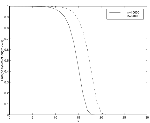
Figure 6: Approximate probability of no cycles of length $k$ or less, as a function of $k$.

Figure 6 shows a plot of the estimated probability that there are no cycles of length $k$ or less at a randomly chosen node. There appears to be a “soft threshold effect” in the sense that beyond a certain value of $k$, it rapidly becomes much more likely that there are cycles of length $k$ or less at a randomly chosen node. The location of this threshold increases as $n$ increases (i.e., as the length of the chain gets longer).

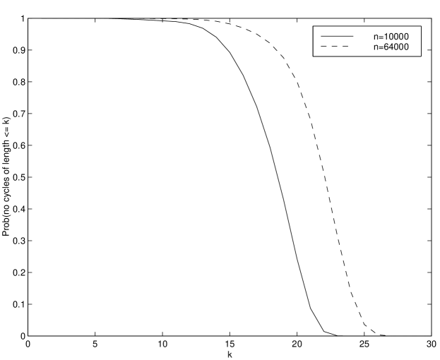
Figure 7: Probability of no cycles of length $k$ or less, including the $\rm{U}$ nodes (Figures 2) in the ADG for turbo decoding, as a function of $k$.

6.2 Large-Sample Closed-Form Approximations

When $n$ is sufficiently large, (i.e., $n\gg k$), the probability of embedding a picture (Equation (4.2)) can simply written as

$$P_{n}\approx\frac{1}{n}$$ (25)

In this case, we do not differentiate between pictures with different numbers of undirected edges

The total number of pictures of length $k$ is

$$N_{k} = \sum_{m>0,m\ even}^{m\leq\frac{k}{2}}N(k,m)$$ (28)

$$= \sum_{m>0,m\ even}^{m\leq\frac{k}{2}}2^{m-1}\frac{k}{k-m}\left(\begin{array}[]{c}k-m\\ m\end{array}\right)$$

$$\approx 2^{k-2}$$ (29)

The log probability of no cycle of length $k$ is then

$$\mathop{{\rm log}}P(\overline{{\cal L}}_{k})\approx\mathop{{\rm log}}(1-P_{n})^{N_{k}}\approx 2^{k-2}\mathop{{\rm log}}(1-\frac{1}{n})\approx-\frac{1}{n}2^{k-2},$$ (30)

from which one has

$$\mathop{{\rm log}}P(no\ cycle\ of\ length\ \leq k) \approx \mathop{{\rm log}}\left(\prod_{i=4}^{k}P(\overline{{\cal L}}_{i})\right)$$ (31)

$$\approx \sum_{i=4}^{k}\left(-\frac{1}{n}2^{i-2}\right)$$

$$= -\frac{2^{k-1}-4}{n}$$

Thus, the probability of no cycle of length $k$ or less is approximately $e^{-\frac{2^{k-1}-4}{n}},k\geq 4$. This probability equals 0.5 at $k_{0.5}=\mathop{{\rm log}}_{2}(n\mathop{{\rm log}}2+4)+1$, which provides an indication of how the curve will shift to the right as $n$ increases. Roughly speaking, to double $k_{0.5}$, one would have to square the block-length of the code from $n$ to $n^{2}$.

6.3 Including the $\rm{U}$ Nodes

Up to this point we have been counting cycles in the turbo graph (Figure 3) where we ignore the information nodes, $U_{i}$. The results can readily be extended to include these $\rm{U}$ nodes by counting each undirected edge (that connects nodes from different chains) as two edges.

Let $m^{\prime}=\frac{m}{2},\ k^{\prime}=k-\frac{m}{2}$ be the number of undirected edges and the cycle length, respectively, when we ignore the $\rm{U}$ nodes. From $m^{\prime}>0,\ m^{\prime}\ even,\ m^{\prime}\leq\frac{k^{\prime}}{2}$, we have $m>0,\ m\ divisible\ by\ 4,\ m\leq\frac{2k}{3}$.

Substituting these into Equation 24, we have

$$\prod_{m^{\prime}>0,m^{\prime}\ even}^{m^{\prime}\leq\frac{k^{\prime}}{2}}\left(1-P_{n}(k^{\prime},m^{\prime})\right)^{N(k^{\prime},m^{\prime})}$$ (32)

$$= \prod_{m>0,m\ divisible\ by\ 4}^{m\leq\frac{2k}{3}}\left(1-P_{n}\left(k-\frac{m}{2},\frac{m}{2}\right)\right)^{N(k-\frac{m}{2},\frac{m}{2})}$$

Using Equation 32, we plot in Figure 7 the estimated probability of no cycles of length $k$ or less in the graph for turbo decoding which includes the $\rm{U}$ nodes (Figure 2). Not surprisingly, the effect is to “shift” the graph to the right, i.e., adding $\rm{U}$ nodes has the effect of lengthening the typical cycle.

For the purposes of investigating the properties of the message-passing algorithm, the relevant nodes on a cycle may well be those which are directly connected to a $\rm{Y}$ node (for example, the $\rm{U}$ nodes in a systematic code and any $\rm{S}$ nodes which are producing a transmitted codeword). The rationale for including these particular nodes (and not including nodes which are not connected to a $\rm{Y}$ node) is that these are the only “information nodes” in the graph that in effect can transmit messages that potentially lead to multiple-counting. It is possible that it is only the number of these nodes on a cycle which is relevant to message-passing algorithms. Thus, for a particular code structure, the relevant nodes to count in a cycle could be redefined to be only those which have an associated $\rm{Y}$. The general framework we have presented here can easily be modified to allow for such counting.

Note also that various extensions of turbo codes are also amenable to this form of analysis. For example, for the case of a turbo code with more than two constituent encoders, one can generalize the notion of a picture and count accordingly.

7 The “S-random” permutation

In our construction of the turbo graph (Figure 3) we use a random permutation, i.e. the one-to-one connections of nodes from the two chains are chosen randomly by a random permutation. In this section we look at the “S-random” permutation [10], a particular semi-random construction.

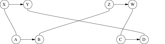
Figure 8: A cycle of length 8

Formally, the S-random permutation is a random permutation function $f(\cdot)$ on the sequence $1,2,\ldots,n$ such that

$$\forall i,j:\mid i-j\mid\leq S\,\,\Longrightarrow\,\,\mid f(i)-f(j)\mid\geq S$$ (33)

The S-random permutation stipulates that if two nodes on a chain are within a distance $S$ of each other, their counterparts on the other chain cannot be within a distance $S$ of each other. This restriction will eliminate some of the cycles occurring in a turbo graph with a purely random permutation. For example, there cannot be any cycles in the graph of length $k=$4, 5, 6 or 7. Thus, the S-random construction disallows cycles of length $k$ for $k<8$. However, from Section 6 we know that these short cycles ($k<8$) occur relatively rarely in realistic turbo codes. In Figure 8, we show a cycle of length $k=8$. As long as the distances of $\rm{\mid YZ\mid}$ and $\rm{\mid BC\mid}$ are large enough ($>S$), cycles of lengths $k\geq 8$ are possible for any $S$.

Prob(no cycle of length $k$ or less)
for turbo graph ($n=64000$)
	Random	S-random permutation
k	permutation	$S=10$	$S=20$	$S=50$	$S=100$
4	1.0000	1.0000	1.0000	1.0000	1.0000
5	0.9998	1.0000	1.0000	1.0000	1.0000
6	0.9995	1.0000	1.0000	1.0000	1.0000
7	0.9991	1.0000	1.0000	1.0000	1.0000
8	0.9984	0.9996	0.9998	0.9998	0.9998
9	0.9967	0.9983	0.9987	0.9987	0.9984
10	0.9924	0.9949	0.9945	0.9956	0.9950
11	0.9838	0.9890	0.9891	0.9877	0.9887
12	0.9684	0.9739	0.9765	0.9736	0.9748
13	0.9389	0.9460	0.9503	0.9449	0.9478
14	0.8818	0.8877	0.8920	0.8904	0.8913
15	0.7754	0.7804	0.7847	0.7858	0.7833
16	0.6006	0.6114	0.6014	0.6121	0.6006
17	0.3589	0.3671	0.3629	0.3731	0.3647
18	0.1259	0.1315	0.1289	0.1360	0.1330
19	0.0155	0.0146	0.0164	0.0184	0.0183
20	0.0002	0.0004	0.0003	0.0004	0.0008

Table 1: Simulation-based estimates of the probability of no cycle of length $k$ or less, comparing the standard random construction with the S-random construction.

We simulated S-random graphs and counted cycles in the same manner as described in Section 6, except that the random permutation was now carried out in the S-random fashion as described in [10]. The results in Table 1 show that changing the value of $S$ does not appear to significantly change the nature of the cycle-distribution. The S-random distributions of course have zero probability for $k<8$, but for $k\geq 8$ the results from both types of permutation appear qualitatively similar, with a small systematic increase in the probability of a node not having a cycle of length $k$ for the S-random case (relative to the purely random permutation). As the cycle-length $k$ increases, the difference between the S-random and random distributions narrow. For relatively short cycles with values of $k$ between 8 and 12 (say) the difference is relatively substantial if one considers the the probability of having a cycle of length less than or equal to $k$. For example, for $k=10$ and $S=100$, the S-random probability is 0.0050 while the probability for the random permuter is 0.0076 (see Table 1).

In [11, 12] it was shown (empirically) that the S-random construction does not have an “error floor” of the form associated with a random graph, i.e., the probability of bit error steadily decreases with increasing SNR for the S-random construction. The improvement in bit error rate is attributed to the improved weight distribution properties of the code resulting from the S-random construction. From a cycle-length viewpoint the S-random construction essentially only differs slightly from the random construction (e.g., by eliminating the relatively rare cycles of length $k=4,5,6$ and $7$). Note, however, that because two graphs have very similar cycle length distributions does not necessarily imply that they will have similar coding performance. It is possible that the elimination of the very short cycles combined with the small systematic increase in the probability of not having a cycle of length $k$ or less ($k\geq 8$), may be a contributing factor in the observed improvement in bit error rate, i.e., that even a small systematic reduction in the number of short cycles in the graph may translate into the empirically-observed improvement in coding performance.

8 Low-Density Parity Check Codes

LDPC codes are another class of codes exhibiting characteristics and performance similar to turbo codes [13, 14]. Like turbo codes, the underlying ADG has loops, rendering exact decoding intractable. Once again, however, iterative decoding (aka message-passing) works well in practice. Recent analyses of iterative decoding for LDPC codes have assumed that there are no short cycles in the LDPC graph structure [15, 16]. Thus, as with turbo codes, it is again of interest to investigate the distribution of cycle lengths for realistic LDPC codes.

The graph structure of regular LDPC codes is shown in Figure 9 (an LDPC graph). In this bipartite graph, at the bottom are $n$ variable nodes $\rm{v_{1}},\rm{v_{2}},\ldots,\rm{v_{n}}$, and at the top are the $w$ check nodes $\rm{c_{1}},\rm{c_{2}},\ldots,\rm{c_{w}}$. For the regular random LDPC construction each variable node has degree $d_{v}$, each check node has degree $d_{c}$ (obviously $nd_{v}=wd_{c}$), and the connectivity is generated in a random fashion.

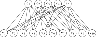
Figure 9: Graph structure of Low-Density Parity Check Codes: $d_{v}=3,d_{c}=6,n=10$.

Using our notion of a picture, we can also analyze the distribution of cycle lengths in LDPC graphs as we have done in turbo graphs. Obviously, here the cycle length must be even.

We define a picture for an LDPC graph as follows. Recall that in a turbo graph, the edges in a picture are labeled as undirected, forward, or backward. For an LDPC graph, we label an edge in a picture by a number $i$ between 1 and $d_{v}$ (or between 1 and $d_{c}$) to denote that this edge is the $i$-th edge coming from a node.

First consider the probability of successfully embedding a picture of length $k=2m$ at a randomly chosen node in an LDPC graph.

$$P_{embed}(k=2m) = 1\cdot(1-\frac{1}{d_{c}})\cdot(1-\frac{1}{d_{v}})$$

$$\cdot\left[(1-\frac{1}{d_{c}})(1-\frac{1}{n-1})\right]$$

$$\cdot\left[(1-\frac{1}{d_{v}})(1-\frac{1}{c-1})\right]$$

$$\cdot\left[(1-\frac{1}{d_{c}})(1-\frac{2}{n-1})\right]$$

$$\cdot\left[(1-\frac{1}{d_{v}})(1-\frac{2}{c-1})\right]$$

$$\cdots$$

$$\cdot\left[(1-\frac{1}{d_{c}})(1-\frac{m-2}{n-1})\right]$$

$$\cdot\left[(1-\frac{1}{d_{v}})(1-\frac{m-2}{c-1})\right]$$

$$\cdot\left[(1-\frac{1}{d_{c}})\frac{1}{n-1}\right]$$

$$= \frac{1}{n-1}\left(1-\frac{1}{d_{c}}\right)^{m}\left(1-\frac{1}{d_{v}}\right)^{m-1}\prod_{i=0}^{m-2}\left[\left(1-\frac{i}{n-1}\right)\left(1-\frac{i}{c-1}\right)\right]$$

The number of different pictures of length $k=2m$ is

$$N(k=2m)=\frac{1}{2}d_{c}^{m}d_{v}^{m}$$ (34)

Finally, the probability of no cycle of length $k=2m$ at a randomly chosen node in a LDPC graph is:

$$Prob(no\ cycle\ of\ length\ k=2m\ or\ less)$$

$$\approx \prod_{i=4,i\ even}^{k}Prob(no\ cycle\ of\ length\ i)$$

$$\approx \prod_{i=4,i\ even}^{k}\left(1-P_{embed}(i)\right)^{N(i)}$$

where we make the same two independence assumptions as we did for the turbo code case.

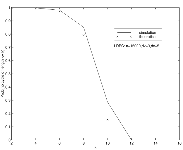
Figure 10: The probability of no cycles of length $k$ or less in an LDPC graph with $n=15000$, as a function of $k$.

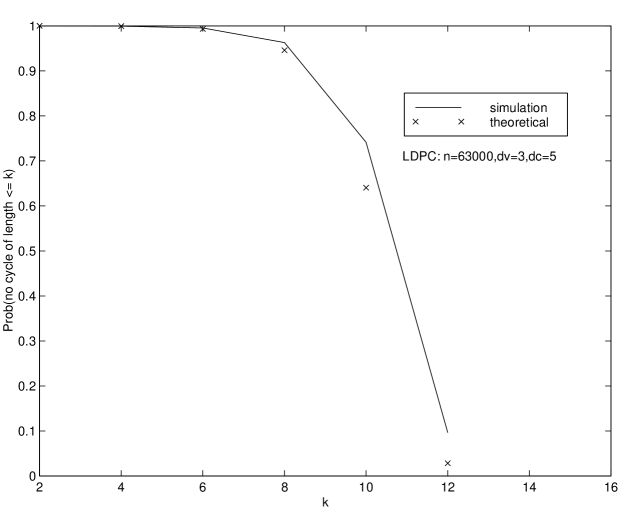
Figure 11: The probability of no cycles of length $k$ or less in an LDPC graph with $n=63000$, as a function of $k$.

We ran a number of simulations in which we randomly generated 200 different randomly generated LDPC graphs and counted the cycles at 100 randomly chosen nodes in each. We plot in Figures 10 and 11 the results of the simulation and the theoretical estimates from Equation 8 for $n=15000$ and 63000.

From the simulation results we see that the LDPC curve is qualitatively similar in shape to the turbo graph curves earlier but has been shifted to the left, i.e., there is a higher probability of short cycles in an LDPC graph than in a turbo graph, for the specific parameters we have looked at here. This is not surprising since the branching factor in a turbo graph is 3 (each node is connected to 3 neighbors) while the average branching factor in an LDPC graph (as analyzed with $d_{c}=5,d_{v}=3$) is 4.

Existing theoretical analyses of the message-passing algorithms for LDPC codes rely on the assumption that none of the cycles in the underlying graph are short [e.g., 15, 16]. In contrast, here we explicitly estimate the distribution on cycle lengths, and find (e.g., Figure 10 and 11) that there is a “soft threshold” effect (as with turbo graphs). For example, for $n=15000,d_{v}=3,d_{c}=5$, the simulation results in Figure 10 illustrate that the probability is about 50% that a randomly chosen node participates in a simple cycle of length 9 or less.

The independence assumptions clearly are not as accurate in the LDPC case as they were for the turbo graphs. Recall that we make two separate independence assumptions in our analysis, namely that

1. the event that there is no cycle of length $k$ is independent of the event that there are no cycles of length $k-1$ or lower, and

2. the event that a particular picture cannot be embedded at a randomly chosen node is independent of the event that other pictures cannot be embedded.

We can check the accuracy of the first independence assumption readily by simulation. We ran a number of simulations to count cycles in randomly generated turbo and LDPC graphs. From the simulation data, we estimate the marginal probabilities $P(\overline{{\cal L}}_{k})$, and the joint probabilities $P(\overline{{\cal L}}_{k},\overline{{\cal L}}_{k+1})$. To test the accuracy of our independence assumption, we compare the product of the estimated marginal probabilities with the estimated joint probability.

k	$P(\overline{{\cal L}}_{k})P(\overline{{\cal L}}_{k+1})$	$P(\overline{{\cal L}}_{k},\overline{{\cal L}}_{k+1})$	Difference
1	1.000000	1.000000	0.000000
2	1.000000	1.000000	0.000000
3	0.999950	0.999950	0.000000
4	0.999750	0.999750	0.000000
5	0.999500	0.999500	0.000000
6	0.999350	0.999350	0.000000
7	0.998900	0.998900	0.000000
8	0.997551	0.997550	0.000001
9	0.994007	0.994000	0.000007
10	0.986988	0.987050	-0.000062
11	0.975836	0.975850	-0.000014
12	0.954670	0.954500	0.000170
13	0.910886	0.910800	0.000086
14	0.826067	0.825350	0.000717
15	0.681002	0.679800	0.001202
16	0.460932	0.463650	-0.002718
17	0.213367	0.212600	0.000767
18	0.046814	0.046650	0.000164
19	0.002129	0.001350	0.000779

Table 2: Testing the independence between $\overline{{\cal L}}_{k}$ and $\overline{{\cal L}}_{k+1}$ in turbo graphs with chain length $n=64000$.

k	$P(\overline{{\cal L}}_{2k})P(\overline{{\cal L}}_{2k+2})$	$P(\overline{{\cal L}}_{k},\overline{{\cal L}}_{k+1})$	Difference
1	0.999542	0.999542	0.000000
2	0.995460	0.995458	0.000002
3	0.963715	0.963708	0.000007
4	0.746716	0.746771	-0.000055
5	0.097712	0.097333	0.000379

Table 3: Testing the independence between $\overline{{\cal L}}_{k}$ and $\overline{{\cal L}}_{k+1}$ in LDPC graphs with $n=63000,d_{v}=3,d_{c}=5$.

Table 2 provides the comparison for turbo graphs for $n=64000$. The products of the marginal probabilities are quite close to the joint probabilities, indicating that the independence assumption leads to a good approximation for turbo graphs. Table 3 gives a similar results for LDPC, i.e., the independence assumption appears quite accurate here also. Thus, we conclude that the first independence assumption (that the non-occurrence of cycles of length $k$ is independent of the non-occurrence of cycles of length $k-1$ of less) appears to be quite accurate for both turbo graphs and LDPC graphs.

Since assumption 2 is the only other approximation being made in the analysis of the LDPC graphs, we can conclude that it is this approximation which is less accurate (given that the approximation and simulation do not agree so closely overall for LDPC graphs). Recall that the second approximation is of the form:

$$P(\overline{{\cal L}}_{k}) = P(\overline{pic}_{1},\overline{pic}_{2},\ldots)$$

$$= \prod_{i}P(\overline{pic}_{i}\mid\overline{pic}_{i-1},\ldots,\overline{pic}_{1})$$

$$\approx \prod_{i}P(\overline{pic}_{i})$$

This assumption can fail for example when two pictures have the first few edges in common. If one fails to be embedded on one of these common edges, then the other will fail too. So the best we can hope from this approximation is that because there are so many pictures, these dependence effects will cancel out. In other words, we know that

$$P(\overline{pic}_{i})\neq P(\overline{pic}_{i}\mid\overline{pic}_{i-1},\ldots,\overline{pic}_{1})$$

but we hope that

$$P(\overline{pic}_{1},\overline{pic}_{2},\ldots)\approx\prod_{i}P(\overline{pic}_{i}).$$

One possible reason for the difference between the LDPC case and the turbo case is as follows. For turbo graphs, in the expression for the probability of embedding a picture,

$$P_{n}(k,m)\approx\frac{1}{n-\frac{m}{2}}\prod_{s=0}^{s=\frac{m}{2}}\left[\left(1-\frac{s}{n-s}\right)\left(1-\frac{1}{n-2s)}\right)\right]^{2}$$

the term $\frac{1}{n-\frac{m}{2}}$ is the most important, i.e., all other terms are nearly 1. So even if two pictures share many common edges and become dependent, as long as they do not share that most important edge, they can be regarded as effectively independent.

In contrast, for LDPC graphs, the contribution from the individual edges to the total probability tends to be more “evenly distributed.” Each edge contributes a $\left(1-\frac{1}{d_{c}}\right)$ term or a $\left(1-\frac{1}{d_{v}}\right)$ term. No single edge dominates the right hand side of

$$P_{embed}(k=2m)=\frac{1}{n-1}\left(1-\frac{1}{d_{c}}\right)^{m}\left(1-\frac{1}{d_{v}}\right)^{m-1}\prod_{i=0}^{m-2}\left[\left(1-\frac{i}{n-1}\right)\left(1-\frac{i}{c-1}\right)\right],$$

and, thus, the “effective independence” may not hold as in the case of turbo graphs.

9 Connections to Iterative Decoding

For turbo graphs we have shown that randomly chosen nodes are relatively rarely on a cycle of length 10 or less, but are highly likely to be on a cycle of length 20 or less (for a block length of 64000). It is interesting to conjecture about what this may tell us about the accuracy of the iterative message-passing algorithm in this context.

It is possible to show that there is a well-defined “distance effect” in message propagation for typical ADG models [17]. Consider a simple model where there is a hidden Markov chain consisting of binary-valued ${S_{i}}$ state nodes, $1\leq i\leq N$. In addition there is are observed $Y_{i}$, one for each state $S_{i}$ and which only depend directly on each state $S_{i}$. $p(Y_{i}|S_{i})$ is a conditional Gaussian with mean $S_{i}$ and standard deviation $\sigma$. One can calculate the effect of any observed $Y_{i}$ on any hidden node $S_{j}$, $j>i$, in terms of the expected difference between $p(S_{j}|Y_{j},\ldots,Y_{i+1})$ and $p(S_{j}|Y_{j},\ldots,Y_{i})$, averaged across many observations of the $Y$’s. This average change in probability, from knowing $Y_{i}$, can be shown to be proportional to $e^{-|i-j|}$, i.e., the effect of one variable on another dies off exponentially as a function of distance along the chain. Furthermore, one can show that as the channel becomes more reliable ($\sigma$ decreases), the dominance of local information over information further away becomes stronger, i.e., $Y_{i}$ has less effect on the posterior probability of $S_{j}$ on average.

The exponential decay of information during message propagation suggests that there may exist graphs with cycles where the information being propagated by a message-passing algorithm (using the completely parallel, or concurrent, version of the algorithm) can effectively “die out” before causing the algorithm to double count. Of course, as we have seen in this paper, there is a non-zero probability of cycles of length $k\geq 4$ for realistic turbo graphs, so that this line of argument is insufficient on its own to explain the apparent accuracy of iterative decoding algorithms.

It is also of interest to note that that iterative decoding has been empirically observed to converge to stable bit decisions within 10 or so. As shown experimentally in [5], even beyond 10 iterations of message-passing there are still a small fraction of nodes which typically change bit decisions. Combined with the results on cycle length distributions in this paper, this would suggest that it is certainly possible that double-counting is occurring at such nodes. It may be possible to show, however, that any such double-counting has relatively minimal effect on the overall quality of the posterior bit decisions.

10 Conclusions

The distributions of cycle lengths in turbo code graphs and LDPC graphs were analyzed and simulated. Short cycles (e.g., of length $k\leq 8$) occur with relatively low probability at any randomly chosen node. As the cycle length increases, there is a threshold effect and the probability of a cycle of length $k$ or less approaches 1 (e.g., for $k>20)$. For turbo codes, as the block length $n$ becomes large, the probability that a cycle of length $k$ or less exists at any randomly chosen node behaves approximately as $e^{-\frac{2^{k-1}-4}{n}},k\geq 4$. The S-random construction is shown to eliminate very short cycles and for larger cycles results in only a small systematic decrease in the probability of such cycles. For LDPC codes the analytic approximations are less accurate than for the turbo case (when compared to simulation results). Nonetheless the distribution as a function of $k$ shows qualitatively similar behavior to the distribution for turbo codes, as a function of cycle length $k$. In summary, the results in this paper demonstrate that the cycle lengths in turbo graphs and LDPC graphs have a specific distributional character. We hope that this information can be used to further understand the workings of iterative decoding.

References

1. C. Berrou, A. Glavieux, and P. Thitimajshima (1993). Near Shannon limit error-correcting coding and decoding: Turbo codes. Proceedings of the IEEE International Conference on Communications. pp. 1064-1070.

2. R.J. McEliece, D.J.C. MacKay, and J.-F. Cheng (1998). Turbo Decoding as an Instance of Pearl’s ‘Belief Propagation’ Algorithm. IEEE Journal on Selected Areas in Communications, SAC-16(2):140-152.

3. F. R. Kschischang, B. J. Frey (1998). Iterative Decoding of Compound Codes by Probability Propagation in Graphical Models. IEEE Journal on Selected Areas in Communications, SAC-16(2):219-230.

4. P. Smyth, D. Heckerman, and M. I. Jordan (1997). ‘Probabilistic independence networks for hidden Markov probability models,’ Neural Computation, 9(2), 227–269.

5. B. J. Frey (1998). Graphical Models for Machine Learning and Digital Communication. MIT Press: Cambridge, MA.

6. J. Pearl (1988), Probabilistic Reasoning in Intelligent Systems: Networks of Plausible Inference. Morgan Kaufmann Publishers, Inc., San Mateo, CA.

7. L. R. Bahl, J. Cocke, F. Jelinek, and J. Raviv (1974). ‘Optimal decoding of linear codes for minimizing symbol error rate,’ IEEE Transactions on Information Theory, 20:284–287.

8. Y. Weiss (1998). ‘Correctness of local probability propagation in graphical models with loops,’ submitted to Neural Computation.

9. R. J. McEliece, E. Rodemich, and J. F. Cheng, ‘The Turbo-decision Algorithm,’ in Proc. Allerton Conf. on Comm., Control, Comp., 1995.

10. S. Dolinar and D. Divsalar (1995), Weight Distributions for Turbo Codes Using Random and Nonrandom Permutations. TDA Progress Report 42-121 (August 1995), Jet Propulsion Laboratory, Pasadena, California.

11. R. G. Gallager (1963), Low-Density Parity-Check Codes. Cambridge, Massachusetts: MIT Press.

12. D.J.C. MacKay, R.M. Neal (1996), Near Shannon Limit Performance of Low Density Parity Check Codes, published in Electronics Letters, also available from http://wol.ra.phy.cam.ac.uk/.

13. K. S. Andrews, C. Heegard, and D. Kozen, (1998). ‘Interleaver Design Methods for Turbo Codes,’ Proceedings of the 1998 International Symposium on Information Theory, pg.420.

14. C. Heegard and S. B. Wicker (1998), Turbo Coding, Boston, MA: Kluwer Academic Publishers.

15. T. Richardson, R. Urbanke (1998), The Capacity of Low-Density Parity Check Codes under Message-Passing Decoding, preprint, available at
    http://cm.bell-labs.com/who/tjr/pub.html.

16. M. G. Luby, M. Mitzenmacher, M. A. Shokrollahi, D. A. Spielman (1998), ‘Analysis of Low Density Codes and Improved Designs Using Irregular Graphs,’ in Proceedings of the 30th ACM STOC. Also available online at
    http://www.icsi.berkeley.edu/ luby/index.html.

17. X. Ge and P. Smyth, ‘Distance effects in message propagation’, in preparation.