Setting Parameters by Example

Abstract

We introduce a class of “inverse parametric optimization” problems, in which one is given both a parametric optimization problem and a desired optimal solution; the task is to determine parameter values that lead to the given solution. We describe algorithms for solving such problems for minimum spanning trees, shortest paths, and other “optimal subgraph” problems, and discuss applications in multicast routing, vehicle path planning, resource allocation, and board game programming.

1 Introduction

Many cars now come equipped with route planning software that suggests a path from the current location to a desired destination. Similar services are also available on the internet (e.g., from http://maps.yahoo.com/). But although these routes may be found by computing shortest paths in a graph representing the local road system, the “distance” may be a weighted sum of several values other than actual mileage: expected travel time, scenic value, number of turns, tolls, etc. [19]. Different drivers may have different preferences among these values, and may not be able to clearly articulate these preferences. Can we automatically infer the appropriate weights to use in the sum by observing the routes actually chosen by a driver?

More abstractly, we define an inverse parametric optimization problem as follows: we are given as input both a parametric optimization problem (that is, a combinatorial optimization problem such as shortest paths, but with the element weights being linear combinations of certain parameters rather than fixed numbers), and also a desired optimal solution for the problem. Our task is to determine parameter values such that the given solution is optimal for those values.

Along with the path planning problem described above, one can find many other applications in which one must tune the parameters to an optimization problem:

• In many online services such as web page hosting, data is sent in a star topology from a central server to each user. But in multicast routing of video and other high-bandwidth information, network resources are conserved by sending the data along the edges of a tree, in which some users receive copies of the data from other users rather than from the central server. Natural measures of the quality of each edge in this routing tree include the edge’s bandwidth, congestion, delay, packet loss, and possibly monetary charges for use of that link. Since one can find minimum spanning trees efficiently in the distributed setting [8], it is natural to try to model this routing problem using minimum spanning trees. Given one or more networks with these parameters, and examples of desired routing trees, how can we set the weights of each quality measure so that the desired trees are the minimum spanning trees of their networks?

• Bipartite matching, or the assignment problem, is a common formalism for grouping indivisible resources with resource consumers. For instance, the first example given for matching by Ahuja et al. [2] is to assign recently hired workers to jobs, using weights based on such values as aptitude test scores and college grades. One might set the weight of an edge from worker $i$ to job $j$ to be $a_{i}\cdot p_{j}$, where $a_{i}$ is the (known) set of aptitudes of the worker, and $p_{j}$ is the (unknown) set of parameters describing the combination of aptitudes best fitting the job. Again, it is natural to ask for a way to automatically set the parameters of each job, based on experience assigning previously hired workers to those jobs.

• Many board games, such as chess, checkers, or Othello, can be played well by programs based on relatively simple alpha-beta searching algorithms. However, these programs use relatively complex evaluation functions in which the evaluation of a given position can be the sum of hundreds or thousands of terms. Some of these terms may represent the gross material balance of a game (e.g., in chess, one usually normalizes the score so that a pawn is worth 1 point, while a knight may be worth 2.5-3 points) while others represent more subtle features of piece placement, king safety, advanced pawns, etc. The weight of each of these terms may be individually adjusted in order to improve the quality of play. Although there have been some preliminary experiments in using evolutionary learning techniques to tune these weights [21], they are currently usually set by hand. The true test of a game program is in actual play, but programs are also often tuned by using test suites, large collections of positions for which the correct move is known. If we are given a test suite, can we automatically set evaluation weights in such a way that a shallow alpha-beta search can find each correct move?

1.1 New Results

We show the following theoretical results:

• For the inverse parametric minimum spanning tree problem, in the case that the number of parameters is a fixed constant, we provide a randomized algorithm with linear expected running time, and a deterministic algorithm with worst case running time $O(m\mathop{\rm log}^{2}n)$.

• For the minimum spanning tree, shortest path, matching, and other “optimal subgraph” problems for which the optimization problem can be solved in polynomial time, we show that the inverse optimization problem can also be solved in polynomial time by means of the ellipsoid method from linear programming, even when the number of parameters is large.

In addition, although we do not provide theoretical results for this case, we discuss the game tree search problem and describe how to fit it into the same inverse parametric optimization framework.

In cases where the initial problem is infeasible (there is no parameter setting leading to the desired optimum), our techniques provide a witness for infeasibility: a small number of alternative solutions, one of which must be better than the given solution for any parameter setting. One can then examine these solutions to determine whether the initial solution is suboptimal or whether additional parameters should be added to better model the users’ utility functions.

1.2 Relation to Previous Work

Although there has been considerable work on parametric versions of optimization problems such as minimum spanning trees [1] and shortest paths [23], we are not aware of any prior work in inverting such problems to produce parameter values that match given solutions. One could compute the set of solutions available over the range of parameter values, and compare these solutions to the given one, but the number of different solutions would typically grow exponentially with the number of parameters.

The inverse parametric optimization problems considered here are most closely related to parametric search, which describes a general class of problems in which one sets the parameters of a parametric problem in order to optimize some criterion. However in most applications of parametric search, the criterion being optimized is a numeric function of the solution (e.g. the ratio between two linear weights) rather than the solution structure itself. Megiddo [16] describes a very general technique for solving parametric search problems, in which one simulates the steps of an optimization algorithm, at each conditional step using the algorithm itself as an oracle to determine which conditional branch to take. However this technique does not seem to apply to our problems, because the given optimal structure (e.g. a single shortest path) does not give enough information to deduce the conditional branches followed by a shortest path algorithm.

The vehicle routing problem discussed in the introduction was introduced by Rogers and Langley [19]. However, they used a weaker model of optimization (a hill-climbing procedure) and a stronger model of user interaction requiring the user to specify preferences in a sequence of choices between pairs of routes.

2 Minimum Spanning Trees

In this section, we consider the inverse parametric minimum spanning tree problem, in which we are given a fixed tree $T$ in a network in which the weight of each edge $e$ is a linear function $w(e)={\rm\bf c}_{e}\cdot{\rm\bf p}$ (where ${\rm\bf p}$ represents the unknown vector of parameter settings and ${\rm\bf c}_{e}$ represents the known value of edge $e$ according to each parameter). Our task is to find a value of ${\rm\bf p}$ such that $T$ is the unique minimum spanning tree for the weights $w(e)$.

If we fix a given spanning tree $T$ in a network, a pair of edges $(e,f)$ is defined to be a swap if $T\cup\{f\}-\{e\}$ is also a spanning tree; that is, if $e$ is an edge in $T$, $f$ is not an edge in $T$, and $e$ belongs to the cycle induced in $T$ by $f$. $T$ is the unique minimum spanning tree if and only if for every swap $(e,f)$, the weight of $f$ is greater than the weight of $e$.

Thus we can solve the inverse parametric minimum spanning tree problem as a linear program, in which we have one variable per parameter, and one constraint $({\rm\bf c}_{f}-{\rm\bf c}_{e})\cdot{\rm\bf p}>0$ per swap. If the number of variables is a fixed constant, a linear program may be solved in time linear in the number of constraints [17]; however here the number of constraints may be $\Theta(m\kern 1.00006ptn)$.

We show how to improve this by a randomized algorithm which takes linear time and a deterministic algorithm which takes time $O(m\mathop{\rm log}^{2}n)$. Both algorithms are based on (different) random sampling schemes for low dimensional linear programming, due to Clarkson [3].

2.1 Randomized Spanning Tree Algorithm

Clarkson [3] showed that, if one randomly samples $k$ constraints from a $d$-dimensional linear program with $n$ constraints, and computes the optimum for the subprogram consisting only of the sampled constraints, then the expected number of the remaining constraints violated by this optimum is at most $d(n-k)/(k+1)$. Further, if any constraint is violated, at least one of the $d$ constraints involved in any base (minimal subset of constraints having the same solution as the overall problem) belongs to the set of violated constraints. If no constraint is violated, the problem is solved.

This suggests the following randomized algorithm for the inverse parametric minimum spanning tree problem, where $d=O(1)$ is a fixed constant. We define a potential swap for the given tree $T$ to be a pair $(e,f)$ where $e$ belongs to $T$ and $f$ does not, regardless of whether $(e,f)$ is actually a swap. For technical reasons, we need to define a unique optimal parameter setting ${\rm\bf p}$ for any subset of constraints, which we achieve by introducing an arbitrary linear objective function.

1. Let set $S$ be initialized to empty.

2. Repeat $d$ times:

   1. Let set $R$ be a random sample of $d\sqrt{m\kern 1.00006ptn}$ potential swaps.

   2. Find the optimal parameter setting ${\rm\bf p}$ for constraints from $R\cup S$.

   3. Add the constraints violated by ${\rm\bf p}$ to $S$.

3. Find the optimal parameter setting ${\rm\bf p}$ for constraints from $S$.

Each iteration increases the size of the intersection of $S$ with the optimal base, so the loop terminates with a correct solution. The expected number of edges added to $S$ in each iteration is $O(\sqrt{m\kern 1.00006ptn})$, so the expected size of $S$ is $O(d\sqrt{m\kern 1.00006ptn})=O(m)$. If $d=O(1)$, the step in which we find ${\rm\bf p}$ can be performed in time $O(d\sqrt{m\kern 1.00006ptn})=O(m)$ by fixed dimensional linear programming techniques. It remains to determine how we tell whether a potential swap $(e,f)$ is really a swap (so we can determine whether to use it as a constraint or ignore it in step (b)), and how to find the set of violated constraints (step (c)).

To test a potential swap, we simply build a least common ancestor data structure [20] on the given tree $T$ (with an arbitrary choice of root). The pair $(e,f)$ is a swap if both endpoints of $e$ are on the path from one of the endpoints of $f$ to the common ancestor of the two endpoints.

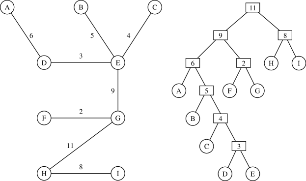
Figure 1: (a) A weighted tree $T$; (b) Auxiliary tree used to find heaviest edges on paths in $T$.

To find the violated constraints for ${\rm\bf p}$, we also use least common ancestors, on an auxiliary tree in which internal nodes represent edges and leaves represent vertices of $T$ (Figure 1). We build this auxiliary tree by choosing the root to be the maximum weight edge $e$ (according to ${\rm\bf p}$) in $T$, with the two children of the root being auxiliary trees constructed recursively on the two components of $T-\{e\}$. This construction takes time $O(n\mathop{\rm log}n)$. The least common ancestor of two leaves in this auxiliary tree represents the maximum weight edge on the path between the corresponding vertices of $T$. Therefore, if $f$ is a given non-tree edge, we can find a swap $(e,f)$ giving a violated constraint (if one exists) by using this auxiliary tree to find the maximum weight edge on the path between $f$’s endpoints. If this gives us a violated swap, we continue recursively on the subpaths between $f$ and the endpoints of $e$, until all swaps involving $f$ have been listed. Each swap is found in $O(1)$ time, and the expected number of swaps corresponding to violated constraints is $O(\sqrt{m\kern 1.00006ptn})$, so the total expected time for this procedure (including the time to construct the auxiliary tree) is $O(m+n\mathop{\rm log}n)$.

Lemma 1

We can solve the inverse parametric minimum spanning tree problem, for any constant number of parameters, in randomized expected time $O(m+n\mathop{\rm log}n)$.

In order to remove the unnecessary logarithmic factor from this bound, we resort to another round of sampling. However this time we sample tree edges rather than swaps.

Lemma 2

Let $S$ be a randomly chosen sample of $k$ edges from tree $T$, let graph $G^{\prime}$ and tree $T^{\prime}$ be formed from $G$ and $T$ respectively by contracting the edges in $T-S$, and let ${\rm\bf p}$ be the optimal parameter setting for the inverse parametric minimum spanning tree problem defined by $G^{\prime}$ and $T^{\prime}$. Then the expected number of the remaining edges of $T$ that take part in a constraint violated by this optimum is at most $d(n-k-1)/(k+1)$.

Proof: Consider selecting $S$ in the following way: choose a random permutation on the edges of $T$, and let $S$ be the first $k$ edges in the permutation. Let $e$ be the $(k+1)$st edge in the permutation. Then since $e$ is equally likely to be any remaining edge, the expected number of edges that take part in a violated constraint is just $n-d-1$ times the probability that $e$ takes part in a violated constraint. But this can only happen if $e$ is one of the at most $d$ edges involved in the optimal base for $S\cup\{e\}$. Since this subset is just the first $k+1$ edges in the permutation, and any permutation of this subset is equally likely, this probability is at most $d/(k+1)$.

Thus we can apply the following algorithm:

1. Let set $S$ be initialized to empty.

2. Repeat $d$ times:

   1. Let set $R$ be a random sample of $d\sqrt{n}$ edges of $T$.

   2. Contract the edges in $T-(R\cup S)$ to produce $T^{\prime}$ and $G^{\prime}$.

   3. Find the optimal parameter setting ${\rm\bf p}$ for $T^{\prime}$ and $G^{\prime}$ using the algorithm of Lemma 1.

   4. Add to $S$ the tree edges that take part in a constraint violated by ${\rm\bf p}$.

3. Contract the edges in $T-S$ to produce $T^{\prime}$ and $G^{\prime}$.

4. Find the optimal parameter setting ${\rm\bf p}$ for $T^{\prime}$ and $G^{\prime}$ using the algorithm of Lemma 1.

The arguments for termination and correctness are the same as before. It remains to explain how we find the set of violated tree edges. This can be done in time $O(m\alpha(m,n))$ by an algorithm of Tarjan [22], but using this algorithm directly would lead to a nonlinear overall time bound. More recent minimum spanning tree verification algorithms [4, 13] can be used to find the violated non-tree edges, but not the tree edges. However, in our case we can perform this verification task efficiently due to the expected small number of differences between $T$ and the minimum spanning tree for ${\rm\bf p}$.

Lemma 3

In the algorithm above, the tree edges that take part in a violated constraint can be found in expected linear time.

Proof: We use the linear time randomized minimum spanning tree algorithm of Karger et al. [11], and let $X$ denote the set of edges that are in the MST and not in $T$. Note that $X$ has exactly as many edges as are in $T$ and not in the MST; since each edge in the latter set takes part in a violated swap constraint, the expectation of $|X|$ is $O(\sqrt{n})$ by Lemma 2. Then it is easy to see that, if tree edge $e$ takes part in any violated constraints, at least one must be the constraint corresponding to swap $(e,f)$, where $f$ is the minimum weight edge in $X$ forming a swap with $e$.

To find this minimum weight swap for each tree edge, we contract $T$ as follows. While $T$ has a degree-one vertex that is not adjacent to any edge in $X$, we remove it and its incident edge; that edge can not take part in any swaps with $X$. While $T$ has a degree-two vertex that is not adjacent to any edge in $X$, we remove it and merge its two incident edges into a single edge; these two edges share the same minimum swap edge.

After this contraction process, the contracted tree $T^{\prime}$ has $O(|X|)$ vertices with degree less than three, and therefore $O(|X|)$ total vertices. We apply Tarjan’s nonlinear minimum spanning tree verification algorithm to this contracted tree to find the best swap in $X$ for each contracted tree edge. We then undo the contraction process and propagate the best swap information to the original tree edges. Finally, once we have computed the best swap $(e,f)$ for each tree edge $e$, we simply compute $w(e)$ and $w(f)$ and compare the two weights to determine whether this swap leads to a violated constraint.

Theorem 1

We can solve the inverse parametric minimum spanning tree problem, for any constant number of parameters, in randomized linear expected time.

Proof: The problem is solved by the algorithm above. In each iteration the expected size of the set added to $S$ is $O(\sqrt{n})$, so the total size of $R\cup S$ is $O(d\sqrt{n})=O(\sqrt{n})$. In each iteration we add one more member of the optimal base to $S$, so the algorithm terminates with the correct solution. The steps in which we find the optimal parameter setting for $T^{\prime}$ and $G^{\prime}$ can be performed by applying Lemma 1; since $T^{\prime}$ has $O(\sqrt{n})$ edges, the time for these steps is $O(m+\sqrt{n}\mathop{\rm log}n)=O(m)$. The step in which we find the edges that take part in a violated constraint can be performed in linear expected time by Lemma 3.

2.2 Deterministic Spanning Tree Algorithm

To solve the inverse parametric minimum spanning tree problem deterministically, we derandomize a different sampling technique also based on a method of Clarkson [3]. However, as in our randomized algorithm, we modify this technique somewhat by sampling edges instead of constraints.

We begin by applying the multi-level restricted partition technique of Frederickson [6, 7] to the given tree $T$.

               

Figure 2: (a) Restricted partition of order 2; (b) multi-level partition.

By introducing dummy edges, we can assume without loss of generality that $T$ is binary and that the root $t$ of $T$ has indegree one. These dummy edges will only be used to form the partition and will not take part in the eventual optimization procedure.

Definition 1

A restricted partition of order $z$ with respect to a rooted binary tree $T$ is a partition of the vertices of $V$ such that:

1. Each set in the partition contains at most $z$ vertices.

2. Each set in the partition induces a connected subtree of $T$.

3. For each set $S$ in the partition, if $S$ contains more than one vertex, then there are at most two tree edges having one endpoint in $S$.

4. No two sets can be combined and still satisfy the other conditions.

Such a partition (for $z=2$) is depicted in Figure 2(a). In general such a partition can easily be found in linear time by merging sets until we get stuck. Alternatively, by working bottom up we can find an optimal partition in linear time. We will defer until later choosing a value for $z$; for now we leave it as a free parameter.

Lemma 4 (Frederickson [7])

Any order-$z$ partition of a binary tree $T$ has $O(n/z)$ sets in the partition. For $z=2$ we can find a partition with at most $5n/6$ sets.

Contracting each set in a restricted partition gives again a binary tree. We form a multi-level partition [7] by recursively partitioning this contracted binary tree (Figure 2(b)).

We now use these partitions to construct a set $\Pi$ of paths in $T$. We include in $\Pi$ the path in $T$ between any two vertices that are in the same set at some level of the partition. Note that, although the vertices at higher levels of the partition correspond to contracted subtrees of $T$, the path in $T$ between two such subtrees can still be unambiguously defined.

Lemma 5

The set of paths defined above has the following properties:

• There are $O(n\kern 1.00006ptz)$ paths.

• Each edge in $T$ belongs to $O(z^{2}\mathop{\rm log}_{z}n)$ paths.

• Any path in $T$ can be decomposed into the disjoint union of $O(\mathop{\rm log}_{z}n)$ paths.

Proof: The first property follows immediately from Lemma 4, since each set of the partition contributes $O(z^{2})$ paths, there are $O(n/z)$ sets at the bottom level of the partition, and the number of sets decreases at least geometrically at each level. Similarly, the second property follows, since an edge can belong to $O(z^{2})$ paths per level and there are $O(\mathop{\rm log}_{z}n)$ levels.

Finally, to prove the third property, let $p$ be an arbitrary path in $T$. We describe a procedure for decomposing $p$ into few paths $\pi_{i}\in\Pi$. More generally, suppose we have a path $p$ contained in a set $S$ at some level of a multi-level decomposition (note that the whole tree is the set at the highest level of the partition). Then $S$ can be decomposed into at most $z$ sets at the next level of the partition; $p$ has endpoints in at most two of these sets, and may pass completely through some other sets. Therefore, $p$ can be decomposed into the union of two smaller paths in the sets containing its endpoints, together with a single path $\pi_{i}$ connecting those two sets. By repeating this decomposition recursively at each level of the tree, we obtain a decomposition into at most two paths per level, or $O(\mathop{\rm log}_{z}n)$ paths overall.

We now describe how to use this path decomposition in our inverse optimization problem. For each path $\pi_{i}\in\Pi$, let $A_{i}$ denote the set of edges in $T$ belonging to $\pi_{i}$, and let $B_{i}$ denote the set of edges in $G-T$ such that $\pi_{i}$ is part of the decomposition of the tree path between each edge’s endpoints. The total size of all the sets $A_{i}$ and $B_{i}$ is $O((m+n\kern 1.00006ptz^{2})\mathop{\rm log}_{z}n)$, and all sets can be constructed in time linear in their total size.

A pair $(e,f)$ is a swap if and only if there is some $e$ for which $e\in A_{i}$ and $f\in B_{i}$. With this decomposition, the inverse parametric minimum spanning tree problem becomes equivalent to asking for a parameter ${\rm\bf p}$ such that, for each $i$, the weight of every member of $A_{i}$ is less than the weight of every member of $B_{i}$.

For a single value of $i$, one could solve such a problem by a $(d+1)$-dimensional linear program in which we augment the parameters by an additional variable that is constrained to be greater than each $e\in A_{i}$ and less than each $f\in B_{i}$, however adding a separate variable for each $i$ would make the dimension nonconstant.

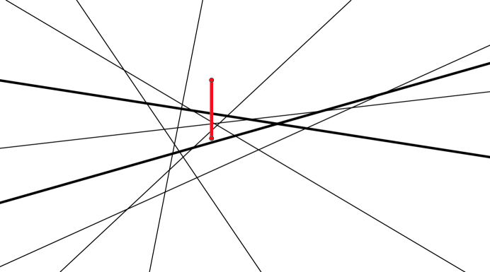
Figure 3: Example $\epsilon$-net, for $\epsilon=1/2$: every vertical line segment that crosses $\geq n/2$ lines in the overall arrangement also crosses at least one of the two heavy lines.

Instead, we use a standard derandomization technique from computational geometry, $\epsilon$-nets. If we graph the weight of each edge in a $(d+1)$-dimensional space, where the parameter values are independent variables and the weight is the dependent variable, the result is a hyperplane. For any set $S$ of these hyperplanes, and any $\epsilon>0$, define an $\epsilon$-net for vertical line segments to be a subset $S^{\prime}$ such that, if any vertical line segment intersects at least $\epsilon|S|$ hyperplanes in $S$, the same segment must intersect at least one hyperplane in $S^{\prime}$ (Figure 3). More generally, if the members of $S$ are given costs, an $\epsilon$-net must contain at least one member of any subset that is formed by intersecting the hyperplanes with a vertical segment and that has total cost at least $\epsilon$ times the total cost of $S$. If $1/\epsilon=O(1)$, an $\epsilon$-net of size $O(1)$ can be found in time linear in $|S|$ [14].

Our algorithm can then be described as follows. We will use $\epsilon=1/3d$.

1. Use a recursive partition to find the sets $A_{i}$ and $B_{i}$.

2. Assign unit cost to each edge in the graph.

3. Repeat until terminated:

   1. Construct $\epsilon$-nets $A^{\prime}_{i}$ and $B^{\prime}_{i}$ for each $A_{i}$ and $B_{i}$.

   2. Let $S$ be the set of swaps involving only $\epsilon$-net members. Find the optimal parameter setting ${\rm\bf p}$ for constraints from $S$.

   3. Find the maximum weight $a_{i}$ of an edge in each $A_{i}$ and the minimum weight $b_{i}$ of an edge in each $B_{i}$, where weights are measured according to ${\rm\bf p}$. If $a_{i}<b_{i}$ for each $i$, terminate the algorithm.

   4. Find the maximum weight $a^{\prime}_{i}$ of an edge in each $A^{\prime}_{i}$ and the minimum weight $b^{\prime}_{i}$ of an edge in each $B^{\prime}_{i}$. Double the cost of each edge in $A_{i}$ with $w(e)>a^{\prime}_{i}$, and each edge in $B_{i}$ with $w(e)<b^{\prime}_{i}$.

The set of edges in $A_{i}$ for which the costs are doubled is defined by the intersection of $A_{i}$ with a vertical line segment: the segment with parameter coordinates ${\rm\bf p}$ and with weight coordinate beween $a^{\prime}_{i}$ and $\infty$. It does not contain any member of $A^{\prime}_{i}$, so it must have total cost at most $\epsilon$ times the cost of $A_{i}$. Therefore each iteration increases the total cost of all the sets $A_{i}$ (and similarly $B_{i}$) by a factor of at most $1+\epsilon=1+1/3d$.

If there is any constraint violated by the solution ${\rm\bf p}$, then at least one violated constraint must be a member of the $d$-swap base defining the optimal overall solution. Note however that, in any iteration of the loop, $a^{\prime}_{i}<b^{\prime}_{i}$ because of how we computed ${\rm\bf p}$, so any violated constraint coming from a swap $(e,f)$ must have $w(e)>a^{\prime}_{i}$ or $w(f)<b^{\prime}_{i}$. Therefore at least one of the $2d$ edges involved in the optimal base must have its cost doubled, and the cost of the optimal base increases by a factor of at least $1+1/2d$.

Since the base’s cost increases at a rate faster than the total cost, it can only continue to do so for $O(d\mathop{\rm log}n)$ iterations before it overtakes the total cost, an impossibility. So at some point within those $O(d\mathop{\rm log}n)$ iterations the algorithm must terminate the loop.

Theorem 2

We can solve the inverse parametric minimum spanning tree problem, for any constant number of parameters, in worst case time $O(m\mathop{\rm log}n\mathop{\rm log}_{m/n}n)$.

Proof: We use the algorithm described above, setting $z=\mathop{\rm max}(2,\sqrt{m/n})$. Therefore, the total size of the sets $A_{i}$ and $B_{i}$ (and the total time to find these sets and to perform each iteration) is $O(m\mathop{\rm log}_{m/n}n)$. Since $d$ is constant, there are $O(\mathop{\rm log}n)$ iterations, and the total time is $O(m\mathop{\rm log}n\mathop{\rm log}_{m/n}n)$.

3 Other Optimal Subgraph Problems

We now describe a method for solving inverse parametric optimization on a more general class of optimal subgraph problems, in which we are given a graph with parametric edge weights and must find the minimum weight suitable subgraph, where suitability is defined according to the particular problem. The minimum spanning tree problem considered earlier has this form, with the suitable subgraphs simply being trees. The shortest path and minimum weight matching problems also have this form. In order to solve these problems, we resort to the ellipsoid method from linear programming. This has the disadvantage of being not strongly polynomial nor very practical, but its advantages are in its extreme generality – not only can we handle any optimal subgraph problem for which the optimization version is polynomial, but (unlike our MST algorithms) we are not limited to a fixed number of parameters.

A good introduction to the ellipsoid method and its applications in combinatorial optimization can be found in the book by Grötschel, Lovász, and Schrijver [9].

Lemma 6 (Grötschel, Lovász, and Schrijver [9], p. 158)

For any polyhedron $P$ defined by a strong separation oracle, and any rational linear objective function $f$, one can find the point in $P$ maximizing $f$ in time polynomial in the dimension of $P$ and in the maximum encoding length of the linear inequalities defining $P$.

The strong separation oracle required by this result is a routine that takes as input a $d$-dimensional point and either determines that the point is in $P$ or returns a closed halfspace containing $P$ and not containing the test point. One slight technical difficulty with this approach is that it requires the polyhedron to be closed (else one could not separate it from a point on one of its boundary facets) while our problems are defined by strict inequalities forming open halfspaces. To solve this problem, we introduce an additional parameter $\delta$ measuring the separation of the desired optimal subgraph from other subgraphs, and attempt to maximize $\delta$.

Theorem 3

Let $(G,X)$ be an inverse parametric optimization problem in which $G$ is a graph with parametric edge weights, $X$ is the given solution for an optimal subgraph problem, and there exists a polynomial time algorithm that either determines that $X$ is the unique optimal subgraph or finds a different optimal subgraph $Y$. Then we can solve the inverse parametric optimization problem for $(G,X)$ in time polynomial in the number of parameters, in the size of the graph, and in the maximum encoding length of the linear functions defining the edge weights of $G$.

Proof: We define a polyhedron $P$ by linear inequalities $w(X)\leq w(Y)-\delta$ where $w$ denotes the weight of a subgraph for the given point ${\rm\bf p}$, $Y$ can be any suitable subgraph, and $\delta$ is an additional parameter. To avoid problems with unboundedness, we can also introduce additional normalizing inequalities ${\bf-1}\leq{\rm\bf p}\leq{\bf 1}$. Clearly, there exists a point $({\rm\bf p},\delta)$ with $\delta>0$ in $P$ if and only if ${\rm\bf p}$ gives a feasible solution to the inverse parametric optimization problem.

Although there can be exponentially many inequalities, we can easily define an oracle that either terminates the entire algorithm successfully or acts as a strong separation oracle: to test a point $({\rm\bf p},\delta)$, simply compute the optimal subgraph $Y$ for the weights defined by ${\rm\bf p}$. If $X=Y$, we have solved the problem. If $w(X)\leq w(Y)-\delta$, the point is feasible. Otherwise, return the halfspace $w(X)\leq w(Y)-\delta$.

Therefore, we can apply the ellipsoid method to find the point maximizing $\delta$ on $P$. If the method returns a point with $\delta>0$ or terminates early with $X=Y$, we must have solved the problem, otherwise the problem must be infeasible.

Corollary 1

We can solve the inverse parametric minimum spanning tree, shortest path, or matching problems in time polynomial in the size of the given graph and in the encoding length of its parametric weight functions.

As a variant of this result, by using an algorithm for finding the second best subgraph, we can complete the ellipsoid method without early termination and find a parameter value for which $X$ is optimally separated from other subgraphs. Efficient second-best algorithms are known for minimum spanning trees [4, 12, 13], shortest paths [10], and matching [18]; in general the second-best subgraph is the best subgraph within all graphs formed by deleting one edge of $X$ from $G$.

4 Game Tree Search

As described in the introduction, we would like to be able to tune the weights of a game program’s evaluation function so that a shallow search (to some fixed depth $D$) makes the correct move for each position in a given test suite. However, because of the possibility of making the right move for the wrong reasons, this problem seems to be highly nonlinear. So, in order to apply our inverse parametric optimization technique to this problem, we need some further assumptions.

Define an unavoidable set of positions for a given player and depth $D$ to be a set of positions, each of which occurs $D$ half-moves from the present situation, such that, no matter what the opponent does, the given player can force the game to reach some position in the set. More generally, we can define an unavoidable set for any subset of positions to be a set such that, if the game ends within that subset, the player on move can force it to be in the unavoidable set. For any given position, one can prove that one particular move is best by exhibiting an unavoidable set $A_{i}$ for the positions reachable from that move (from the perspective of the player to move) and an unavoidable set $B_{i}$ (from the perspective of the other player) for the positions reachable from the other moves, such that the minimum evaluation of any position in $A_{i}$ is greater than the maximum evaluation of any position in $B_{i}$. Minimax or alpha-beta search can be interpreted as finding both of these sets.

For a given position in a test suite, we will assume that the position can be solved correctly by searching sufficiently deeply: that is, there exists a depth $D^{\prime}>D$ such that, if we search (with some untuned or previously-tuned evaluation function) to depth $D^{\prime}$, we will find the correct move, and not only that but we will find a correct depth-$D$ strategy: unavoidable sets $A_{i}$ and $B_{i}$ at depth $D$ such that any good evaluation function should evaluate all positions in $A_{i}$ greater than all positions in $B_{i}$. We will therefore say that an evaluation function evaluates the position correctly if it evaluates all positions in $A_{i}$ greater than all positions in $B_{i}$. If it does (and it implements a correct minimax search routine), it must make the correct move in the given position.

Thus, the problem of finding an evaluation function that evaluates each test suite position correctly can be cast into the same form used in the deterministic minimum spanning tree algorithm: a family of sets $A_{i}$ and $B_{i}$, and a requirement that the parameter choice correctly sort the members of $A_{i}$ from the members of $B_{i}$. However, there are two problems with using the $\epsilon$-net based sampling approach of that algorithm. First, the game evaluation problem seems likely to have many more parameters than the minimum spanning tree problem, casting into doubt the requirement that the number of parameters be a fixed constant. And second, doing a deep search to compute and store the unavoidable sets for each test suite position could be very costly.

Instead, we take the same approach used for the other optimal subgraph problems, of using the ellipsoid method for linear programming with a separation oracle. In this case, the separation oracle consists of running a depth-$D$ search on each test position, until one is found at which the wrong move is made. Once that happens, we can compute $A_{i}$ and $B_{i}$ for that one position, using a deep search, and compare the values of the evaluation function on those sets. (In fact the unavoidable sets by which the shallow search “proves” that it has the correct move for its evaluation must intersect $A_{i}$ and $B_{i}$ in at least one member, so we can do this comparison by a single shallow search.) If this separation oracle finds an $a\in A_{i}$ and $b\in B_{i}$ that have evaluations in the wrong order, it returns a constraint that the evaluation of $a$ should be greater than the evaluation of $b$. Otherwise, if it fails to find a separating constraint, we may still not evaluate each position correctly, but we must make the correct move in each position.

Theorem 4

If there exists a setting of weights for an evaluation function that evaluates each position of a given test suite correctly, then we can find a setting that makes each move correctly. The algorithm for finding this setting performs a polynomial number of iterations, where each iteration makes at most one shallow search on each position of the suite, together with a single deep search on a single suite position.

5 Conclusions

We have discussed several problems of inverse parametric optimization, provided general solutions to a wide class of optimal subgraph problems based on the ellipsoid method, and faster combinatorial algorithms for the inverse parametric minimum spanning tree problem.

One difficulty with our approach comes from infeasible inputs: what if there is no linear combination of parameters that leads to the desired solution? Rogers and Langley [19] observe a similar phenomenon in their vehicle routing experiments, and suggest searching for additional parameters to use. This search may be aided by the fact that infeasible linear programs can be witnessed by a small number of mutually inconsistent constraints: in the path planning problem, we can find $d+1$ paths, one of which must be better than the given path for any combination of known parameters. Studying these paths may reveal the nature of the missing parameters. Alternatively, a search for a linear programming solution with few violated constraints [15] may provide a parameter setting for which the user’s chosen solution is near-optimal.

A natural direction for future research is in dealing with nonlinearity. Problems in which the solution weight includes low-degree combinations of element weights (as are used in game programming to represent interactions between positional features) may be dealt with by including additional parameters for each such combination. But what about problems in which the element weights are nonlinear combinations of the parameters? For instance, if the parameters are coordinates of points, any problem involving comparisons of distances will involve quadratic functions of those coordinates. The question of finding coordinates such that a given tree is the Euclidean minimum spanning tree of the points is known to be NP-hard [5], but if the points’ coordinates depend only on a constant number of parameters one can solve the problem in polynomial time. Can the exponent of this polynomial be made independent of the number of parameters?

It may be possible to extend our spanning tree methods to other matroids. E.g., transversal matroids provide a formulation of bipartite matching in which the weights are on the vertices of one side of the bipartition, rather than the edges. Can we solve inverse parametric transversal matroid optimization efficiently? Are there natural applications of this or other matroidal problems?

Another open question concerns the existence of combinatorial algorithms for the inverse parametric shortest path problem. It is unlikely that a strongly polynomial algorithm exists without restricting the dimension: one can encode any linear programming feasibility problem as an inverse parametric shortest path (or other optimal subgraph) problem, by using a parallel pair of edges for each constraint. But is there a strongly polynomial algorithm for inverse parametric shortest paths when the number of parameters is small?

References

- [1] P. K. Agarwal, D. Eppstein, L. J. Guibas, and M. R. Henzinger. Parametric and kinetic minimum spanning trees. Proc. 39th Symp. Foundations of Computer Science, pp. 596–605. IEEE Computer Soc., November 1998.
- [2] R. K. Ahuja, T. L. Magnanti, and J. B. Orlin. Network Flows: Theory, Algorithms, and Applications. Prentice Hall, 1993.
- [3] K. L. Clarkson. Las Vegas algorithms for linear and integer programming when the dimension is small. J. ACM 42(2):488–499, March 1995.
- [4] B. Dixon, M. H. Rauch, and R. E. Tarjan. Verification and sensitivity analysis of minimum spanning trees in linear time. SIAM J. Comput. 21(6):1184–1192, November 1992.
- [5] P. Eades and S. Whitesides. The realization problem for Euclidean minimum spanning trees is NP-hard. Algorithmica 16(1):60–82, July 1996.
- [6] G. N. Frederickson. Data structures for on-line updating of minimum spanning trees. SIAM J. Comput. 14(4):781–798, November 1985.
- [7] G. N. Frederickson. Ambivalent data structures for dynamic 2-edge-connectivity and smallest spanning trees. SIAM J. Comput. 26(2):484–538, April 1997.
- [8] J. A. Garay, S. Kutten, and D. Peleg. A sublinear time distributed algorithm for minimum-weight spanning trees. SIAM J. Comput. 27(1):302–316, February 1998.
- [9] M. Grötschel, L. Lovász, and A. Schrijver. Geometric Algorithms and Combinatorial Optimization. Algorithms and Combinatorics 2. Springer-Verlag, 1988.
- [10] W. Hoffman and R. Pavley. A method for the solution of the th best path problem. J. ACM 6(4):506–514, October 1959.
- [11] D. R. Karger, P. N. Klein, and R. E. Tarjan. A randomized linear-time algorithm to find minimum spanning trees. J. ACM 42(2):321–328, March 1995.
- [12] N. Katoh, T. Ibaraki, and H. Mine. An algorithm for finding minimum spanning trees. SIAM J. Comput. 10(2):247–255, May 1981.
- [13] V. King. A simpler minimum spanning tree verification algorithm. Algorithmica 18(2):263–270, June 1997.
- [14] J. Matoušek. Approximations and optimal geometric divide-and-conquer. J. ACM 50(2):203–208, April 1995.
- [15] J. Matoušek. On geometric optimization with few violated constraints. Discrete & Comput. Geom. 14(4):365–384, December 1995.
- [16] N. Megiddo. Applying parallel computation algorithms in the design of sequential algorithms. J. ACM 30(4):852–865, October 1983.
- [17] N. Megiddo. Linear programming in linear time when the dimension is fixed. J. ACM 31(1):114–127, January 1984.
- [18] L. Mihályffy. On the problem of the second best assignment. Problems Control Inform. Theory 8(3):257–265, 1979.
- [19] S. Rogers and P. Langley. Interactive refinement of route preferences for driving. Proc. Spring Symp. Interactive and Mixed-Initiative Decision-Theoretic Systems, pp. 109–113. AAAI Press, 1998.
- [20] B. Schieber and U. Vishkin. On finding lowest common ancestors: simplification and parallelization. SIAM J. Comput. 17(6):1253–1262, December 1988.
- [21] J. Stanback. Chess GA experiments. Message to rec.games.chess.computer, available at http://forum.swarthmore.edu/jay/learn-game/methods/chess-ga.html, February 1996.
- [22] R. E. Tarjan. Applications of path compressions on balanced trees. J. ACM 26(4):690–715, October 1979.
- [23] N. E. Young, R. E. Tarjan, and J. B. Orlin. Faster parametric shortest path and minimum-balance algorithms. Networks 21:205–221, 1991.