Abstract

This paper considers the setup of a parallel MIMO relay network in which $K$ relays, each equipped with $N$ antennas, assist the transmitter and the receiver, each equipped with $M$ antennas, in the half-duplex mode, under the assumption that $N\geq{M}$. This setup has been studied in the literature like in [1], [2], and [3]. In this paper, a simple scheme, the so-called Incremental Cooperative Beamforming, is introduced and shown to achieve the capacity of the network in the asymptotic case of $K\rightarrow{\infty}$ with a gap no more than $O\left(\frac{1}{\log\left(K\right)}\right)$. This result is shown to hold, as long as the power of the relays scales as $\omega\left(\frac{\log^{9}\left(K\right)}{K}\right)$. Finally, the asymptotic SNR behavior is studied and it is proved that the proposed scheme achieves the full multiplexing gain, regardless of the number of relays.

I Introduction

I-A Motivation

In recent years, Multiple-input Multiple-output (MIMO) wireless systems have received significant attention. It has been shown that MIMO wireless systems have the ability to simultaneously enhance the multiplexing gain (degrees of freedom) and the diversity (reliability) of the Rayleigh fading channel [4],[5],[6]. The relay channel, which was first introduced by Van-der Meulen in 1971 [7], has been reconsidered in recent years to improve the coverage, reliability, and reduce the interference in the multi-user wireless networks. The main idea is to employ some extra nodes in the network to aid the transmitter/receiver in sending/receiving the signal to/from the other end. In this way, the supplementary nodes act as (spatially) distributed antennas assisting the signal transmission and reception.

After some recent information-theoretic results on the MIMO point-to-point Rayleigh fading channels [4],[5],[6], there has been growing interest in studying the impact of MIMO systems in more complex wireless networks. Some promising results have been published on MIMO Multiple-Access and Broadcast channels in [8],[9],[10],[11], and [12]. However, there are still only a few results known concerning the MIMO relay networks. Moreover, no capacity-achieving strategy is known for the Gaussian relay channel.

This paper analyzes the performance of a parallel MIMO relay network. Our focus is on the Amplify and Forward (AF) strategy. Not only the AF strategy offers low complexity and delay, but also it performs well in our setup.

I-B History

The classical relay channel was first introduced by Van-der Meulen in 1971 [7]. In [7], a node defined as the relay enhances the transmission of information between the transmitter and the receiver. The most important relevant results have been published by Cover and El Gamal [13]. In [13], two different coding strategies are introduced. In the first strategy, originally named “cooperation”, and later known as “decode-and-forward” (DF), the relay decodes the transmitted message and cooperates with the transmitter to send the message in the next block. In the second strategy, known as “compress-and-forward” (CF), the relay compresses the received signal and sends it to the receiver. The performance of the DF strategy is limited by the quality of the transmitter-to-relay channel, while CF’s performance is mostly restricted by the quality of the relay-to-receiver channel [13]. The drawback of using CF strategy is that it employs no cooperation between the transmitter and the relay at the receiver side. Hence, the CF strategy is unable to exploit the power boosting advantage due to the coherent addition of the signal of the transmitter and the relay[13].

More recently, several extensions of the relay channel have been considered, e.g. in [14, 15, 16, 17]. Some of these extensions consider a multiple-relay scenario in which several nodes relay the message. The parallel relay channel is a special case of the multiple relay channel in which the relays transmit their data directly to the receiver. Besides studying the well-known “compress-and-forward” and “decode-and-forward” strategies, the authors in [14, 15] have also studied the “amplify-and-forward” strategy where the relays simply amplify and transmit their received data to the receiver. Despite its simplicity, the AF strategy achieves a good performance. In fact, [14] shows that AF outperforms other strategies in many scenarios. Moreover, [15] proves that AF achieves the capacity of the Gaussian (single antenna) parallel relay network as the number of relays increases.

References [1, 2] extend the work of [15] to the MIMO Rayleigh fading parallel relay network. Unlike the single antenna parallel relay scenario, in this case the AF multipliers are matrices rather than scalars. Hence, finding the optimum AF matrices becomes challenging. Reference [1] has proposed a coherent AF scheme, called “matched filtering”, and proves that this scheme follows the capacity of the channel with a constant gap in terms of the number of relays in the asymptotic case of $K\rightarrow{\infty}$. They also show that the achievable rate of AF in parallel MIMO relay network grows linearly with the number of antennas (reflecting the multiplexing gain) and grows logarithmically in terms of the number of relays (reflecting the distributed array gain [1]).

Reference [3] presents a new AF scheme using the QR decomposition of the forward and backward channels in each relay that outperforms the other AF schemes for practical number of relays.

I-C Contributions and Relation to Previous Works

In this paper, we consider the AF strategy in the parallel MIMO relay network. The channel is assumed to be Rayleigh fading and the communication takes place in the half-duplex mode (i.e. the relays can not transmit and receive simultaneously). We propose a new AF protocol called “Cooperative Beamforming Scheme” (CBS). Considering the uplink channel (from the transmitter to the relays) as a point-to-point channel, in CBS the relays cooperatively multiply the channel matrix with its left eigenvector matrix. Hence, the relays act like the spatially distributed antennas at the equivalent receiver. The interesting point is that to perform such an operation, each relay only needs to know its corresponding sub-matrix of the beamforming matrix. For the outputs to be coherently added at the receiver end, each relay has to apply zero forcing beamforming to its corresponding downlink channel (the channel from each relay to the receiver). Here, the interesting result is that the overall channel from the transmitter to the receiver becomes diagonal and the overall Gaussian noise has independent components.

We show that the proposed scheme is optimum in the case of having negligible noise in the downlink channel. However, the downlink noise would degrade the system performance when one of the relays’ downlink channels is ill-conditioned. To enhance the performance of CBS in general scenarios, this work introduces a variant of CBS called “Incremental Cooperative Beamforming Scheme” (ICBS). In ICBS, the relays with ill-conditioned downlink channels are turned off. This strategy improves the overall point-to-point channel from the transmitter to the receiver. However, an interference term due to turning some of the relays off will be included in the equivalent point-to-point channel.

It is shown that for asymptotically large number of relays, one can simultaneously mitigate the downlink noise and the interference term due to the turned-off relays. As a result, the achievable rate of ICBS converges to the capacity of parallel MIMO relay network with a gap which scales as $O\left(\frac{1}{\log\left(K\right)}\right)$. This result is stronger than the result of [1] and [2] in which they show that their scheme can asymptotically ($K\to\infty$) achieve the capacity up to $O(1)$. Also, our numerical results show that the achievable rate of ICBS converges rapidly to the capacity, even for moderate number of relays. Our results also demonstrate that the achievable rate of ICBS, the maximum achievable rate of amplify and forward strategy, the capacity of the parallel MIMO relay network, and the point-to-point capacity of the uplink channel converge to each other for asymptotically large number of relays.

We also show that the same result can be achieved by ICBS, as long as the power of the relays scales as $\omega\left(\frac{P}{K}\log^{9}\left(K\right)\right)$ . Finally, by analyzing the asymptotic SNR behavior of the proposed scheme, it is proved that, unlike the matched filtering scheme of B cskei-Nabar-Oyman-Paulraj (BNOP) which results in a zero multiplexing gain, our proposed scheme achieves the full multiplexing gain, regardless of the number of relays.

The rest of the paper is organized as follows. In section II, the system model is introduced. In section III, the proposed AF scheme is described. Section IV is dedicated to the asymptotic analysis of the proposed scheme. Simulation results are presented in section V. Finally, section VI concludes the paper.

I-D Notation

Throughout the paper, the superscripts ^T,^H and ^∗ stand for matrix operations of transposition, conjugate transposition, and element-wise conjugation, respectively. Capital bold letters represent matrices, while lowercase bold letters and regular letters represent vectors and scalars, respectively. $\|\mathbf{v}\|$ denotes the norm of the vector $\mathbf{v}$ while $\|\mathbf{A}\|$ represents the frobenius norm of the matrix $\mathbf{A}$. $|\mathbf{A}|$ denotes the determinant of the matrix $\mathbf{A}$ while $\|\mathbf{A}\|_{\star}$ represents the maximum absolute value among the entries of $\mathbf{A}$. The notation $\mathbf{A}^{{\dagger}}$ stands for the pseudo inverse of the matrix $\mathbf{A}$. The notation $\mathbf{A}\preccurlyeq\mathbf{B}$ is equivalent to $\mathbf{B}-\mathbf{A}$ is a positive semi-definite matrix. For any functions $f(n)$ and $g(n)$, $f(n)=O(g(n))$ is equivalent to $\lim_{n\rightarrow\infty}\left|\frac{f(n)}{g(n)}\right|<\infty$, $f(n)=o(g(n))$ is equivalent to $\lim_{n\rightarrow\infty}\left|\frac{f(n)}{g(n)}\right|=0$, $f(n)=\Omega(g(n))$ is equivalent to $\lim_{n\rightarrow\infty}\frac{f(n)}{g(n)}>0$, $f(n)\gtrsim g(n)$ is equivalent to $\lim_{n\rightarrow\infty}\frac{f(n)}{g(n)}\geq 1$, $f(n)=\omega(g(n))$ is equivalent to $\lim_{n\rightarrow\infty}\frac{f(n)}{g(n)}=\infty$, $f(n)\sim g(n)$ is equivalent to $\lim_{n\rightarrow\infty}\frac{f(n)}{g(n)}=1$ and $f(n)=\Theta(g(n))$ is equivalent to $\lim_{n\rightarrow\infty}\frac{f(n)}{g(n)}=c$, where $0<c<\infty$.

II System Model

The system model, as in [1], [2], and [3], is a parallel MIMO relay network with two-hop relaying and half-dulplexing between the uplink and downlink channels. In other words, the data transmission is performed in two time slots; in the first time slot, the signal is transmitted from the transmitter to the relays, and in the second time slot, the relays transmit data to the receiver. Note that there is no direct link between the transmitter and the receiver in this model. The transmitter and the receiver are equipped with $M$ antennas and each of the relays is equipped with $N$ antennas. Throughout the paper, we assume that $N\geq{M}$. The channel between the transmitter and the relays and the channel between the relays and the receiver are assumed to be frequency flat block Rayleigh fading. The channel from the transmitter to the $k$th relay, $1\leq{k}\leq{K}$, is modeled as

$$\mathbf{r}_{k}=\mathbf{H}_{k}\mathbf{x}+\mathbf{n}_{k},$$ (1)

and the downlink channel is modeled as

$$\mathbf{y}=\sum_{k=1}^{K}{\mathbf{G}_{k}\mathbf{t}_{k}}+\mathbf{z},$$ (2)

where the channel matrices $\mathbf{H}_{k}$ and $\mathbf{G}_{k}$ are i.i.d. complex Gaussian matrices with zero mean and unit variance. $\mathbf{n}_{k}\sim{\mathcal{CN}(\mathbf{0},\mathbf{I}_{N})}$ and $\mathbf{z}\sim{\mathcal{CN}(\mathbf{0},\mathbf{I}_{M})}$ are Additive White Gaussian Noise (AWGN) vectors, $\mathbf{r}_{k}$ and $\mathbf{t}_{k}$ are the $k$th relay’s received and transmitted signal, respectively, and $\mathbf{x}$ and $\mathbf{y}$ are the transmitter’s and the receiver’s signal, respectively. $\mathbf{H}_{k}$ and $\mathbf{G}_{k}$ are of the sizes $N{\times}M$ and $M{\times}N$, respectively (figure 1).

The task of amplify and forward (AF) relaying is to find the matrix $\mathbf{F}_{k}$ for each relay to be multiplied by its received signal to produce the relay’s output as $\mathbf{t}_{k}=\mathbf{F}_{k}\mathbf{r}_{k}$. In this way, the entire source-destination channel is modeled as

$$\mathbf{y}=\left(\sum_{k=1}^{K}{\mathbf{G}_{k}\mathbf{F}_{k}\mathbf{H}_{k}}\right)\mathbf{x}+\sum_{k=1}^{K}{\mathbf{G}_{k}\mathbf{F}_{k}\mathbf{n}_{k}}+\mathbf{z}.$$ (3)

In addition, the power constraints $\mathbb{E}[\mathbf{x}^{H}\mathbf{x}]\leq{P_{s}}$ and $\mathbb{E}_{\mathbf{x},\mathbf{n}_{k}}[\mathbf{t}_{k}^{H}\mathbf{t}_{k}]\leq{P_{r}}$ must be satisfied for the transmitted signals of the transmitter and the relays, respectively. We assume $P_{r}=P_{s}=P$ throughout the paper, except in Theorem 2, where we study the case $P_{r}<P_{s}=P$.

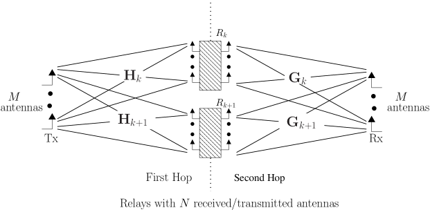
Figure 1: A schematics of a parallel MIMO half-duplexing relay network

III Proposed Method

III-A Cooperative Beamforming Scheme

The equivalent uplink channel can be represented as $\mathbf{H}^{T}=\left[\mathbf{H}_{1}^{T}|\mathbf{H}_{2}^{T}|{\cdots}|\mathbf{H}_{K}^{T}\right]^{T}$. By applying Singular Value Decomposition (SVD) to $\mathbf{H}$, we have $\mathbf{H}=\mathbf{U}\mathbf{\Lambda}^{\frac{1}{2}}\mathbf{V}^{H}$. Therefore, the diagonal matrix $\mathbf{\Lambda}$ has at most $M$ nonzero diagonal entries corresponding to the nonzero singular values of $\mathbf{H}$. Consequently, we can rearrange the SVD such that $\mathbf{U}$ is of size $NK\times{M}$ while $\mathbf{V}$ and $\mathbf{\Lambda}$ are $M\times{M}$ matrices. $\mathbf{U}$ can be partitioned to $M\times{N}$ sub-matrices as $\mathbf{U}=\left[\mathbf{U}_{1}^{T}|\mathbf{U}_{2}^{T}|{\cdots}|\mathbf{U}_{K}^{T}\right]^{T}.$ Suppose the $k$th relay multiplies its received signal by $\mathbf{U}_{k}^{H}$, then passes it through the zero-forcing matrix $\mathbf{G}_{k}^{\dagger}$, and finally amplifies it with a constant scalar $\alpha$ independent of $k$; equivalently, we have $\mathbf{F}_{k}=\alpha\mathbf{G}_{k}^{\dagger}\mathbf{U}_{k}^{H}$. At the receiver side, we have (figure 2)

$$\mathbf{y} = \alpha\sum_{k=1}^{K}{\mathbf{G}_{k}\mathbf{t}_{k}}+\mathbf{z}$$ (4)

$$= \alpha\sum_{k=1}^{K}{\mathbf{G}_{k}\mathbf{G}_{k}^{\dagger}\mathbf{U}_{k}^{H}\mathbf{r}_{k}}+\mathbf{z}$$

$$= \alpha{\mathbf{U}^{H}\mathbf{r}}+\mathbf{z}$$

$$= \alpha\mathbf{U}^{H}\left(\mathbf{H}\mathbf{x}+\mathbf{n}\right)+\mathbf{z}$$

$$= \alpha\left(\mathbf{\Lambda}^{\frac{1}{2}}\mathbf{V}^{H}\mathbf{x}+\mathbf{n}_{u}\right)+\mathbf{z},$$

where $\mathbf{n}=\left[\mathbf{n}_{1}^{T}|\mathbf{n}_{2}^{T}|{\cdots}|\mathbf{n}_{K}^{T}\right]^{T}$ , $\mathbf{r}=\left[\mathbf{r}_{1}^{T}|\mathbf{r}_{2}^{T}|{\cdots}|\mathbf{r}_{K}^{T}\right]^{T}$, and $\mathbf{n}_{u}=\mathbf{U}^{H}\mathbf{n}\sim{\mathcal{CN}(\mathbf{0},\mathbf{I}_{M})}$. If the transmitter beamforms its data vector as $\mathbf{x}=\mathbf{V}\mathbf{x}^{\prime}$, the end-to-end channel becomes

$$\mathbf{y}=\alpha\left(\mathbf{\Lambda}^{\frac{1}{2}}\mathbf{x}^{\prime}+\mathbf{n}_{u}\right)+\mathbf{z}.$$ (5)

Equation (5) shows that the end-to-end channel is diagonal and the noise vector is white Gaussian. Note that the complexity of the decoder in such a channel is linear in terms of the number of transmitter’s antennas, $M$, and also there is no interference among different data streams. In fact, the output signals of the relays not only do not interfere with each other, but also add constructively at the receiver side. Moreover, as it is shown in section IV, for $\alpha\rightarrow\infty$, the achievable rate of such a scheme converges to the point-to-point capacity of the uplink channel which is shown to be an upper-bound on the capacity of the parallel relay system.

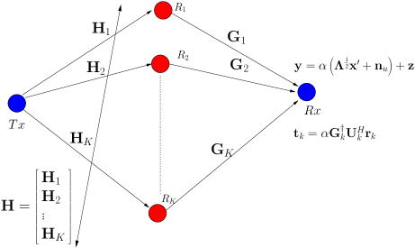
Figure 2: Cooperative Beamforming Scheme

The problem is that the value of $\alpha$ is dominated by

$$\alpha=\sqrt{\frac{P}{\max_{k}{\mathbb{E}_{\mathbf{x},\mathbf{n}_{k}}\left[\left\|\mathbf{G}_{k}^{\dagger}\mathbf{U}_{k}^{H}\mathbf{r}_{k}\right\|^{2}\right]}}}.$$ (6)

This guarantees that the output power of all relays is less than or equal to $P$. However, by applying (6), the value of $\alpha$ could be small in the cases where the downlink channel of any of the relays is ill conditioned. This means that while the output power of the worst relay (according to (6)) is equal to the maximum possible value, i.e. $P$, there may be many relays with the output power far less than $P$. This phenomenon degrades the performance, as in this case the downlink noise, $\mathbf{z}$, would be the dominant noise in (5).

III-B Incremental Cooperative Beamforming Scheme (ICBS)

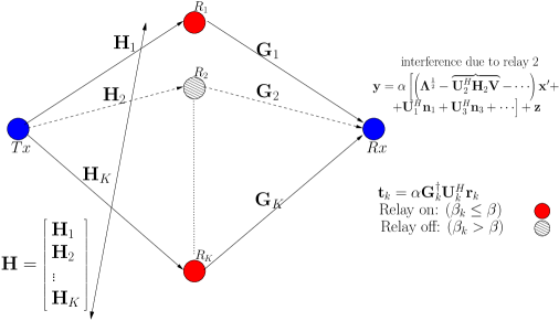
Figure 3: Incremental Cooperative Beamforming Scheme

As the number of relays increases, we expect (as shown in (6)) to have smaller values of $\alpha$ with high probability. In other words, there is a higher chance of having at least one ill-conditioned downlink channel among the relays. In this case, we can select a subset of relays which are in good condition and turn off the rest. In this variant of CBS, we select a subset of relays which results in a high value of $\alpha$. Defining $\beta_{k}\triangleq\mathbb{E}_{\mathbf{x},\mathbf{n}_{k}}\left[\left\|\mathbf{G}_{k}^{\dagger}\mathbf{U}_{k}^{H}\mathbf{r}_{k}\right\|^{2}\right]$, we activate the relays which satisfy $\beta_{k}\leq{\beta}$, where $\beta$ is a predefined threshold. In this manner, it is guaranteed that $\alpha\geq{\sqrt{\frac{P}{\beta}}}$. This improvement in the value of $\alpha$ is realized at the expense of turning off some of the relays, creating interference in the equivalent point-to-point channel. More precisely, by defining $\mathcal{A}=\left\{k|\beta_{k}>\beta\right\}$, we have (figure 3)

$$\mathbf{y}=\alpha\left(\left(\mathbf{\Lambda}^{\frac{1}{2}}-\sum_{k\in\mathcal{A}}{\mathbf{U}_{k}^{H}\mathbf{H}_{k}\mathbf{V}}\right)\mathbf{x}^{\prime}+\sum_{k\in\mathcal{A}^{c}}{\mathbf{U}_{k}^{H}\mathbf{n}_{k}}\right)+\mathbf{z}.$$ (7)

As (7) shows, by decreasing the value of $\beta$, one can guarantee a large value of $\alpha$ while increasing the gap of the equivalent channel matrix to $\mathbf{\Lambda}^{\frac{1}{2}}$. It will be shown in the next section that for large number of relays, it is possible to guarantee both having a large value of $\alpha$ and a small deviation from $\mathbf{\Lambda}^{\frac{1}{2}}$. Moreover, we show that by appropriately choosing the value of $\beta$, the rate of such a scheme would be at most $O\left(\frac{1}{\log\left(K\right)}\right)$ below the corresponding capacity.

III-C A Note on CSI Assumption

In the BNOP scheme, it is assumed that each relay knows its corresponding forward and backward channels, i.e. $\mathbf{H}_{k}$ and $\mathbf{G}_{k}$, and at the receiver side, the effective signal power and the effective interference plus noise power are known for each antenna. However, in CBS and ICBS, it is assumed that the transmitter knows the uplink channel, i.e. $\mathbf{H}_{1},\cdots,\mathbf{H}_{K}$, and sends the $N\times M$ matrix $\mathbf{U}_{k}$ to the $k$’th relay, $k=1,\cdots,K$. This assumption is reasonable when the uplink channel is slow-fading; for example, in the case that the transmitter and all the relay nodes are fixed. Furthermore, similar to the BNOP scheme, we assume that each relay knows its forward channel, i.e. $\mathbf{G}_{k}$. In addition, in CBS, it is assumed that the value of $\alpha$ is set by negotiating between the relays through sending their corresponding $\beta_{k}$ to the transmitter. This assumption is not required in ICBS, as the value of $\alpha$ can be set as $\alpha=\sqrt{\frac{P}{\beta}}$, where $\beta$ is a predefined threshold. Finally, in both CBS and ICBS, it is assumed that the receiver has the perfect knowledge about the equivalent point-to-point channel from the transmitter to the receiver. This information can be obtained through sending pilot signals by the transmitter, amplified and forwarded at the relay nodes in the same manner as the information signal. In CBS, as the equivalent point-to-point channel is diagonal, this assumption is equivalent to knowing the equivalent signal to noise ratio at each antenna.

IV Asymptotic Analysis

In this section, we consider the asymptotic behavior ($K\rightarrow\infty$) of the achievable rate of ICBS. We show that by properly choosing the value of $\beta$, the achievable rate of ICBS converges rapidly to the capacity (the difference approaches zero as $O\left(\frac{1}{\log(K)}\right)$). The sequence of proof is as follows. In Lemma 1, we relate $\mathbb{P}\left[v>\xi\right]$ (the probability that the norm of interference term defined in equation (7) exceeds a certain threshold) to ${\mathbb{P}}[k\in\mathcal{A}]$ (the probability of turning off a relay) and $\mathbb{P}[\|\mathbf{U}_{k}\|^{2}>\gamma]$ (the probability of having a sub-matrix with a large norm in the unitary matrix obtained from the SVD of $\mathbf{H}$). In Lemma 2, we bound $\mathbb{P}[\|\mathbf{U}_{k}\|^{2}>\gamma]$. In Lemma 3, we bound ${\mathbb{P}}[k\in\mathcal{A}]$. As a result, in Lemma 4, we show that by properly choosing the value of $\beta$, with high probability, one can simultaneously reduce the effect of the interference to $o(K)$ and maintain a large value of $\alpha$. In Lemma 5, we show that with high probability, the minimum singular value of $\mathbf{H}$ scales as $O(K)$. Putting Lemmas 4 and 5 together, with high probability, the ratio of the power of interference to the power of signal approaches zero. Finally, in Theorem 1, we prove the main result by showing that the achievable rate of ICBS converges to the capacity of the uplink channel. This is proved using the fact that the capacity of the uplink channel is an upper-bound on the capacity of parallel MIMO relay network. As a consequence stated in corollary 1, the achievable rate of ICBS, the achievable rate of the AF protocol, the point-to-point capacity of the uplink channel, and the capacity of the parallel MIMO relay network are asymptotically equal. As another consequence, the difference of the rates scales as $O(\frac{1}{\log(K)})$.

Using the proof of Lemma 4 and Theorem 1, Theorem 2 shows that as long as the power of relays behaves as $P_{r}(K)=\omega\left(\frac{P}{K}\log^{9}\left(K\right)\right)$, the same rate is achievable by ICBS. Finally, in Theorem 3, we study the asymptotic SNR behavior of CBS and ICBS, and show that, unlike the matched filtering scheme of BNOP, CBS and its variant achieve the full multiplexing gain, regardless of the number of relays.

Lemma 1

Consider a parallel MIMO relay network with $K$ relays using ICBS. We have

$$\mathbb{P}\left[v>\xi\right] \leq \frac{MNK^{2}}{\xi}\left(\mathbb{P}[B_{k}]+\gamma{\mathbb{P}}[A_{k}]\right),$$ (8)

where $v$ is defined as $v=\left\|\sum_{k\in\mathcal{A}}{\mathbf{U}_{k}^{H}\mathbf{H}_{k}}\right\|^{2}$ , and $A_{k}$ and $B_{k}$ are indicator variables defined as $A_{k}\equiv{(k\in\mathcal{A})}$ and $B_{k}\equiv{(\|\mathbf{U}_{k}\|^{2}>\gamma)}$, respectively.

Proof.

Let us define $\mathbf{U}_{\mathcal{A}}=\left[\mathbf{U}_{k}^{T}|k\in\mathcal{A}\right]^{T}$ and $\mathbf{H}_{\mathcal{A}}=\left[\mathbf{H}_{k}^{T}|k\in\mathcal{A}\right]^{T}$. We have

$$\mathbb{P}\left[v>\xi\right] = \mathbb{P}\left[\|\mathbf{U}_{\mathcal{A}}^{H}\mathbf{H}_{\mathcal{A}}\|^{2}>\xi\right]$$ (9)

$$\stackrel{{\scriptstyle(a)}}{{\leq}} \frac{\mathbb{E}\left[\|\mathbf{U}_{\mathcal{A}}^{H}\mathbf{H}_{\mathcal{A}}\|^{2}\right]}{\xi}$$

$$\stackrel{{\scriptstyle(b)}}{{\leq}} \frac{\mathbb{E}\left[\|\mathbf{U}_{\mathcal{A}}\|^{2}\|\mathbf{H}_{\mathcal{A}}\|^{2}\right]}{\xi}$$

$$\stackrel{{\scriptstyle(c)}}{{\leq}} \frac{\mathbb{E}\left[\|\mathbf{U}_{\mathcal{A}}\|^{2}\|\mathbf{H}\|^{2}\right]}{\xi}$$

$$\stackrel{{\scriptstyle(d)}}{{=}} \frac{\mathbb{E}\left[\|\mathbf{U}_{\mathcal{A}}\|^{2}\right]\mathbb{E}\left[\|\mathbf{H}\|^{2}\right]}{\xi}$$

$$= \frac{MNK\mathbb{E}\left[\|\mathbf{U}_{\mathcal{A}}\|^{2}\right]}{\xi}$$

Here, Markov inequality is applied to derive inequality $(a)$. $(b)$ is obtained by applying the norm product inequality on matrices. $(c)$ results from the fact that $\|\mathbf{H}_{\mathcal{A}}\|^{2}\leq\|\mathbf{H}\|^{2}$. Finally, equation $(d)$ follows from the fact that the left unitary matrix, i.e. $\mathbf{U}$, resulted from the SVD of an i.i.d. complex Gaussian matrix, is independent of its singular value matrix, i.e. $\mathbf{\Lambda}^{\frac{1}{2}}$ ,[19], and the fact that $\|\mathbf{H}\|^{2}$ is a function of $\mathbf{\Lambda}$.

To upper-bound $\mathbb{E}\left[\|\mathbf{U}_{\mathcal{A}}\|^{2}\right]$, we have

$$\mathbb{E}\left[\|\mathbf{U}_{\mathcal{A}}\|^{2}\right] = \mathbb{E}\left[\sum_{k=1}^{K}{A_{k}\|\mathbf{U}_{k}\|^{2}}\right]$$ (10)

$$\stackrel{{\scriptstyle(a)}}{{=}} K\mathbb{E}\left[{A}_{k}\|\mathbf{U}_{k}\|^{2}\right]$$

$$= K\mathbb{E}\left[\|\mathbf{U}_{k}\|^{2}|A_{k}\right]\mathbb{P}[A_{k}]$$

$$= K\mathbb{E}\left[\|\mathbf{U}_{k}\|^{2}|A_{k},B_{k}\right]\mathbb{P}[A_{k},B_{k}]$$

$$+ K\mathbb{E}\left[\|\mathbf{U}_{k}\|^{2}|A_{k},B_{k}^{c}\right]\mathbb{P}[A_{k},B_{k}^{c}]$$

$$\stackrel{{\scriptstyle(b)}}{{\leq}} K\left(\mathbb{P}[A_{k},B_{k}]+\gamma\mathbb{P}[A_{k},B_{k}^{c}]\right)$$

$$\stackrel{{\scriptstyle(c)}}{{\leq}} K\left(\mathbb{P}[B_{k}]+\gamma\mathbb{P}[A_{k}]\right),$$

where $(a)$ follows from the fact the channels are symmetric, $(b)$ follows from the fact that the norm of $\mathbf{U}_{k}$ is upper-bounded by 1 and conditioned on the event $B_{k}^{c}$, it is upper-bounded by $\gamma$, and finally $(c)$ follows from the basic probability inequalities. Combining inequalities (9) and (10) completes the proof. ∎

Lemma 2

Consider a $KN\times{M}$ Unitary matrix $\mathbf{U}$, where its columns $\mathbf{U}_{i}$, $i=1,\cdots,M$, are isotropically distributed unit vectors in $\mathbb{C}^{NK\times{1}}$. Let $\mathbf{W}$ be an arbitrary $N\times{M}$ sub-matrix of $\mathbf{U}$. Then, for a predefined value of $M$ and $N$ and assuming $\gamma=\omega\left(\frac{1}{K}\right)$, as $K\to\infty$, we have

$$\mathbb{P}\left[\|\mathbf{W}\|^{2}\geq\gamma\right]=O\left({{\left(K\gamma\right)^{(N-1)}e^{-\frac{\gamma}{M}NK}}}\right)$$ (11)

Proof.

See Appendix A. ∎

Lemma 3

For a small enough value of $\delta$, we have

$$\mathbb{P}[A_{k}]\leq\mathbb{P}[B_{k}]+c_{1}\sqrt{\delta}+c_{2}e^{-\frac{d}{\sqrt{\delta}}},$$ (12)

where $\delta=\frac{\gamma}{\beta}$, and $c_{1},c_{2}$ and $d$ are positive constant parameters independent of $K,\beta$, and $\gamma$.

Proof.

Assume $k$’th relay is off. Hence, we have

$$\beta<\mathbb{E}_{\mathbf{x},\mathbf{n}_{k}}\left[\left\|\mathbf{G}_{k}^{\dagger}\mathbf{U}_{k}^{H}\mathbf{r}_{k}\right\|^{2}\right]\stackrel{{\scriptstyle(a)}}{{\leq}}{\lambda_{\min}^{-1}(\mathbf{G}_{k})}\|\mathbf{U}_{k}\|^{2}\left(1+P\|\mathbf{H}_{k}\|^{2}\right).$$ (13)

Here, $(a)$ follows from the product norm inequality of matrices and independency of the noise from other random variables in the system. Defining the events

$$C_{k} \equiv \left(\lambda_{\min}(\mathbf{G}_{k})<\frac{\|\mathbf{U}_{k}\|^{2}}{\beta}(1+P\|\mathbf{H}_{k}\|^{2})\right),$$ (14)

$$D_{k} \equiv \left(\lambda_{\min}(\mathbf{G}_{k})<\delta\left(1+P\|\mathbf{H}_{k}\|^{2}\right)\right),$$ (15)

we have

$$\mathbb{P}[A_{k}] \stackrel{{\scriptstyle(a)}}{{\leq}} \mathbb{P}[C_{k}]$$ (16)

$$\stackrel{{\scriptstyle}}{{=}} \mathbb{P}[C_{k}\cap{B_{k}}]+\mathbb{P}[C_{k}\cap{B}_{k}^{c}]$$

$$\stackrel{{\scriptstyle(b)}}{{\leq}} \mathbb{P}[{B_{k}}]+\mathbb{P}[C_{k}|{B}_{k}^{c}]\mathbb{P}[{B}_{k}^{c}]$$

$$\stackrel{{\scriptstyle(c)}}{{\leq}} \mathbb{P}[{B_{k}}]+\mathbb{P}[D_{k}|{{B}_{k}^{c}}]\mathbb{P}[{B}_{k}^{c}]$$

$$\stackrel{{\scriptstyle(d)}}{{\leq}} \mathbb{P}[{B_{k}}]+\mathbb{P}[D_{k}],$$

where $(a)$ results from (13), $(b)$ and $(d)$ follow from basic probability inequalities and $(c)$ follows from the fact that conditioned on $\|\mathbf{U}_{k}\|^{2}\leq\gamma$, we have $\frac{\|\mathbf{U}_{k}\|^{2}}{\beta}(1+P\|\mathbf{H}_{k}\|^{2})<\delta\left(1+P\|\mathbf{H}_{k}\|^{2}\right)$, which incurs that $C_{k}\subseteq{D_{k}}$. Defining $\mathbf{W}_{k}$ as the submatrix defined on the first $M$ rows of $\mathbf{G}_{k}$, we have

$$\mathbb{P}[D_{k}] \leq \mathbb{P}\left[\left(\lambda_{\min}(\mathbf{G}_{k})\leq\sqrt{\delta}\right)\bigcup\left(1+P\|\mathbf{H}_{k}\|^{2}\geq\frac{1}{\sqrt{\delta}}\right)\right]$$ (17)

$$\stackrel{{\scriptstyle(a)}}{{\leq}} \mathbb{P}\left[\lambda_{\min}(\mathbf{G}_{k})\leq\sqrt{\delta}\right]+\mathbb{P}\left[1+P\|\mathbf{H}_{k}\|^{2}\geq\frac{1}{\sqrt{\delta}}\right]$$

$$\stackrel{{\scriptstyle(b)}}{{\leq}} \mathbb{P}\left[\lambda_{\min}(\mathbf{W}_{k})\leq\sqrt{\delta}\right]+\mathbb{P}\left[1+P\|\mathbf{H}_{k}\|^{2}\geq\frac{1}{\sqrt{\delta}}\right]$$

$$\stackrel{{\scriptstyle(c)}}{{=}} \int_{x=0}^{\sqrt{\delta}}{Me^{-Mx}dx}+\frac{1}{\Gamma(MN)}\int_{x=\frac{1}{P}\left(\frac{1}{\sqrt{\delta}}-1\right)}^{\infty}{x^{MN-1}e^{-x}dx}$$

$$\leq M\sqrt{\delta}+\left[\sum_{m=0}^{MN-1}{\frac{x^{m}e^{-x}}{m!}}\right]_{x=\frac{1}{P}\left(\frac{1}{\sqrt{\delta}}-1\right)}$$

$$\stackrel{{\scriptstyle(d)}}{{\leq}} M\sqrt{\delta}+MNe^{-\frac{1}{2P}\left(\frac{1}{\sqrt{\delta}}-1\right)}$$

$$= M\sqrt{\delta}+MNe^{\frac{1}{2P}}e^{-\frac{1}{2P\sqrt{\delta}}}$$

Here, $(a)$ results from the union bound, $(b)$ results from the fact that $\lambda_{\min}\left(\mathbf{G}_{k}\right)\geq\lambda_{\min}\left(\mathbf{W}_{k}\right)$ which can be shown easily based on the definition of the singular values of a matrix, $(c)$ results from applying the probability density function of the minimum singular value of square i.i.d. complex Gaussian matrix, derived in [20], and also the fact that $\|\mathbf{H}_{k}\|^{2}$ has Chi-Square distribution with $2MN$ degrees of freedom, and finally, $(d)$ results from the assumption that $\delta$ is small enough such that $\forall{}m,0\leq{m}<MN$, we have $\left(\frac{1}{P}(\frac{1}{\sqrt{\delta}}-1)\right)^{m}<e^{\frac{1}{2P}\left(\frac{1}{\sqrt{\delta}}-1\right)}$. By Combining the results of (16) and (17), we obtain (12) and this completes the proof. ∎

Next, we apply Lemmas 1, 2, and 3 to prove that for large values of $K$, by properly choosing the value of $\beta$, ICBS can simultaneously achieve a large value of $\alpha$ and reduce the interference to $o(K)$, with a high probability.

Lemma 4

By assigning $\beta=\frac{1}{\log(K)}$ and $\gamma=\frac{2\log(K)}{K}$, ICBS simultaneously achieves

$$\alpha=\Omega\left(\sqrt{\log(K)}\right),$$ (18)

$$\mathbb{P}\left[v>\frac{K}{\log^{2}(K)}\right]=O\left(\frac{\log^{4}\left(K\right)}{\sqrt{K}}\right),$$ (19)

where $v$ is defined in Lemma 1.

Proof.

Having $\beta=\frac{1}{\log(K)}$, the value of $\alpha$ would be

$$\alpha=\sqrt{\frac{P}{\max_{k\in\mathcal{A}^{c}}{\beta_{k}}}}\geq\sqrt{\frac{P}{\beta}}=\Omega\left(\sqrt{\log(K)}\right),$$ (20)

and this results in (18). Assuming $\xi=\frac{K}{\log^{2}(K)}$, we have

$$\mathbb{P}\left[v>\xi\right] \stackrel{{\scriptstyle(a)}}{{\leq}} MNK\log^{2}(K)\left(\mathbb{P}[B_{k}]+\frac{2\log(K)}{K}\mathbb{P}[A_{k}]\right)$$

$$\stackrel{{\scriptstyle(b)}}{{\leq}} MNK\log^{2}(K)\left[\mathbb{P}[B_{k}]+\frac{2\log(K)}{K}\left(\mathbb{P}[B_{k}]+c_{1}\sqrt{2\frac{\log^{2}(K)}{K}}+{}\right.\right.$$

$$\left.\left.{}c_{2}e^{-d\sqrt{\frac{K}{2\log^{2}(K)}}}\right)\right]$$

$$\stackrel{{\scriptstyle(c)}}{{\leq}} 2MNK\log^{2}(K)\mathbb{P}[B_{k}]+2MN\sqrt{2}c_{1}\frac{\log^{4}(K)}{\sqrt{K}}+2MNc_{2}\frac{\log^{3}(K)}{K}$$

$$= 2MNK\log^{2}(K)\mathbb{P}[B_{k}]+O\left(\frac{\log^{4}(K)}{\sqrt{K}}\right)$$

$$\stackrel{{\scriptstyle(d)}}{{=}} 2MNK\log^{2}(K)O\left(\left(\log(K)\right)^{(N-1)}e^{-\frac{2{N}}{M}\log(K)}\right)+O\left(\frac{\log^{4}(K)}{\sqrt{K}}\right)$$

$$\stackrel{{\scriptstyle(e)}}{{=}} O\left(\frac{\log^{4}(K)}{\sqrt{K}}\right).$$ (22)

Here, $(a)$ follows from Lemma 1, $(b)$ follows from Lemma 3, $(c)$ follows the assumption that $K$ is large enough such that $2\log(K)<K$ and $d\sqrt{2}\frac{\sqrt{{K}}}{\log(K)}\geq{\log(K)}$ , $(d)$ follows from Lemma 2, and $(e)$ follows from the fact that $\frac{2{N}}{M}\geq 2$, which incurs that

$$K\log^{2}(K)O\left(\left(\log(K)\right)^{(N-1)}e^{-\frac{2{N}}{M}\log(K)}\right)\sim O\left(\frac{\log^{N+1}(K)}{K}\right)\sim o\left(\frac{\log^{4}(K)}{\sqrt{K}}\right).$$

This completes the proof of Lemma 4. ∎

Although with the threshold value stated by Lemma 4, the interference term may tend to infinity in terms of $K$, the signal term tends to infinity more rapidly. In fact, as the following Lemma shows, the singular values of the whole uplink channel matrix behave as $O(K)$ with probability 1, as $K\to\infty$.

Lemma 5

Let $\mathbf{A}$ be an $r\times{s}$ matrix whose entries are i.i.d complex Gaussian random variables with zero mean and unit variance. Assume that $r$ is fixed and $s$ tends to infinity. Then, with probability one $\lambda_{\min}(\mathbf{A})\sim{s},$ or more precisely,

$$\mathbb{P}\left[\lambda_{\min}(\mathbf{A})\sim{s\left(1+O\left(\sqrt[4]{\frac{\log(s)}{s}}\right)\right)}\right]\gtrsim{}1-O\left(\frac{1}{s\sqrt{\log{(s)}}}\right),$$ (23)

where $\lambda_{\min}(\mathbf{A})$ denotes the minimum singular value of $\mathbf{A}\mathbf{A}^{H}$.

Proof.

See Appendix B. ∎

Next, we prove the main theorem of this section.

Theorem 1

By setting the threshold as $\beta=\frac{1}{\log(K)}$, the achievable rate of the proposed ICBS converges to the upper-bound capacity defined for the uplink channel. More precisely,

$$\lim_{K\rightarrow{\infty}}{C_{u}(K)-R_{ICBS}(K)}=0,$$ (24)

where $C_{u}(K)=\frac{1}{2}\mathbb{E}_{\mathbf{H}}\left[\max_{\begin{subarray}{c}\mathbf{Q},\rm{Tr}\{\mathbf{Q}\}\leq P\end{subarray}}\log\left(\left|\mathbf{I}_{KN}+\mathbf{H}\mathbf{Q}\mathbf{H}^{H}\right|\right)\right]$ is the point to point ergodic capacity of the uplink channel and $R_{ICBS}(K)$ is the achievable rate of ICBS.

Proof.

By applying the cut-set bound theorem [21] on the broadcast uplink channel, it can be easily verified [1],[2] that the point-to-point capacity of the uplink channel, $C_{u}(K)$, is an upper-bound on the capacity of the parallel MIMO relay network. Note that the factor $\frac{1}{2}$ in the expression of $C_{u}(K)$ is due to the half-duplex relaying. Define $C_{u^{\star}}(K)=\frac{M}{2}\log\left(1+\frac{KNP}{M}\right)$. We first show that $C_{u^{\star}}(K)$ is an upper-bound for $C_{u}(K)$, and then prove that a lower-bound for $R_{ICBS}(K)$ converges to $C_{u^{\star}}(K)$.

$$C_{u}(K) = \frac{1}{2}\mathbb{E}_{\mathbf{H}}\left[\max_{\begin{subarray}{c}\mathbf{Q}\\ \mbox{Tr}\{\mathbf{Q}\}\leq P\end{subarray}}\log\left(\left|\mathbf{I}_{KN}+\mathbf{H}\mathbf{Q}\mathbf{H}^{H}\right|\right)\right]$$ (25)

$$\stackrel{{\scriptstyle(a)}}{{=}} \frac{1}{2}\mathbb{E}_{\mathbf{H}}\left[\max_{\begin{subarray}{c}\mathbf{Q}\\ \mbox{Tr}\{\mathbf{Q}\}\leq P\end{subarray}}\log\left(\left|\mathbf{I}_{M}+\mathbf{H}^{H}\mathbf{H}\mathbf{Q}\right|\right)\right]$$

$$\stackrel{{\scriptstyle(b)}}{{\leq}} \frac{1}{2}\mathbb{E}_{\mathbf{H}}\left[\max_{\begin{subarray}{c}\mathbf{Q}\\ \mbox{Tr}\{\mathbf{Q}\}\leq P\end{subarray}}M\log\left(1+\frac{\mbox{Tr}\left\{{\mathbf{H}^{H}\mathbf{H}\mathbf{Q}}\right\}}{M}\right)\right]$$

$$\stackrel{{\scriptstyle(c)}}{{\leq}} \frac{M}{2}\mathbb{E}_{\mathbf{H}}\left[\max_{\begin{subarray}{c}\mathbf{Q}\\ \mbox{Tr}\{\mathbf{Q}\}\leq P\end{subarray}}\log\left(1+\frac{\mbox{Tr}\left\{\mathbf{H}^{H}\mathbf{H}\right\}\mbox{Tr}\left\{\mathbf{Q}\right\}}{M}\right)\right]$$

$$\stackrel{{\scriptstyle(d)}}{{\leq}} \frac{M}{2}\log\left(1+\frac{P}{M}\mathbb{E}_{\mathbf{H}}\left[\mbox{Tr}\left\{\mathbf{H}^{H}\mathbf{H}\right\}\right]\right)$$

$$= C_{u^{\star}}(K).$$

Here, $(a)$ follows from the matrix determinant equality , $(b)$ results from the fact that for any positive semidefinite matrix $\mathbf{A}$, we have $|\mathbf{A}|\leq\left(\frac{\mbox{Tr}\left\{\mathbf{A}\right\}}{M}\right)^{M}$, $(c)$ follows from the generalization of the Cauchy-Schwarz inequality to the positive semidefinite matrices, and $(d)$ follows from the concavity of the logarithm function. Rephrasing (7), we have

$$\mathbf{y} = \alpha\mathbf{H}^{\star}\mathbf{x}^{\prime}+\mathbf{n}^{\star},$$ (26)

where

$$\mathbf{H}^{\star} = \mathbf{\Lambda}^{\frac{1}{2}}-\sum_{k\in\mathcal{A}}{\mathbf{U}_{k}^{H}\mathbf{H}_{k}\mathbf{V}},$$ (27)

$$\mathbf{n}^{\star} = \alpha\sum_{k\in\mathcal{A}^{c}}{\mathbf{U}_{k}^{H}\mathbf{n}_{k}}+\mathbf{z}\sim\mathcal{CN}\left(\mathbf{0},\mathbf{P}_{\mathbf{n}^{\star}}\right),$$ (28)

where $\mathbf{P}_{\mathbf{n}^{\star}}=\alpha^{2}\left(\sum_{k\in\mathcal{A}^{c}}{\mathbf{U}_{k}^{H}\mathbf{U}_{k}}\right)+\mathbf{I}_{M}$. The achievable rate of such a system is

$$R_{ICBS}(K) = \frac{1}{2}\mathbb{E}_{\mathbf{H}}\left[\log\left(\left|\mathbf{I}_{M}+\alpha^{2}\frac{P}{M}\mathbf{H}^{\star}\mathbf{H}^{\star{H}}\mathbf{P}_{\mathbf{n}^{\star}}^{-1}\right|\right)\right]$$ (29)

$$\geq \frac{1}{2}\mathbb{E}_{\mathbf{H}}\left[\log\left(\left|\alpha^{2}\frac{P}{M}\mathbf{H}^{\star}\mathbf{H}^{\star{H}}\mathbf{P}_{\mathbf{n}^{\star}}^{-1}\right|\right)\right]$$

$$\stackrel{{\scriptstyle(a)}}{{\geq}} \frac{1}{2}\mathbb{E}_{\mathbf{H}}\left[\log\left(\left|\frac{\alpha^{2}}{1+\alpha^{2}}\frac{P}{M}\mathbf{H}^{\star}\mathbf{H}^{\star{H}}\right|\right)\right]$$

$$= \frac{M}{2}\log\left(\frac{\alpha^{2}}{1+\alpha^{2}}\right)+\frac{1}{2}\mathbb{E}_{\mathbf{H}}\left[\log\left(\left|\frac{P}{M}\mathbf{H}^{\star}\mathbf{H}^{\star{H}}\right|\right)\right],$$

where $(a)$ follows from the fact that $\mathbf{P}_{\mathbf{n}^{\star}}=(\alpha^{2}+1)\mathbf{I}_{M}-\alpha^{2}\left(\sum_{k\in\mathcal{A}}{\mathbf{U}_{k}^{H}\mathbf{U}_{k}}\right)$ which results in $\mathbf{P}_{\mathbf{n}^{\star}}\preccurlyeq(\alpha^{2}+1)\mathbf{I}_{M}$, or equivalently $\mathbf{P}_{\mathbf{n}^{\star}}^{-1}\succcurlyeq\frac{1}{\alpha^{2}+1}\mathbf{I}_{M}$. For convenience, let

$$R_{L}(K)=\frac{1}{2}\mathbb{E}_{\mathbf{H}}\left[\log\left(\left|\frac{P}{M}\mathbf{H}^{\star}\mathbf{H}^{\star{H}}\right|\right)\right].$$

Since $\alpha$ is lower-bounded by the inverse of the threshold as $\alpha\geq\sqrt{\frac{P}{\beta}}$, we have $\lim_{K\rightarrow\infty}{\frac{M}{2}\log\left(\frac{\alpha^{2}}{1+\alpha^{2}}\right)}=0$, or equivalently

$$\lim_{K\rightarrow\infty}R_{ICBS}(K)-R_{L}(K)\geq 0.$$ (30)

Define the events $E_{K}$ and $F_{K}$ as $E_{K}\equiv\left(\lambda_{\min}\left(\mathbf{H}\right)\gtrsim{KN}\left[1+O\left(\sqrt[4]{\frac{\log{K}}{K}}\right)\right]\right)$ and $F_{K}\equiv\left(\left\|\mathbf{U}_{\mathcal{A}}^{H}\mathbf{H}_{\mathcal{A}}\right\|^{2}\leq{\frac{K}{\log^{2}(K)}}\right)$. Consequently, we have

$$\mathbb{P}\left[E_{K},F_{K}\right] \stackrel{{\scriptstyle(a)}}{{\geq}} 1-\mathbb{P}[{E}_{K}^{c}]-\mathbb{P}[{F}_{K}^{c}]$$ (31)

$$\stackrel{{\scriptstyle(b)}}{{\gtrsim}} 1+O\left(\frac{1}{K\sqrt{\log{K}}}\right)+O\left(\frac{\log^{4}(K)}{\sqrt{K}}\right)$$

$$\thicksim 1+O\left(\frac{\log^{4}(K)}{\sqrt{K}}\right).$$

Here, $(a)$ follows from union bound inequality and $(b)$ follows from Lemmas 4 and 5. Assume the diagonal entries of $\mathbf{\Lambda}$ are ordered as $\lambda_{1}(\mathbf{H})\geq\lambda_{2}(\mathbf{H})\geq\cdots\geq\lambda_{M}(\mathbf{H})$. Thus, $R_{L}(K)$ can be lower bounded as

$$R_{L}(K) \geq \frac{1}{2}\mathbb{P}\left[E_{K},F_{K}\right]\mathbb{E}_{\mathbf{H}}\left[\log\left(\left|\frac{P}{M}\mathbf{H}^{\star}\mathbf{H}^{\star{H}}\right|\right)\Bigg{|}E_{K},F_{K}\right]$$

$$= \mathbb{P}\left[E_{K},F_{K}\right]\mathbb{E}_{\mathbf{H}}\left[\log\left(\left|\sqrt{\frac{P}{M}}\left(\mathbf{\Lambda}^{\frac{1}{2}}-\mathbf{U}_{\mathcal{A}}^{H}\mathbf{H}_{\mathcal{A}}\mathbf{V}\right)\right|\right)\Bigg{|}E_{K},F_{K}\right]$$

$$\stackrel{{\scriptstyle(a)}}{{\geq}} \mathbb{P}\left[E_{K},F_{K}\right]\mathbb{E}_{\mathbf{H}}\left[\log\left(\left(\frac{P}{M}\right)^{\frac{M}{2}}\left(\prod_{i=1}^{M}{\lambda_{i}^{\frac{1}{2}}\left(\mathbf{H}\right)}-{}\right.\right.\right.$$

$$\left.\left.\left.{}-\sum_{i=1}^{M}{i!\binom{M}{i}\left\|\mathbf{U}_{\mathcal{A}}^{H}\mathbf{H}_{\mathcal{A}}\mathbf{V}\right\|_{\star}^{i}\prod_{j=1}^{M-i}{\lambda_{j}^{\frac{1}{2}}{\left(\mathbf{H}\right)}}}\right)\right)\Bigg{|}E_{K},F_{K}\right]$$

$$\stackrel{{\scriptstyle(b)}}{{\geq}} \mathbb{P}\left[E_{K},F_{K}\right]\mathbb{E}_{\mathbf{H}}\left[\log\left(\left(\frac{P}{M}\right)^{\frac{M}{2}}\prod_{i=1}^{M}{\lambda_{i}^{\frac{1}{2}}\left(\mathbf{H}\right)}\cdot{}\right.\right.$$

$$\left.\left.{}\cdot\left(1-\sum_{i=1}^{M}{i!\binom{M}{i}\left(\frac{\left\|\mathbf{U}_{\mathcal{A}}^{H}\mathbf{H}_{\mathcal{A}}\right\|^{2}}{\lambda_{\min}\left(\mathbf{H}\right)}\right)^{\frac{i}{2}}}\right)\right)\Bigg{|}E_{K},F_{K}\right]$$

$$\stackrel{{\scriptstyle(c)}}{{\gtrsim}} \mathbb{P}\left[E_{K},F_{K}\right]\mathbb{E}_{\mathbf{H}}\left[\log\left(\left(\frac{P}{M}\right)^{\frac{M}{2}}\prod_{i=1}^{M}{\lambda_{i}^{\frac{1}{2}}\left(\mathbf{H}\right)}\cdot{}\right.\right.$$

$$\left.\left.{}\cdot\left(1-\sum_{i=1}^{M}{i!\binom{M}{i}\left({N\log^{2}(K)\left[1+O\left(\sqrt[4]{\frac{\log{K}}{K}}\right)\right]}\right)^{\frac{-i}{2}}}\right)\right)\Bigg{|}E_{K},F_{K}\right]$$

$$\gtrsim \mathbb{P}\left[E_{K},F_{K}\right]\left\{\frac{M}{2}\log\left(\frac{P}{M}\right)+\frac{1}{2}\sum_{i=1}^{M}{\mathbb{E}_{\mathbf{H}}\left[\log{\left(\lambda_{i}\left(\mathbf{H}\right)\right)}\Big{|}E_{K},F_{K}\right]}\right.-$$

$$\left.{}-\frac{M}{\sqrt{N}\log(K)}\left(1+O\left(\frac{1}{\log(K)}\right)\right)\right\}$$

$$\stackrel{{\scriptstyle(d)}}{{\gtrsim}} \mathbb{P}\left[E_{K},F_{K}\right]\Bigg{\{}\frac{M}{2}\log\left(\frac{P}{M}\right)+\frac{M}{2}\log\left(KN\left[1+O\left(\sqrt[4]{\frac{\log{K}}{K}}\right)\right]\right)-{}$$

$$\left.{}-\frac{M}{\sqrt{N}\log(K)}\left(1+O\left(\frac{1}{\log(K)}\right)\right)\right\}$$

$$\stackrel{{\scriptstyle(e)}}{{\gtrsim}} \left\{\frac{M}{2}\log\left(\frac{KNP}{M}\right)+O\left(\frac{1}{\log(K)}\right)\right\}\mathbb{P}\left[E_{K},F_{K}\right]$$

$$\stackrel{{\scriptstyle(f)}}{{\gtrsim}} \left\{\frac{M}{2}\log\left(\frac{KNP}{M}\right)+O\left(\frac{1}{\log(K)}\right)\right\}\left[1+O\left(\frac{\log^{4}(K)}{\sqrt{K}}\right)\right]$$

$$\stackrel{{\scriptstyle(g)}}{{\sim}} \frac{M}{2}\log\left(\frac{KNP}{M}\right)+O\left(\frac{1}{\log(K)}\right).$$ (34)

Here, $(a)$ follows from an upper-bound on the determinant expansion of $\mathbf{\Lambda}^{\frac{1}{2}}-\mathbf{U}_{\mathcal{A}}^{H}\mathbf{H}_{\mathcal{A}}\mathbf{V}$, expanded over all possible set entries between $\mathbf{\Lambda}$ and $\mathbf{U}_{\mathcal{A}}^{H}\mathbf{H}_{\mathcal{A}}\mathbf{V}$, $(b)$ follows from the fact that the Frobenius norm of a matrix is an upper-bound on the square of the maximum absolute value among its entries and also $\forall{i}:\lambda_{i}(\mathbf{H})\geq\lambda_{\min}(\mathbf{H})$, $(c)$ follows from the fact that the expectation is derived conditioned on the events $E_{K}$ and $F_{K}$, $(d)$ holds due to the fact that conditioned on $E_{K}$, we have $\lambda_{i}\left(\mathbf{H}\right)\gtrsim{KN}\left[1+O\left(\sqrt[4]{\frac{\log{K}}{K}}\right)\right]$, $(e)$ follows from the fact that $\log\left(1+O\left(\sqrt[4]{\frac{\log(K)}{K}}\right)\right)\sim O\left(\sqrt[4]{\frac{\log(K)}{K}}\right)\sim o\left(\frac{1}{\log^{2}(K)}\right)$, $(f)$ results from (31), and finally, $(g)$ follows from the fact that $O\left(\frac{\log^{4}(K)}{\sqrt{K}}\right)\sim o\left(\frac{1}{\log(K)}\right)$. Now, defining $R_{S}\left(K\right)=\frac{M}{2}\log\left(\frac{KNP}{M}\right)$, according to (30) and (34), we have

$$\lim_{K\rightarrow\infty}{R_{ICBS}(K)-R_{S}(K)}\geq{0}.$$ (35)

Furthermore, we have:

$$\lim_{K\rightarrow\infty}{C_{u^{\star}}(K)-R_{S}(K)}={0}.$$ (36)

Comparing (25), (35) and (36), and observing the fact that $C_{u}(K)\geq{C}_{ICBS}(K)$, results in (24) and this completes the proof. ∎

Corrolary 1

The capacity of parallel MIMO Relay network, the point-to-point capacity of the cut-set defined on the uplink channel, the achievable rate of amplify and forward relaying, and the achievable rate of ICBS, all converge to $\frac{M}{2}\log\left(\frac{KNP}{M}\right)$, as $K\to\infty$.

Proof.

Defining $C(K)$, $C_{u}(K)$, $R_{AF}(K)$, and $R_{ICBS}(K)$ as the capacity of parallel MIMO Relay network, the point-to-point capacity of the cut-set defined on the uplink channel, the achievable rate of the amplify and forward relaying, and the achievable rate of ICBS, respectively, it is clear that

$$R_{ICBS}(K){\leq}R_{AF}(K){\leq}C(K){\leq}C_{u}(K).$$ (37)

Relying on Theorem 1, we know

$$\lim_{K\rightarrow{\infty}}{C_{u}(K)-R_{S}(K)}=\lim_{K\rightarrow{\infty}}{R_{ICBS}(K)-R_{S}(K)}=0.$$ (38)

By observing that $R_{AF}(K)$ and $C(K)$ are sandwiched between $R_{ICBS}(K)$ and $C_{u}(K)$, Sandwich theorem tells us that

$$\lim_{K\rightarrow{\infty}}{R_{AF}(K)-R_{S}(K)}=\lim_{K\rightarrow{\infty}}{C(K)-R_{S}(K)}=0.$$ (39)

∎

Corrolary 2

Achievable rate of ICBS is at most $O\left(\frac{1}{\log\left(K\right)}\right)$ below the upper-bound corresponding to the cut-set defined on the point-to-point uplink channel, i.e. $C_{u}(K)$.

Proof.

Following the proof of Theorem 1, we observe

$$C_{u}(K)-R_{ICBS}(K)\leq{\Delta}R_{1}+{\Delta}R_{2}+{\Delta}R_{3},$$ (40)

where ${\Delta}R_{1}=\frac{M}{2}\log\left(1+\frac{1}{\alpha^{2}}\right)$ results from the approximation of the first term in (29), ${\Delta}R_{2}=O\left(\frac{1}{\log(K)}\right)$ in (34), and finally, $\Delta{R_{3}}=\frac{M}{2}\log\left(1+\frac{M}{KNP}\right)\sim O\left(\frac{1}{K}\right)$ is the difference between $C_{u^{*}}(K)$ and $R_{S}(K)$. We know that $\alpha\geq\sqrt{\frac{P}{\beta}}=\sqrt{P\log(K)}$, and as a result, ${\Delta}R_{1}=\frac{M}{2}\log\left(1+\frac{1}{P\log(K)}\right)\sim O\left(\frac{1}{\log(K)}\right)$. Comparing the values of $\Delta{R_{i}},1\leq{i}\leq{3}$, we conclude that $C_{u}(K)-R_{ICBS}(K)=O\left(\frac{1}{\log\left(K\right)}\right)$. ∎

Apart from increasing the rate, using parallel relays also increases the reliability of the transmission. As the following corollary shows, the probability of outage when sending information at the rate $O\left(\frac{1}{\log\left(K\right)}\right)$ below the ergodic capacity approaches zero, as $K\to\infty$.

Corrolary 3

Consider the parallel MIMO relay network and ICBS with the threshold value $\beta=\frac{1}{\log\left(K\right)}$. We have

$$\mathbb{P}\left[\frac{1}{2}\log\left(\left|\mathbf{I}_{M}+\alpha^{2}\frac{P}{M}\mathbf{H}^{\star}\mathbf{H}^{\star{H}}\mathbf{P}_{\mathbf{n}^{\star}}^{-1}\right|\right)\lesssim{}C_{u}(K)+O\left(\frac{1}{\log\left(K\right)}\right)\right]\sim{}O\left(\frac{\log^{4}\left(K\right)}{\sqrt{K}}\right).$$

Proof.

Following the proof of Theorem 1, we observe this outage event is a subset of $E_{K}^{c}\bigcup F_{K}^{c}$, whose probability is shown to be $O\left(\frac{\log^{4}\left(K\right)}{\sqrt{K}}\right)$. ∎

Another interesting result is that by increasing the number of relays, each relay can operate with a much lower power as compared to the transmitter, while the scheme achieves the optimum rate. This shows another benefit of using many parallel relays in the network.

Theorem 2

Up to the point that $P_{r}(K)=\omega\left(\frac{P}{K}\log^{9}\left(K\right)\right)$, the achievable rate of ICBS satisfies

$$\lim_{K\rightarrow\infty}{R_{ICBS}(K)-C_{u}(K)}=\lim_{K\rightarrow\infty}R_{ICBS}(K)-\frac{M}{2}\log\left(\frac{KNP}{M}\right)=0.$$ (41)

Proof.

We use the same steps as the proof of Lemma 4 with the same values of $\gamma$ and $\xi$. Rewriting (IV), we have

$$\mathbb{P}[v>\xi]\leq MNK\log^{2}(K)\left[\mathbb{P}[B_{k}]+\frac{2\log(K)}{K}\left(\mathbb{P}[B_{k}]+c_{1}\sqrt{\delta}+c_{2}e^{-\frac{d}{\sqrt{\delta}}}\right)\right],$$ (42)

where $\delta=\frac{\gamma}{\beta}$. In order that the second term in (IV) (or equivalently $\Delta R_{2}$ in (40)) approaches zero, we must have $\mathbb{P}[E_{K},F_{K}]\sim 1+o\left(\frac{1}{\log(K)}\right)$, which implies that $\mathbb{P}[v>\xi]\sim 1+o\left(\frac{1}{\log(K)}\right)$. From the above equation, it follows that having $\beta\sim\omega\left(\frac{\log^{9}(K)}{K}\right)$ incurs that $\sqrt{\delta}=\sqrt{\frac{\gamma}{\beta}}\sim o\left(\sqrt{\frac{\frac{2\log(K)}{K}}{\frac{\log^{9}(K)}{K}}}\right)$, or equivalently, $\sqrt{\delta}\log^{3}(K)\sim o\left(\frac{1}{\log(K)}\right)$, which results in $\mathbb{P}[v>\xi]\sim 1+o\left(\frac{1}{\log(K)}\right)$. Moreover, the first term in (29) (or equivalently $\Delta R_{1}$ in (40)) approaches zero, if $P_{r}(K)=\omega(\beta)$ (or equivalently, $\alpha\sim\omega(1)$). Therefore, having $P_{r}(K)\sim\omega\left(\frac{\log^{9}(K)}{K}\right)$, results in $\Delta R_{1},\Delta R_{2}\to 0$, which implies that $\lim_{K\to\infty}C_{u}(K)-R_{ICBS}(K)=0$. ∎

Theorem 3

The proposed Cooperative Beamforming scheme and its variant achieve the maximum multiplexing gain of the relay channel. More precisely:

$$\lim_{P\rightarrow\infty}{\frac{R_{CBS}(P)}{\log(P)}}=\frac{M}{2},$$ (43)

and $\frac{M}{2}$ is the maximum achievable multiplexing gain of the underlying half duplex system. (Here $R_{CBS}(P)$ is the achievable rate of the proposed scheme for the given power constraint $P$.)

Proof.

We prove the theorem for CBS. The statements of the proof are also valid for the variant of CBS. First of all, from the last theorem, we have

$$C_{u}(P)\leq{C_{u^{\star}}(P)}\stackrel{{\scriptstyle(a)}}{{\leq}}\frac{M}{2}\log\left(\frac{2KNP}{M}\right)=\frac{M}{2}\log\left(\frac{KN}{M}\right)+\frac{M}{2}\log(P)+\frac{M}{2}.$$ (44)

Here, $(a)$ follows from the assumption that $P$ is large enough such that we have $P\geq\frac{M}{KN}$. Thus, the maximum achievable multiplexing gain is

$$r_{\max}=\lim_{P\rightarrow\infty}{\frac{C_{u}(P)}{\log(P)}}\leq\frac{M}{2}.$$ (45)

To prove the theorem, it is sufficient to show that the multiplexing gain of CBS is lower bounded by $\frac{M}{2}$. To show this, we lower-bound the achievable rate of the scheme as follows:

$$R_{CBS}(P) = \frac{1}{2}\mathbb{E}_{\mathbf{G},\mathbf{H}}\left[\log\left(\left|\mathbf{I}_{M}+\frac{\alpha^{2}}{1+\alpha^{2}}\frac{P}{M}\mathbf{\Lambda}\right|\right)\right]$$ (46)

$$\geq \frac{1}{2}\mathbb{E}_{\mathbf{G},\mathbf{H}}\left[\log\left(\left|\frac{\alpha^{2}}{1+\alpha^{2}}\frac{P}{M}\mathbf{\Lambda}\right|\right)\right]$$

$$\geq \frac{M}{2}\log(P)+\frac{M}{2}\mathbb{E}_{\mathbf{H}}\left[\log\left(\lambda_{\min}\left(\mathbf{H}\right)\right)\right]-\frac{M}{2}\log(M)-\frac{M}{2}\mathbb{E}_{\mathbf{G},\mathbf{H}}\left[\log\left(1+\frac{1}{\alpha^{2}}\right)\right]$$

$$\stackrel{{\scriptstyle(a)}}{{\geq}} \frac{M}{2}\log(P)+\frac{M^{2}}{2}\int_{x=0}^{1}e^{-x}\log(x)dx-\frac{M}{2}\log(M)-\frac{M}{2}\mathbb{E}_{\mathbf{G},\mathbf{H}}\left[\log\left(1+\frac{1}{\alpha^{2}}\right)\right]$$

$$\geq \frac{M}{2}\log(P)-\frac{M^{2}}{2}-\frac{M}{2}\log(M)-\frac{M}{2}\mathbb{E}_{\mathbf{G},\mathbf{H}}\left[\log\left(1+\frac{1}{\alpha^{2}}\right)\right],$$

where $(a)$ follows from the fact that $\lambda_{\min}(\mathbf{H})\geq\lambda_{\min}(\mathbf{W})$, where $\mathbf{W}$ is an arbitrary $M\times M$ submatrix of $\mathbf{H}$, noting that $f_{\lambda_{\min}(\mathbf{W})}(\lambda)=Me^{-M\lambda}$, $\lambda>0$. Now, defining $x_{\alpha}=\mathbb{E}_{\mathbf{G},\mathbf{H}}\left[\log\left(1+\frac{1}{\alpha^{2}}\right)\right]$, it is sufficient to show that $x_{\alpha}$ can be upper bounded by a finite expression independent of $P$. Defining $x_{\alpha,k}=\log{\left[1+\lambda_{\min}^{-1}\left(\mathbf{G}_{k}\right)\left(\left\|\mathbf{H}_{k}\right\|^{2}+\frac{1}{P}\right)\right]}$, we have

$$x_{\alpha} = \mathbb{E}_{\mathbf{G},\mathbf{H}}\left[\log\left(1+\frac{\max_{1\leq{k}\leq{K}}{\mathbb{E}_{\mathbf{x},\mathbf{n}_{k}}\left[\left\|\mathbf{G}_{k}^{\dagger}\mathbf{U}_{k}^{H}\mathbf{r}_{k}\right\|^{2}\right]}}{P}\right)\right]$$ (47)

$$= \mathbb{E}_{\mathbf{G},\mathbf{H}}\left[\max_{1\leq{k}\leq{K}}{\log\left(1+\frac{\mathbb{E}_{\mathbf{x},\mathbf{n}_{k}}\left[\left\|\mathbf{G}_{k}^{\dagger}\mathbf{U}_{k}^{H}\mathbf{r}_{k}\right\|^{2}\right]}{P}\right)}\right]$$

$$\stackrel{{\scriptstyle(a)}}{{\leq}} \mathbb{E}_{\mathbf{G},\mathbf{H}}\left[\max_{1\leq{k}\leq{K}}{\log\left(1+\lambda_{\min}^{-1}\left(\mathbf{G}_{k}\right)\left(\left\|\mathbf{H}_{k}\right\|^{2}+\frac{1}{P}\right)\right)}\right]$$

$$= \mathbb{E}_{\mathbf{G},\mathbf{H}}\left[\max_{1\leq{k}\leq{K}}{x_{\alpha,k}}\right]$$

$$\stackrel{{\scriptstyle(b)}}{{\leq}} \mathbb{E}_{\mathbf{G},\mathbf{H}}\left[\sum_{k=1}^{K}{x_{\alpha,k}}\right]$$

$$= K\mathbb{E}_{\mathbf{G},\mathbf{H}}\left[{x_{\alpha,k}}\right]$$

Here, $(a)$ results from matrix product norm inequality and independency of $\mathbf{n}_{k}$ from $\mathbf{H}_{k}$ and $\mathbf{x}$, and $(b)$ follows from the fact that $x_{\alpha,k}$’s are nonnegative i.i.d. random variables. Without loss of generality, we can assume $P$ is large enough such that $P\geq{1}$. We can upper-bound $\mathbb{E}\left[x_{\alpha,k}\right]$ as

$$\mathbb{E}\left[x_{\alpha,k}\right] = \mathbb{E}_{\mathbf{G}_{k},\mathbf{H}_{k}}\left\{\log{\left[1+\lambda_{\min}^{-1}\left(\mathbf{G}_{k}\right)\left(\left\|\mathbf{H}_{k}\right\|^{2}+\frac{1}{P}\right)\right]}\right\}$$ (48)

$$\stackrel{{\scriptstyle(a)}}{{\leq}} \mathbb{E}_{\mathbf{G}_{k},\mathbf{H}_{k}}\left[\log{\left(1+\lambda_{\min}{\left(\mathbf{G}_{k}\right)}+\left\|\mathbf{H}_{k}\right\|^{2}\right)}\right]-\mathbb{E}_{\mathbf{G}_{k}}\left[\log{\left(\lambda_{\min}\left(\mathbf{G}_{k}\right)\right)}\right]$$

$$\stackrel{{\scriptstyle(b)}}{{\leq}} \mathbb{E}_{\mathbf{G}_{k}}\left[\lambda_{\min}{\left(\mathbf{G}_{k}\right)}\right]+\mathbb{E}_{\mathbf{H}_{k}}\left[\left\|\mathbf{H}_{k}\right\|^{2}\right]-\mathbb{E}_{\mathbf{G}_{k}}\left[\log{\left(\lambda_{\min}\left(\mathbf{G}_{k}\right)\right)}\right]$$

$$\stackrel{{\scriptstyle(c)}}{{\leq}} N+MN-M\int_{x=0}^{1}{e^{-Mx}\log(x)dx}$$

$$\leq MN+M+N.$$

Here, $(a)$ follows from the assumption that $P\geq{1}$, $(b)$ follows from the fact that $\log(1+x)\leq{x}$, and $(c)$ follows from the fact that $\mathbb{E}\left[\lambda_{\min}{\left(\mathbf{G}_{k}\right)}\right]\leq\mathbb{E}\left[\frac{\|\mathbf{G}_{k}\|^{2}}{M}\right]=N$, and also $(a)$ in (46). Comparing (46), (47), and (48), we have

$$R_{CBS}\left(P\right)\geq\frac{M}{2}\log(P)+O(1).$$ (49)

As a result

$$r_{CBS}=\lim_{P\rightarrow\infty}{\frac{C_{u}(P)}{\log(P)}}\geq\frac{M}{2}.$$ (50)

Comparing (45) and (50) completes the proof. ∎

Remark - It is claimed in [1] that the proposed BNOP scheme achieves the full multiplexing gain of $\frac{M}{2}$, for $K\to\infty$. However, it should be mentioned that this result is not valid for the asymptotically large values of SNR, for any fixed number of relays. Moreover, it can easily be shown that the interference term increases linearly with SNR, and as a result, the SINR term is limited by a constant value for large SNR values. Therefore, the multiplexing gain of BNOP scheme is zero for any fixed number of relays.

V Simulation Results

Figure 4 shows the simulation results for the achievable rate of ICBS, BNOP matched filtering scheme [1], and the upper-bound of the capacity based on the uplink Cut-Set for varying number of relays. The number of transmitting and receiving antennas in the relays, the transmitter, and the receiver is $M=N=2$, and the SNR is $P_{s}=P_{r}=10dB$. While both of the schemes demonstrate logarithmic scaling of rate in terms of $K$, we observe that there is a significant gap between the BNOP scheme and our scheme, reflecting the gap of $O(1)$ in the achievable rate of [1]. On the other hand, the gap between ICBS and the upper-bound rapidly approaches zero due to the term $O\left(\frac{1}{\log\left(K\right)}\right)$ predicted in Corollary 2.

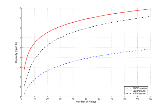
Figure 4: Upper-bound of the capacity, ICBS, and BNOP matched filtering Scheme vs. number of relays in parallel MIMO relay network

VI Conclusion

A simple new scheme, Cooperative Beamforming Scheme (CBS), based on Amplify and Forward (AF) strategy is introduced in a parallel MIMO relay network. A variant of CBS, called Incremental Cooperative Beamforming Scheme (ICBS) is shown to achieve the capacity of parallel MIMO relay network for $K\to\infty$. The scheme is shown to rapidly approach the upper-bound of the capacity with a gap no more than $O\left(\frac{1}{\log\left(K\right)}\right)$. As a result, it is shown that the capacity of a parallel MIMO relay network is $C(K)=\frac{M}{2}\log\left(1+\frac{KNP}{M}\right)+O\left(\frac{1}{\log\left(K\right)}\right)$ in terms of the number of relays, $K$. Moreover, it is shown that as the number of relays increases, the relays in ICBS can operate using much less power without any performance degradation. Finally, the proposed scheme is shown to achieve the maximum multiplexing gain regardless of the number of relays. The simulation results confirm the validity of the theoretical arguments.

Appendix A

Proof of Lemma 2

Let us denote $\mathbf{W}_{i}$ as the $i$th column of $\mathbf{W}$. In [23], it has been shown that

$$f_{\|\mathbf{W}_{i}\|^{2}}(x)=\frac{\Gamma(NK)}{\Gamma(N)\Gamma(NK-N)}x^{N-1}(1-x)^{NK-N-1},\quad i=1,\cdots,M,$$ (51)

which corresponds to the Beta distribution with parameters $N$ and $NK-N$. Therefore, we have

$$\mathbb{P}\left[\|\mathbf{W}\|^{2}\geq\gamma\right] = \mathbb{P}\left[\sum_{i=1}^{M}\|\mathbf{W}_{i}\|^{2}\geq\gamma\right]$$ (52)

$$\leq \mathbb{P}\left[\max_{i}\|\mathbf{W}_{i}\|^{2}\geq\frac{\gamma}{M}\right]$$

$$= \mathbb{P}\left[\bigcup_{i=1}^{M}\mathcal{F}_{i}\right]$$

$$\stackrel{{\scriptstyle(a)}}{{\leq}} M\mathbb{P}\left[\mathcal{F}_{i}\right],$$

where $(a)$ results from the Union bound on the probability, and $\mathcal{F}_{i}\equiv\|\mathbf{W}_{i}\|^{2}\geq\frac{\gamma}{M}$. Defining $\gamma^{\prime}\triangleq\frac{\gamma}{M}$, and using (51), we obtain

$$\mathbb{P}\left[\|\mathbf{W}\|^{2}\geq\gamma\right] \leq M\left(1-F_{\|\mathbf{W}_{i}\|^{2}}(\gamma^{\prime})\right)$$ (53)

$$= M\frac{\Gamma(NK)}{\Gamma(N)\Gamma(NK-N)}\int_{\gamma^{\prime}}^{1}x^{N-1}(1-x)^{NK-N-1}dx$$

$$\stackrel{{\scriptstyle(a)}}{{=}} M\frac{\Gamma(NK)}{\Gamma(N)\Gamma(NK-N)}\left(\frac{\gamma^{\prime(N-1)}(1-\gamma^{\prime})^{NK-N}}{NK-N}\right.+$$

$$\left.\frac{1}{NK-N}\sum_{n=1}^{N-1}\left[\prod_{j=1}^{n}\frac{(N-j)}{(NK-N+j)}\right]\gamma^{\prime(N-n-1)}(1-\gamma^{\prime})^{NK-N+n}\right)$$

$$= M\sum_{n=1}^{N}\frac{(NK-1)!}{(N-n)!(NK-N+n-1)!}\gamma^{\prime N-n}(1-\gamma^{\prime})^{NK-N+n-1}$$

$$\leq M\sum_{n=1}^{N}\frac{(NK\gamma^{\prime})^{N-n}(1-\gamma)^{NK-N}}{(N-n)!}$$

$$\stackrel{{\scriptstyle(b)}}{{\sim}} \frac{M(NK\gamma^{\prime})^{N-1}(1-\gamma^{\prime})^{NK-N}}{(N-1)!}\left[1+O\left(\frac{1}{K\gamma^{\prime}}\right)\right]$$

$$\sim O\left((K\gamma)^{N-1}e^{-\frac{\gamma}{M}NK}\right),$$

where $(a)$ follows from the integration by part, and $(b)$ follows from the fact that $K\gamma^{\prime}\sim\omega(1)$.

$\blacksquare$

Appendix B

Proof of Lemma 5

The $(i,j)$th entry of $\mathbf{A}\mathbf{A}^{H}$, denoted as $[\mathbf{AA}^{H}]_{i,j}$, can be written as

$$[\mathbf{AA}^{H}]_{i,j}=\mathbf{a}_{i}\mathbf{a}_{j}^{H},$$ (54)

where $\mathbf{a}_{i}$ is the vector representing the $i$th row of $\mathbf{AA}^{H}$. Let us define $\mathbf{B}$ as

$$\mathbf{B}\triangleq[\mathbf{b}_{1}^{T}|\cdots|\mathbf{b}_{r}^{T}]^{T},$$ (55)

where $\mathbf{b}_{i}=\dfrac{\mathbf{a}_{i}}{\|\mathbf{a}_{i}\|}$, $i=1,\cdots,r$. We have

$$[\mathbf{BB}^{H}]_{i,j}=\left[\begin{tabular}[]{lc}$1$&$i=j$\\ $\gamma(i,j)$&$i\neq j$\end{tabular}\right.,$$ (58)

where $\gamma(i,j)\triangleq\mathbf{b}_{i}\mathbf{b}_{j}^{H}=\dfrac{\mathbf{a}_{i}\mathbf{a}_{j}^{H}}{\|\mathbf{a}_{i}\|\|\mathbf{a}_{j}\|}$. The pdf of $z(i,j)=|\gamma(i,j)|^{2}$ has been computed in [23], Lemma 3, as

$$p_{z(i,j)}(z)=(s-1)(1-z)^{s-2}.$$ (59)

Let us define $\mathcal{C}$ as the event that $z(i,j)<\frac{1}{\sqrt{s}}$ for all $i\neq j$. Using (59), we have

$$\mathbb{P}[\mathcal{C}] = \mathbb{P}\left[\bigcap_{i\neq j}\left(z(i,j)<\frac{1}{\sqrt{s}}\right)\right]$$ (60)

$$\stackrel{{\scriptstyle(a)}}{{\geq}} 1-\frac{r(r-1)}{2}\left(1-\frac{1}{\sqrt{s}}\right)^{s-1}$$

$$\sim 1+O(e^{-\sqrt{s}}),$$

where $(a)$ results from the Union bound on the probability, noting that $z(i,j)=z(j,i)$, $\forall i,j$. Conditioned on $\mathcal{C}$, the orthogonality defect of $\mathbf{B}$, defined as $\frac{\prod_{i=1}^{r}\|\mathbf{b}_{i}\|^{2}}{\left|\mathbf{BB}^{H}\right|}$, can be written as

$$\delta_{\mathcal{C}}(\mathbf{B}) = \frac{1}{\left|\mathbf{BB}^{H}\right|}$$ (61)

$$= \frac{1}{1+O(\frac{1}{\sqrt{s}})}$$

$$= 1+O\Big{(}\frac{1}{\sqrt{s}}\Big{)},$$

where $\delta_{\mathcal{C}}(\mathbf{B})$ denotes the orthogonality defect of $\mathbf{B}$, conditioned on $\mathcal{C}$. Hence, using the fact that the orthogonality defect of $\mathbf{A}$ and $\mathbf{B}$ are equal, conditioned on $\mathcal{C}$ we can write

$$\prod_{i=1}^{r}\lambda_{i}(\mathbf{A}) = \left|\mathbf{AA}^{H}\right|$$ (62)

$$= \prod_{i=1}^{r}\|\mathbf{a}_{i}\|^{2}\left[1+O\Big{(}\frac{1}{\sqrt{s}}\Big{)}\right],$$

where $\lambda_{i}(\mathbf{A})$’s denote the singular values of $\mathbf{AA}^{H}$. Moreover,

$$\sum_{i=1}^{r}\lambda_{i}(\mathbf{A}) = \mbox{Tr}\{\mathbf{AA}^{H}\}$$ (63)

$$= \sum_{i=1}^{r}\|\mathbf{a}_{i}\|^{2}.$$

Now, let us define events $\mathcal{D}_{i}$ as follows:

$$\mathcal{D}_{i}\equiv\left\{s(1-\epsilon)<\|\mathbf{a}_{i}\|^{2}<s(1+\epsilon)\right\},\quad i=1,\cdots,r,$$ (64)

where $\epsilon\triangleq\sqrt{\frac{2\log(s)}{s}}$. Since $\|\mathbf{a}_{i}\|=\sum_{j=1}^{s}|a_{i,j}|^{2}$, where $a_{i,j}$ denotes the $(i,j)$th entry of $\mathbf{A}$, and having the fact that $|a_{i,j}|^{2}$ are i.i.d. random variables with unit mean and unit variance, using Central Limit Theorem (CLT), $\frac{1}{s}\|\mathbf{a}_{i}\|^{2}$ approaches, in probability, to a Gaussian distribution with unit mean and variance $\frac{1}{s}$, as $s$ tends to infinity. More precisely, defining $X\triangleq\frac{\frac{1}{s}\|\mathbf{a}_{i}\|^{2}}{\sqrt{\frac{1}{s}}}$ and using Theorem 5.24 in [24], we have

$$\mathbb{P}\left[-\sqrt{2\log(s)}<X<\sqrt{2\log(s)}\right] = 1-\left[1-\Phi\left(\sqrt{2\log(s)}\right)\right]\exp\left\{\frac{\gamma_{3}\sqrt{2}\sqrt{\log^{3}(s)}}{3\sigma^{3}\sqrt{s}}\right\}-$$

$${}-\Phi\left(-\sqrt{2\log(s)}\right)\exp\left\{-\frac{\gamma_{3}\sqrt{2}\sqrt{\log^{3}(s)}}{3\sigma^{3}\sqrt{s}}\right\}+$$

$${}+O\left(s^{-1/2}e^{-\log(s)}\right)$$

$$\stackrel{{\scriptstyle(a)}}{{\approx}} 1-\frac{1}{s\sqrt{\pi\log(s)}}\left[1+O\left(\sqrt{\frac{\log^{3}(s)}{s}}\right)\right]+O\left(\frac{1}{s\sqrt{s}}\right),$$

where $\Phi(.)$ denotes the CDF of the normal distribution, and $\sigma^{2}$ and $\gamma_{3}$ denote the second and third moments of $|a_{i,j}|^{2}$, respectively. $(a)$ follows from the approximation of $\Phi(x)$ for large $x$ by $1-\frac{1}{\sqrt{2\pi}x}e^{-\frac{x^{2}}{2}}$ and the fact that $\sigma\sim\gamma_{3}\sim\Theta(1)$. From the above equation, $\mathbb{P}[\mathcal{D}_{i}]$ can be computed as

$$\mathbb{P}[\mathcal{D}_{i}] = \mathbb{P}\left[1-\epsilon<\frac{1}{s}\|\mathbf{a}_{i}\|^{2}<1+\epsilon\right]$$ (66)

$$\sim 1+O\left(\frac{1}{s\sqrt{\log(s)}}\right),$$

in which we have used the definition of $\epsilon$ which is $\sqrt{\frac{2\log(s)}{s}}$. Conditioned on $\mathcal{C}$ and $\mathcal{D}$, where $\mathcal{D}\triangleq\bigcap_{i=1}^{r}\mathcal{D}_{i}$, and using (62) and (63), we can write

$$\eta \triangleq \frac{\prod_{i=1}^{r}\lambda_{i}}{\overline{\lambda}^{r}}$$ (67)

$$= \frac{\prod_{i=1}^{r}\left[s(1+O(\epsilon))\right]\left[1+O\Big{(}\frac{1}{\sqrt{s}}\Big{)}\right]}{\left[\frac{1}{r}\sum_{i=1}^{r}s(1+O(\epsilon))\right]^{r}}$$

$$= 1+O(\epsilon)$$

$$= 1+O\Big{(}\sqrt{\frac{\log(s)}{s}}\Big{)},$$

where $\overline{\lambda}\triangleq\frac{1}{r}\sum_{i=1}^{r}\lambda_{i}$. Suppose that $\lambda_{\min}=\alpha\overline{\lambda}$ ($\alpha<1$). We have

$$\eta \stackrel{{\scriptstyle(a)}}{{\leq}} \frac{\alpha\overline{\lambda}\left[\frac{1}{r-1}(r\overline{\lambda}-\alpha\overline{\lambda})\right]^{r-1}}{\overline{\lambda}^{r}}$$ (68)

$$= \frac{\alpha(r-\alpha)^{r-1}}{(r-1)^{r-1}},$$

where $(a)$ follows from the fact that knowing $\lambda_{\min}$, the product of the rest of the singular values is maximized when they are all equal. Hence, having the sum constraint of $r\overline{\lambda}$ yields $\prod_{i=1}^{r}\lambda_{i}<\alpha\overline{\lambda}\left[\frac{1}{r-1}(r\overline{\lambda}-\alpha\overline{\lambda})\right]^{r-1}$. Using (67), and noting that $f(\alpha)\triangleq\frac{\alpha(r-\alpha)^{r-1}}{(r-1)^{r-1}}$ is an increasing function of $\alpha$ over the interval $[0,1]$, and writing the Taylor series of $f(\alpha)$ about 1, noting $f^{\prime}(1)=0$ and $f^{\prime\prime}(1)=\frac{-r}{r-1}$, we have

$$\frac{\alpha(r-\alpha)^{r-1}}{(r-1)^{r-1}} = 1+O\Bigg{(}\sqrt{\frac{\log(s)}{s}}\Bigg{)}.$$

$$\Rightarrow\frac{r(1-\alpha)^{2}}{2(r-1)} \sim O\Bigg{(}\sqrt{\frac{\log(s)}{s}}\Bigg{)}.$$

$$\Rightarrow\alpha \sim 1+O\Bigg{(}\sqrt[4]{\frac{\log(s)}{s}}\Bigg{)}.$$ (69)

In other words, conditioned on $\mathcal{C}$ and $\mathcal{D}$, it follows that $\lambda_{\min}=\overline{\lambda}\left[1+O\Big{(}\sqrt[4]{\frac{\log(s)}{s}}\Big{)}\right]$. Moreover, conditioned on $\mathcal{D}$, we have $\overline{\lambda}=s\left[1+O\Big{(}\sqrt{\frac{\log(s)}{s}}\Big{)}\right]$. As a result,

$$\mathbb{P}\left[\lambda_{\min}\sim s\left[1+O\Bigg{(}\sqrt[4]{\frac{\log(s)}{s}}\Bigg{)}\right]\right] \geq \mathbb{P}[\mathcal{C}\cap\mathcal{D}]$$ (70)

$$\stackrel{{\scriptstyle(a)}}{{=}} \mathbb{P}[\mathcal{C}]\mathbb{P}[\mathcal{D}]$$

$$\stackrel{{\scriptstyle(b)}}{{=}} \mathbb{P}[\mathcal{C}]\left(\mathbb{P}[\mathcal{D}_{i}]\right)^{r}$$

$$\stackrel{{\scriptstyle(\ref{pc}),(\ref{pd})}}{{\sim}} \left[1+O(e^{-\sqrt{s}})\right]\left[1+O\left(\frac{1}{s\sqrt{\log(s)}}\right)\right]^{r}$$

$$\sim 1+O\Big{(}\frac{1}{s\sqrt{\log(s)}}\Big{)},$$

where $(a)$ follows from the fact that the norm and direction of a Gaussian vector are independent of each other, and as a result, $\mathcal{C}$ and $\mathcal{D}$ are independent. $(b)$ follows from the fact that $\mathcal{D}_{i}$’s are independent and have the same probability.

$\blacksquare$

References

- [1] H. Bolcskei, R. U. Nabar, O. Oyman, and A.J. Paulraj, “Capacity Scaling Laws in MIMO Relay Networks,” IEEE Trans. on Wireless Communications, vol. 5, no. 6, pp. 1433–1444, June 2006.
- [2] R. U. Nabar, O. Oyman, H. Bolcskei, and A. J. Paulraj, “Capacity scaling laws in MIMO wireless networks,” in Allerton Conference on Communication, Control, and Computing, 2003, pp. 378–389.
- [3] H. Shi, T. Abe, T. Asai, and H. Yoshino, “A relaying scheme using QR decomposition with phase control for MIMO wireless networks,” in IEEE International Conf. on Comm., vol. 4, 2005, pp. 2705–2711.
- [4] I. E. Telatar, “Capacity of multi-antenna Gaussian channels,” European Trans. Tel., vol. 10, no. 6, pp. 585–595, Nov./Dec. 1999.
- [5] G. J. Foschini and M. J. Gans, “On limits of wireless communications in a fading environment when using multiple antennas,” Wireless Pres. Comm., vol. 6, no. 3, pp. 311–335, March 1998.
- [6] L. Zheng and D. Tse, “Diversity and multiplexing: a fundamental tradeoff in multiple-antenna channels,” IEEE Trans. Inform. Theory, vol. 49, pp. 1073– 1096, May 2003.
- [7] Van-der Meulen, “Three-terminal communication channels,” Adv. Appl. Prob., vol. 3, pp. 120–154, 1971.
- [8] P. Viswanath, D. N. C. Tse, and V. A. Anantharam, “Asymptotically optimal water-filling in vector multiple-access channels,” IEEE Trans. Inf. Theory, vol. 47, no. 1, pp. 241–267, Jan. 2001.
- [9] W. Yu and J. M. Cioffi, “Sum capacity of a Gaussian vector broadcast channel,” IEEE Trans. Inf. Theory, vol. 50, pp. 1875–1892, Sept. 2004.
- [10] S. Vishwanath, N. Jindal, and A. Goldsmith, “Duality, achievable rates, and sum-rate capacity of Gaussian MIMO broadcast channels,” IEEE Trans. Inf. Theory, vol. 49, no. 10, pp. 2658–2668, Oct. 2003.
- [11] G. Caire and S. Shamai, “On the achievable throughput of a multiantenna Gaussian broadcast channel,” IEEE Trans. Inf. Theory, vol. 49, no. 7, pp. 1691–1706, July 2003.
- [12] D. N. C. Tse, P. Viswanath, and L. Zheng, “Diversity-multiplexing tradeoff in multiple-access channels,” IEEE Trans. Inf. Theory, vol. 49, no. 7, pp. 1691–1706, July 2003.
- [13] T. M. Cover and A. El Gamal, “Capacity Theorems for the Relay Channel,” IEEE Trans. Inf. Theory, vol. 25, no. 5, pp. 572–584, Sept. 1979.
- [14] B. Schein and R. G. Gallager, “The Gaussian parallel relay network,” in IEEE Int. Symp. Information Theory, 2000, p. 22.
- [15] M. Gastpar and M. Vetterli, “On the capacity of large Gaussian relay networks,” IEEE Trans. Inf. Theory, vol. 51, pp. 765–779, March 2005.
- [16] M. Gastpar, M. Vetterli, and P. Gupta, “The multiple-relay channel: Coding and antenna-clustering capacity,” in IEEE Int. Symp. Information Theory, 2002, p. 136.
- [17] LL Xie and PR Kumar, “An achievable rate for the multiple-level relay channel,” IEEE Trans. Inf. Theory, vol. 51, pp. 1348– 1358, April 2005.
- [18] R. A. Horn and C. R. Johnson, Matrix Analysis. Cambridge University Press, 1985.
- [19] T. L. Marzetta and B. M. Hochwald, “Capacity of a Mobile Multiple-Antenna Communication Link in Rayleigh Flat Fading,” IEEE Trans. Inf. Theory, vol. 45, pp. 139–157, Jan. 1999.
- [20] A. Edelman, “Eigenvalues and Condition Numbers of Random Matrices,” Ph.D. dissertation, MIT, 1989.
- [21] T. M. Cover and J. A. Thomas, Elements of Information Theory. New york: Wiley, 1991.
- [22] J. M. Borwein and A. S. Lewis, Convex Analysis and Nonlinear Optimization: Theory and Examples. Springer, 2005.
- [23] A. Bayesteh and A. K. Khandani, “On the user selection for mimo broadcast channels,” 2006, submitted to IEEE Trans. on Inform. Theory, available online at http://cst.uwaterloo.ca/.
- [24] V. V. Petrov, Limit Theorems of Probability Theory: Sequences of Indpendent Random Variables. Oxford University Press, 1995, page 183.