Type-II/III DCT/DST algorithms
with reduced number of arithmetic operations

Abstract

We present algorithms for the discrete cosine transform (DCT) and discrete sine transform (DST), of types II and III, that achieve a lower count of real multiplications and additions than previously published algorithms, without sacrificing numerical accuracy. Asymptotically, the operation count is reduced from $2N\log_{2}N+O(N)$ to $\frac{17}{9}N\log_{2}N+O(N)$ for a power-of-two transform size $N$. Furthermore, we show that an additional $N$ multiplications may be saved by a certain rescaling of the inputs or outputs, generalizing a well-known technique for $N=8$ by Arai et al. These results are derived by considering the DCT to be a special case of a DFT of length $4N$, with certain symmetries, and then pruning redundant operations from a recent improved fast Fourier transform algorithm (based on a recursive rescaling of the conjugate-pair split radix algorithm). The improved algorithms for the DCT-III, DST-II, and DST-III follow immediately from the improved count for the DCT-II.

I Introduction

In this paper, we describe recursive algorithms for the type-II and type-III discrete cosine and sine transforms (DCT-II and DCT-III, and also DST-II and DST-III), of power-of-two sizes, that require fewer total real additions and multiplications than previously published algorithms (with an asymptotic reduction of about 5.6%), without sacrificing numerical accuracy. Our DCT and DST algorithms are based on a recently published fast Fourier transform (FFT) algorithm, which reduced the operation count for the discrete Fourier transform (DFT) compared to the previous-best split-radix algorithm [1]. The gains in this new FFT algorithm, and consequently in the new DCTs and DSTs, stem from a recursive rescaling of the internal multiplicative factors within an algorithm called a “conjugate-pair” split-radix FFT [2, 3, 4, 5] so as to simplify some of the multiplications. In order to derive a DCT algorithm from this FFT, we simply consider the DCT-II to be a special case of a DFT with real input of a certain even symmetry, and discard the redundant operations [6, 7, 8, 9, 10, 1]. The DCT-III, DST-II, and DST-III have identical operation counts to the DCT-II of the same size, since the algorithms are related by simple transpositions, permutations, and sign flips [11, 12, 13].

Since 1968, the lowest total count of real additions and multiplications, herein called “flops” (floating-point operations), for the DFT of a power-of-two size $N=2^{m}$ was achieved by the split-radix algorithm, with $4N\log_{2}N-6N+8$ flops for $N>1$ [14, 15, 16, 6, 8]. This count was recently surpassed by new algorithms achieving a flop count of $\frac{34}{9}N\log_{2}N+O(N)$ [1, 17]. Similarly, the lowest-known flop count for the DCT-II of size $N=2^{m}>1$ was previously $2N\log_{2}N-N+2$ for a unitary normalization (with the additive constant depending on normalization) [18, 6, 19, 7, 20, 21, 12, 22, 13, 23, 24, 25, 26], and could be achieved by starting with the split-radix FFT and discarding redundant operations [6, 7]. (Many DCT algorithms with an unreported or larger flop count have also been described [27, 28, 29, 30, 31, 32, 33, 34, 35, 36, 37, 38, 39, 40].) Based on our new FFT algorithm, the flop counts for the various DCT types were reduced using a code generator [41, 10] that automatically pruned the redundant operations from an FFT with a given symmetry, but neither an explicit algorithm nor a general formula for the flop count were presented except for DCT-I [1]. In this paper, we use the same starting point to “manually” derive a DCT-II algorithm by pruning redundant operations from a real-even FFT, and give the general formula for the new flop count (for $N=2^{m}>1$):

$$\frac{17}{9}N\log_{2}N-\frac{17}{27}N-\frac{1}{9}(-1)^{\log_{2}N}\log_{2}N\\ +\frac{7}{54}(-1)^{\log_{2}N}+\frac{3}{2}.$$ (1)

The first savings over the previous record occur for $N=16$, and are summarized in Table I for several $N$.

$N$	previous best DCT-II	New algorithm
16	114	112
32	290	284
64	706	686
128	1666	1614
256	3842	3708
512	8706	8384
1024	19458	18698
2048	43010	41266
4096	94210	90264

Table I: Flop counts (real adds + mults) of previous best DCT-II and our new algorithm

We also consider the effect of normalization on this flop count: the above count was for a unitary transform, but slightly different counts are obtained by other choices. Moreover, we show that a further $N$ multiplications can be saved by individually rescaling every output of the DCT-II (or input of the DCT-III). In doing so, we generalize a result by Arai et al., who showed that eight multiplications could be saved by scaling the outputs of a DCT-II of size $N=8$ [42], a result commonly applied to JPEG compression [43].

If we merely wished to show that the DCT-II/III could be computed in $\frac{17}{9}N\log_{2}N+O(N)$ operations, we could do so by using well-known techniques to re-express the DCT in terms of a real-input DFT of length $N$ plus $O(N)$ pre/post-processing operations [29, 30, 33, 44, 45, 46], and then substituting our new FFT that requires $\frac{17}{9}N\log_{2}N+O(N)$ operations for real inputs [1]. However, with FFT and DCT algorithms, there is great interest in obtaining not only the best possible asymptotic constant factor, but also the best possible exact count of arithmetic operations (which, for the DCT-II of power-of-two sizes, had not changed by even one operation for over 20 years). Our result (1) is intended as a new upper bound on this (still unknown) minimum exact count, and therefore we have done our best with the $O(N)$ terms as well as the asymptotic constant. It turns out, in fact, that our algorithm to achieve (1) is closely related to well-known algorithms for expressing the DCT-II in terms of a real-input FFT of the same length, but it does not seem obvious a priori that this is what one obtains by pruning our FFT for symmetric data.

In the following sections, we first review how a DCT-II may be expressed as a special case of a DFT, and how the previous optimum flop count can be achieved by pruning redundant operations from a conjugate-pair split-radix FFT. Then, we briefly review the new FFT algorithm presented in [1], and derive the new DCT-II algorithm. We follow by considering the effect of normalization and scaling. Finally, we consider the extension of this algorithm to algorithms for the DCT-III, DST-II, and DST-III. We close with some concluding remarks about future directions. We emphasize that no proven tight lower bound on the DCT-II flop count is currently known, and we make no claim that eq. (1) is the lowest possible (although we have endeavored not to miss any obvious optimizations).

II DCT-II in terms of DFT

Various forms of discrete cosine transform have been defined, corresponding to different boundary conditions on the transform [47]. Perhaps the most common form is the type-II DCT, used in image compression [43] and many other applications. The DCT-II is typically defined as a real, orthogonal (unitary), linear transformation by the formula (for $k=0,\ldots,N-1$):

$$C_{k}^{\mathrm{II}}=\sqrt{\frac{2-\delta_{k,0}}{N}}\sum_{n=0}^{N-1}x_{n}\cos\left[\frac{\pi}{N}\left(n+\frac{1}{2}\right)k\right],$$ (2)

for $N$ inputs $x_{n}$ and $N$ outputs $C_{k}^{\mathrm{II}}$, where $\delta_{k,0}$ is the Kronecker delta ($=1$ for $k=0$ and $=0$ otherwise). However, we wish to emphasize in this paper that the DCT-II (and, indeed, all types of DCT) can be viewed as special cases of the discrete Fourier transform (DFT) with real inputs of a certain symmetry, and where only a subset of the outputs need be computed. This (well known) viewpoint is fruitful because it means that any FFT algorithm for the DFT leads immediately to a corresponding fast algorithm for the DCT-II simply by discarding the redundant operations [6, 7, 8, 9, 10, 1].

The discrete Fourier transform of size $N$ is defined by

$$X_{k}=\sum_{n=0}^{N-1}x_{n}\omega_{N}^{nk},$$ (3)

where $\omega_{N}=e^{-\frac{2\pi i}{N}}$ is an $N$th primitive root of unity. In order to relate this to the DCT-II, it is convenient to choose a different normalization for the latter transform:

$$C_{k}=2\sum_{n=0}^{N-1}x_{n}\cos\left[\frac{\pi}{N}\left(n+\frac{1}{2}\right)k\right].$$ (4)

This normalization is not unitary, but it is more directly related to the DFT and therefore more convenient for the development of algorithms. Of course, any fast algorithm for $C_{k}$ trivially yields a fast algorithm for $C_{k}^{\mathrm{II}}$, although the exact count of required multiplications depends on the normalization, an issue we discuss in more detail in section V.

In order to derive $C_{k}$ from the DFT formula, one can use the identity $2\cos(\pi\ell/N)=\omega_{4N}^{2\ell}+\omega_{4N}^{4N-2\ell}$ to write:

$$\begin{split}C_{k}&=2\sum_{n=0}^{N-1}x_{n}\cos\left[\frac{\pi}{N}\left(n+\frac{1}{2}\right)k\right]\\ &=\sum_{n=0}^{N-1}x_{n}\omega_{4N}^{(2n+1)k}+\sum_{n=0}^{N-1}x_{n}\omega_{4N}^{(4N-2n-1)k}\\ &=\sum_{n=0}^{4N-1}\tilde{x}_{n}\omega_{4N}^{nk},\end{split}$$ (5)

where $\tilde{x}_{n}$ is a real-even sequence of length $4N$ (i.e. $\tilde{x}_{4N-n}=\tilde{x}_{n}$), defined as follows for $0\leq n<N$:

$$\tilde{x}_{2n}=\tilde{x}_{4N-2n-2}=0,$$ (6)

$$\tilde{x}_{2n+1}=\tilde{x}_{4N-(2n+1)}=x_{n}.$$ (7)

Thus, the DCT-II of size $N$ is precisely the first $N$ outputs of a DFT of size $4N$, of real-even inputs, where the even-indexed inputs are zero.

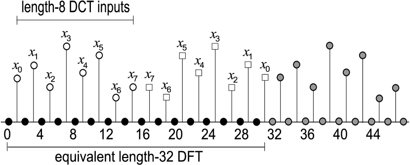
Figure 1: A DCT-II of size $N=8$ (open dots, $x_{0},\ldots,x_{7}$) is equivalent to a size-$4N$ DFT via interleaving with zeros (black dots) and extending in an even (squares) periodic (gray) sequence.

This is illustrated by an example, for $N=8$, in figure 1. The eight inputs of the DCT are shown as open dots, which are interleaved with zeros (black dots) and extended to an even (squares) periodic (gray dots) sequence of length $4N=32$ corresponding to the DFT. (The type-II DCT is distinguished from the other DCT types by the fact that it is even about both the left and right boundaries of the original data, and the symmetry points fall halfway in between pairs of the original data points.) We will refer, below, to this figure in order to illustrate what happens when an FFT algorithm is applied to this real-symmetric zero-interleaved data.

III Conjugate-pair FFT and DCT-II

Although the previous minimum flop count for DCT-II algorithms can be derived from the ordinary split-radix FFT algorithm [6, 7] (and it can also be derived in other ways [18, 19, 20, 21, 12, 22, 13, 23, 24, 25, 26]), here we will do the same thing using a variant dubbed the “conjugate-pair” split-radix FFT. This algorithm was originally proposed to reduce the number of flops [2], but was later shown to have the same flop count as ordinary split-radix [3, 4, 5]. It turns out, however, that the conjugate-pair algorithm exposes symmetries in the multiplicative factors that can be exploited to reduce the flop count by an appropriate rescaling [1], which we will employ in the following sections.

III-A Conjugate-pair split-radix FFT

Starting with the DFT of equation (3), the decimation-in-time conjugate-pair FFT splits it into three smaller DFTs: one of size $N/2$ of the even-indexed inputs, and two of size $N/4$:

$$X_{k}=\sum_{n_{2}=0}^{N/2-1}\omega_{N/2}^{n_{2}k}x_{2n_{2}}+\omega_{N}^{k}\sum_{n_{4}=0}^{N/4-1}\omega_{N/4}^{n_{4}k}x_{4n_{4}+1}\\ +\omega_{N}^{-k}\sum_{n_{4}=0}^{N/4-1}\omega_{N/4}^{n_{4}k}x_{4n_{4}-1},$$ (8)

where the indices $4n_{4}\pm 1$ are computed modulo $N$. [In contrast, the ordinary split-radix FFT uses $x_{4n_{4}+3}$ for the third sum (a cyclic shift of $x_{4n_{4}-1}$), with a corresponding multiplicative “twiddle” factor of $\omega_{N}^{3k}$.] This decomposition is repeated recursively (until base cases of size $N=1$ or $N=2$, not shown, are reached), as shown by the pseudo-code in Algorithm 1.

0:   $X_{k=0..N-1}\leftarrow\operatorname{\mathbf{splitfft}}_{N}\left(x_{n}\right)$:

  $U_{k_{2}=0\ldots N/2-1}\leftarrow\operatorname{\mathbf{splitfft}}_{N/2}\left(x_{2n_{2}}\right)$

  $Z_{k_{4}=0\ldots N/4-1}\leftarrow\operatorname{\mathbf{splitfft}}_{N/4}\left(x_{4n_{4}+1}\right)$

  $Z^{\prime}_{k_{4}=0\ldots N/4-1}\leftarrow\operatorname{\mathbf{splitfft}}_{N/4}\left(x_{4n_{4}-1}\right)$

  for $k=0$ to $N/4-1$ do

     $X_{k}\leftarrow U_{k}+\left(\omega_{N}^{k}Z_{k}+\omega_{N}^{-k}Z^{\prime}_{k}\right)$

     $X_{k+N/2}\leftarrow U_{k}-\left(\omega_{N}^{k}Z_{k}+\omega_{N}^{-k}Z^{\prime}_{k}\right)$

     $X_{k+N/4}\leftarrow U_{k+N/4}-i\left(\omega_{N}^{k}Z_{k}-\omega_{N}^{-k}Z^{\prime}_{k}\right)$

     $X_{k+3N/4}\leftarrow U_{k+N/4}+i\left(\omega_{N}^{k}Z_{k}-\omega_{N}^{-k}Z^{\prime}_{k}\right)$

  end for

Algorithm 1 Standard conjugate-pair split-radix FFT algorithm of size $N$. Special-case optimizations for $k=0$ and $k=N/8$, as well as the base cases, are omitted for simplicity.

Here, we denote the results of the three sub-transforms of size $N/2$, $N/4$, and $N/4$ by $U_{k}$, $Z_{k}$, and $Z_{k}^{\prime}$, respectively. The number of flops required by this algorithm, after certain simplifications (common subexpression elimination and constant folding, and special-case simplifications of the constants for $k=0$ and $k=N/8$) and not counting data-independent operations like the computation of $\omega_{N}^{k}$, is $4N\log_{2}N-6N+8$, identical to ordinary split radix.

In the following sections, we will have to exploit further simplifications for the case where the inputs $x_{n}$ are real. In this case, $X_{k}=X_{-k}^{*}$ (where $\ast$ denotes complex conjugation) and one can save slightly more than half of the flops, both in the ordinary split-radix [7, 48] and in the conjugate-pair split-radix [1], by eliminating redundant operations, to achieve a flop count of $2N\log_{2}N-4N+6$. Specifically, one need only compute the outputs for $0\leq k\leq N/2$ (where the $k=0$ and $k=N/2$ outputs are purely real), and the corresponding algorithm is shown in Algorithm 2.

0:   $X_{k=0..N/2}\leftarrow\operatorname{\mathbf{rsplitfft}}_{N}\left(x_{n}\right)$:

  $U_{k_{2}=0\ldots N/4}\leftarrow\operatorname{\mathbf{rsplitfft}}_{N/2}\left(x_{2n_{2}}\right)$

  $Z_{k_{4}=0\ldots N/8}\leftarrow\operatorname{\mathbf{rsplitfft}}_{N/4}\left(x_{4n_{4}+1}\right)$

  $Z^{\prime}_{k_{4}=0\ldots N/8}\leftarrow\operatorname{\mathbf{rsplitfft}}_{N/4}\left(x_{4n_{4}-1}\right)$

  for $k=0$ to $N/8$ do

     $X_{k}\leftarrow U_{k}+\left(\omega_{N}^{k}Z_{k}+\omega_{N}^{-k}Z^{\prime}_{k}\right)$

     $X_{k+N/4}\leftarrow U_{N/4-k}^{\ast}-i\left(\omega_{N}^{k}Z_{k}-\omega_{N}^{-k}Z^{\prime}_{k}\right)$

     $X_{N/4-k}\leftarrow U_{N/4-k}-i\left(\omega_{N}^{k}Z_{k}-\omega_{N}^{-k}Z_{k}^{\prime}\right)^{\ast}$

     $X_{N/2-k}\leftarrow U_{k}^{\ast}-\left(\omega_{N}^{k}Z_{k}+\omega_{N}^{-k}Z_{k}^{\prime}\right)^{\ast}$

  end for

Algorithm 2 Standard conjugate-pair split-radix FFT algorithm of size $N$ as in Algorithm 1, but specialized for the case of real inputs. Special-case optimizations for $k=0$ and $k=N/8$, as well as the base cases, are omitted for simplicity.

Again, for simplicity we do not show special-case optimizations for $k=0$ and $k=N/8$, so it may appear that the $X_{N/8}$, $X_{N/4}$, and $X_{3N/8}$ outputs are computed twice. To derive Algorithm 2, one exploits two facts. First, the sub-transforms operate on real data and therefore have conjugate-symmetric output. Second, the twiddle factors in Algorithm 1 have some redundancy because of the identity $\omega_{N}^{\pm(N/4-k)}=\mp i\omega_{N}^{\mp k}$, which allows us to share twiddle factors between $k$ and $N/4-k$ in the original loop.

III-B Fast DCT-II via split-radix FFT

Before we derive our fast DCT-II with a reduced flop count, we first derive a DCT-II algorithm with the same flop count as previously published algorithms, but starting with the conjugate-pair split-radix algorithm. This algorithm will then be modified in section IV-B, below, to reduce the number of multiplications.

In eq. (5), we showed that a DCT-II of size $N$, with inputs $x_{n}$ and outputs $C_{k}$, can be expressed as the first $N$ outputs of a DFT of size $\tilde{N}=4N$ of real-even inputs $\tilde{x}_{n}$. [Therefore, $N$ in eq. (8) above and in the surrounding text are replaced below by $\tilde{N}$.] Now, consider what happens when we evaluate this DFT via the conjugate-pair split decomposition in eq. (8) and Algorithm 2. In this algorithm, we compute three smaller DFTs. First, $U_{k}$ is the DFT of size $\tilde{N}/2=2N$ of the $\tilde{x}_{2n}$ inputs, but these are all zero and so $U_{k}$ is zero. Second, $Z{}_{k}$ is the DFT of size $\tilde{N}/4=N$ of the $\tilde{x}_{4n+1}$ inputs (where $4n+1$ is evaluated modulo $\tilde{N}$), which by eq. (7) correspond to the original data $x_{n}$ by the formula:

$$\tilde{y}_{n}=\tilde{x}_{4n+1}=\left\{\begin{array}[]{cc}x_{2n}&0\leq n<N/2\\ x_{2N-1-2n}&N/2\leq n<N\end{array}\right.,$$ (9)

where we have denoted them by $\tilde{y}_{n}$ ($0\leq n<N$) for convenience. That is, $Z{}_{k}$ is the real-input DFT of the even-indexed elements of $x_{n}$ followed by the odd-indexed elements of $x_{n}$ in reverse order. For example, this is shown for $N=8$ in figure 2 with the circled points corresponding to the $\tilde{y}_{n}$, which are clearly the even-indexed $x_{n}$ followed by the odd-indexed $x_{n}$ in reverse.

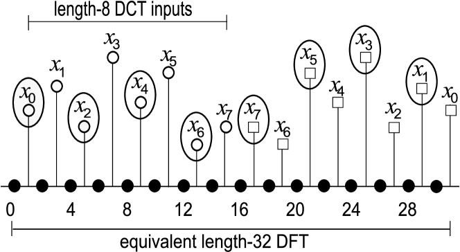
Figure 2: The DCT-II of $N=8$ points $x_{n}$ (open dots) is computed, in a conjugate-pair FFT of the $\tilde{N}=32$ extended data $\tilde{x}_{n}$ (squares) from figure 1, via the DFT $Z_{k}$ of the circled points $\tilde{x}_{4n+1}$, corresponding to the even-indexed $x_{n}$ followed by the odd-indexed $x_{n}$.

The second DFT, $Z_{k}^{\prime}$, of size $\tilde{N}/4=N$ is redundant: it is the DFT of $\tilde{x}_{4n-1}$, but by the even symmetry of $\tilde{x}_{n}$ this is equal to $\tilde{x}_{4(-n)+1}$, and therefore $Z_{k}^{\prime}=Z_{k}^{*}$ (the complex conjugate of $Z_{k}$).

Therefore, a fast DCT-II is obtained merely by computing a single real-input DFT of size $N$ to obtain $Z_{k}=Z_{N-k}^{*}$, and then combining this according to Algorithm 2 to obtain $C_{k}=X_{k}$ for $k=0\ldots N-1$. In particular, in the loop of Algorithm 2, all but the $X_{k}$ and $X_{\tilde{N}/4-k}$ terms correspond to subscripts $\geq N$ and are not needed. Moreover, we obtain

$$X_{k} =\omega_{\tilde{N}}^{k}Z_{k}+\omega_{\tilde{N}}^{-k}Z_{k}^{*}=2\Re\left(\omega_{4N}^{k}Z_{k}\right),$$

$$X_{N-k} =-i\left(\omega_{\tilde{N}}^{k}Z_{k}-\omega_{\tilde{N}}^{-k}Z_{k}^{*}\right)^{*}=-2\Im\left(\omega_{4N}^{k}Z_{k}\right).$$

The resulting algorithm, including the special-case optimizations for $k=0$ (where $\omega_{4N}^{0}=1$ and $Z_{0}$ is real) and $k=N/2$ (where $\omega_{4N}^{N/2}=(1-i)/\sqrt{2}$ and $Z_{N/2}$ is real), is shown in Algorithm 3.

0:   $C_{k=0..N-1}\leftarrow\operatorname{\mathbf{splitdctII}}_{N}\left(x_{n}\right)$:

  for $n=0$ to $N/2-1$ do

     $\tilde{y}_{n}\leftarrow x_{2n}$

     $\tilde{y}_{N-1-n}\leftarrow x_{2n+1}$

  end for

  $Z_{k=0\ldots N/2}\leftarrow\operatorname{\mathbf{rsplitfft}}_{N}\left(\tilde{y}_{n}\right)$

  $C_{0}\leftarrow 2Z_{0}$

  for $k=1$ to $N/2-1$ do

     $C_{k}\leftarrow 2\Re\left(\omega_{4N}^{k}Z_{k}\right)$

     $C_{N-k}\leftarrow-2\Im\left(\omega_{4N}^{k}Z_{k}\right)$

  end for

  $C_{N/2}\leftarrow\sqrt{2}Z_{N/2}$

Algorithm 3 Fast DCT-II algorithm, matching previous best flop count, derived from Algorithm 2 by discarding redundant operations.

In fact, Algorithm 3 is equivalent to an algorithm derived in a different way by various authors [30, 33] to express a DCT-II in terms of a real-input DFT of the same length. Here, we see that this algorithm is exactly equivalent to a conjugate-pair split-radix FFT of length $4N$. Previous authors obtained a suboptimal flop count $\frac{5}{2}N\log_{2}N+O(N)$ for the DCT-II using this algorithm [33] only because they used a suboptimal real-input DFT for the subtransform (split-radix being then almost unknown). Using a real-input split-radix DFT to compute $Z_{k}$, the flop count for $Z_{k}$ is $2N\log_{2}N-4N+6$ from above. To get the total flop count for Algorithm 3, we need to add $N/2-1$ general complex multiplications by $2\omega_{4N}^{k}$ (6 flops each) plus two real multiplications (2 flops), for a total of $2N\log_{2}N-N+2$ flops. This matches the best-known flop count in the literature (where the $+2$ can be removed merely by choosing a different normalization as discussed in section V).

IV New FFT and DCT-II

In this section, we first review the new FFT algorithm introduced in our previous work based on a recursive rescaling of the conjugate-pair FFT [1], and then apply it to derive a fast DCT-II algorithm as in the previous section.

IV-A New FFT

Based on the conjugate-pair split-radix FFT from section III, a new FFT algorithm with a reduced number of flops can be derived by scaling the subtransforms [1]. We will not reproduce the derivation here, but will simply summarize the results. In particular, the original conjugate-pair split-radix Algorithm 1 is split into four mutually recursive subroutines, each of which has the same split-radix structure but computes a DFT scaled by a different factor. These algorithms are shown in Algorithm 4 for the case of complex inputs, and in Algorithm 5 specialized for real inputs, in both of which the scaling factors are combined with the twiddle factors $\omega_{N}^{k}$ to reduce the total number of multiplications compared to Algorithms 1 and 2, respectively.

0:   $X_{k=0..N-1}\leftarrow\operatorname{\mathbf{newfftS}}_{N}^{\ell}\left(x_{n}\right)$: {computes DFT / $s_{\ell N,k}$ for $\ell=0,1,2$}

  $U_{k_{2}=0\ldots N/2-1}\leftarrow\operatorname{\mathbf{newfftS}}_{N/2}^{2\ell}\left(x_{2n_{2}}\right)$

  $Z_{k_{4}=0\ldots N/4-1}\leftarrow\operatorname{\mathbf{newfftS}}_{N/4}^{1}\left(x_{4n_{4}+1}\right)$

  $Z^{\prime}_{k_{4}=0\ldots N/4-1}\leftarrow\operatorname{\mathbf{newfftS}}_{N/4}^{1}\left(x_{4n_{4}-1}\right)$

  for $k=0$ to $N/4-1$ do

     $X_{k}\leftarrow U_{k}+\left(t_{N,k}Z_{k}+t_{N,k}^{*}Z^{\prime}_{k}\right)\cdot(s_{N,k}/s_{\ell N,k})$

     $X_{k+N/2}\leftarrow U_{k}-\left(t_{N,k}Z_{k}+t_{N,k}^{*}Z^{\prime}_{k}\right)\cdot(s_{N,k}/s_{\ell N,k})$

     $X_{k+N/4}\leftarrow U_{k+N/4}$     $-\>i\left(t_{N,k}Z_{k}-t_{N,k}^{*}Z^{\prime}_{k}\right)\cdot(s_{N,k}/s_{\ell N,k+N/4})$

     $X_{k+3N/4}\leftarrow U_{k+N/4}$     $+\>i\left(t_{N,k}Z_{k}-t_{N,k}^{*}Z^{\prime}_{k}\right)\cdot(s_{N,k}/s_{\ell N,k+N/4})$

  end for

   $X_{k=0..N-1}\leftarrow\operatorname{\mathbf{newfftS4}}_{N}\left(x_{n}\right)$: {computes DFT / $s_{4N,k}$}

  $U_{k_{2}=0\ldots N/2-1}\leftarrow\operatorname{\mathbf{newfftS}}_{N/2}^{2}\left(x_{2n_{2}}\right)$

  $Z_{k_{4}=0\ldots N/4-1}\leftarrow\operatorname{\mathbf{newfftS}}_{N/4}^{1}\left(x_{4n_{4}+1}\right)$

  $Z^{\prime}_{k_{4}=0\ldots N/4-1}\leftarrow\operatorname{\mathbf{newfftS}}_{N/4}^{1}\left(x_{4n_{4}-1}\right)$

  for $k=0$ to $N/4-1$ do

     $X_{k}\leftarrow\left[U_{k}+\left(t_{N,k}Z_{k}+t_{N,k}^{*}Z^{\prime}_{k}\right)\right]\cdot(s_{N,k}/s_{4N,k})$

     $X_{k+N/2}\leftarrow\left[U_{k}-\left(t_{N,k}Z_{k}+t_{N,k}^{*}Z^{\prime}_{k}\right)\right]$                 $\cdot\>(s_{N,k}/s_{4N,k+N/2})$

     $X_{k+N/4}\leftarrow\left[U_{k+N/4}-i\left(t_{N,k}Z_{k}-t_{N,k}^{*}Z^{\prime}_{k}\right)\right]$                 $\cdot\>(s_{N,k}/s_{4N,k+N/4})$

     $X_{k+3N/4}\leftarrow\left[U_{k+N/4}+i\left(t_{N,k}Z_{k}-t_{N,k}^{*}Z^{\prime}_{k}\right)\right]$                 $\cdot\>(s_{N,k}/s_{4N,k+3N/4})$

  end for

Algorithm 4 New FFT algorithm [1] of length $N$ (divisible by $4$). The sub-transforms $\operatorname{\mathbf{newfftS}}_{N}^{\ell}\left(x\right)$ for $\ell\neq 0$ are scaled by $s_{\ell N,k}$, respectively, while $\ell=0$ is the final unscaled DFT ($s_{0,k}=1$). Special-case optimizations for $k=0$ and $k=N/8$ are not shown.

0:   $X_{k=0..N/2}\leftarrow\operatorname{\mathbf{rnewfftS}}_{N}^{\ell}\left(x_{n}\right)$: {computes DFT / $s_{\ell N,k}$ for $\ell=0,1,2$}

  $U_{k_{2}=0\ldots N/4}\leftarrow\operatorname{\mathbf{rnewfftS}}_{N/2}^{2\ell}\left(x_{2n_{2}}\right)$

  $Z_{k_{4}=0\ldots N/8}\leftarrow\operatorname{\mathbf{rnewfftS}}_{N/4}^{1}\left(x_{4n_{4}+1}\right)$

  $Z^{\prime}_{k_{4}=0\ldots N/8}\leftarrow\operatorname{\mathbf{rnewfftS}}_{N/4}^{1}\left(x_{4n_{4}-1}\right)$

  for $k=0$ to $N/8$ do

     $X_{k}\leftarrow U_{k}+\left(t_{N,k}Z_{k}+t_{N,k}^{*}Z^{\prime}_{k}\right)\cdot(s_{N,k}/s_{\ell N,k})$

     $X_{k+N/4}\leftarrow U_{N/4-k}^{\ast}$     $-\>i\left(t_{N,k}Z_{k}-t_{N,k}^{*}Z^{\prime}_{k}\right)\cdot(s_{N,k}/s_{\ell N,k+N/4})$

     $X_{N/4-k}\leftarrow U_{N/4-k}$     $-\>i\left(t_{N,k}Z_{k}-t_{N,k}^{*}Z_{k}^{\prime}\right)^{*}\cdot(s_{N,k}/s_{\ell N,k+N/4})$

     $X_{N/2-k}\leftarrow U_{k}^{*}$     $-\left(t_{N,k}Z_{k}+t_{N,k}^{*}Z_{k}^{\prime}\right)^{*}\cdot(s_{N,k}/s_{\ell N,k})$

  end for

   $X_{k=0..N/2}\leftarrow\operatorname{\mathbf{rnewfftS4}}_{N}\left(x_{n}\right)$: {computes DFT / $s_{4N,k}$}

  $U_{k_{2}=0\ldots N/4}\leftarrow\operatorname{\mathbf{rnewfftS}}_{N/2}^{2}\left(x_{2n_{2}}\right)$

  $Z_{k_{4}=0\ldots N/8}\leftarrow\operatorname{\mathbf{rnewfftS}}_{N/4}^{1}\left(x_{4n_{4}+1}\right)$

  $Z^{\prime}_{k_{4}=0\ldots N/8}\leftarrow\operatorname{\mathbf{rnewfftS}}_{N/4}^{1}\left(x_{4n_{4}-1}\right)$

  for $k=0$ to $N/8$ do

     $X_{k}\leftarrow\left[U_{k}+\left(t_{N,k}Z_{k}+t_{N,k}^{*}Z^{\prime}_{k}\right)\right]\cdot(s_{N,k}/s_{4N,k})$

     $X_{k+N/4}\leftarrow\left[U_{N/4-k}^{*}-i\left(t_{N,k}Z_{k}-t_{N,k}^{*}Z^{\prime}_{k}\right)\right]$                 $\cdot\>(s_{N,k}/s_{4N,k+N/4})$

     $X_{N/4-k}\leftarrow\left[U_{N/4-k}-i\left(t_{N,k}Z_{k}-t_{N,k}^{*}Z_{k}^{\prime}\right)^{*}\right]$                 $\cdot\>(s_{N,k}/s_{4N,N/4-k})$

     $X_{N/2-k}\leftarrow\left[U_{k}^{*}-\left(t_{N,k}Z_{k}+t_{N,k}^{*}Z_{k}^{\prime}\right)^{*}\right]$                 $\cdot\>(s_{N,k}/s_{4N,N/2-k})$

  end for

Algorithm 5 New FFT algorithm of size $N$ (divisible by $4$), as in Algorithm 4 but specialized for the case of real inputs. The sub-transforms $\operatorname{\mathbf{rnewfftS}}_{N}^{\ell}\left(x\right)$ for $\ell\neq 0$ are scaled by $s_{\ell N,k}$, respectively, while $\ell=0$ is the final unscaled DFT ($s_{0,k}=1$). Special-case optimizations for $k=0$ and $k=N/8$ are not shown.

Again, special cases for $k=0$ and $k=N/8$, as well as the $N=1,2$ base cases and obvious simplifications such as common-subexpression elimination, are not shown for simplicity.

The key aspect of these algorithms is the scale factor $s_{N,k}$, where the subtransforms compute the DFT scaled by $1/s_{\ell N,k}$ for $\ell=1,2,4$. (The $\ell=0,1,2$ subroutines are condensed into one in Algorithms 4–5, by making $\ell$ a variable, but in practice they need to be implemented separately in order to exploit the special cases of the scale factor [1]. The $\ell=4$ case is written separately because it is factorized differently.) This scale factor is defined for $N=2^{m}$ by the following recurrence, where $k_{4}=k$ mod $\frac{N}{4}$:

$$s_{N=2^{m},k}=\left\{\begin{array}[]{cl}1&\quad\textrm{for }N\leq 4\\ s_{N/4,k_{4}}\cos(2\pi k_{4}/N)&\quad\textrm{for }k_{4}\leq N/8\\ s_{N/4,k_{4}}\sin(2\pi k_{4}/N)&\quad\textrm{otherwise}\end{array}\right..$$ (10)

This definition has the properties: $s_{N,0}=1$, $s_{N,k+N/4}=s_{N,k}$, and $s_{N,N/4-k}=s_{N,k}$. Also, $s_{N,k}>0$ and decays rather slowly with $N$: $s_{N,k}$ has an $\Omega(N^{\log_{4}\cos(\pi/5)})$ asymptotic lower bound [1]. When these scale factors are combined with the twiddle factors $\omega_{N}^{k}$, we obtain terms of the form

$$t_{N,k}=\omega_{N}^{k}\frac{s_{N/4,k}}{s_{N,k}},$$ (11)

which is always a complex number of the form $\pm 1\pm i\tan\frac{2\pi k}{N}$ or $\pm\cot\frac{2\pi k}{N}\pm i$ and can therefore be multiplied with two fewer real multiplications than are required to multiply by $\omega_{N}^{k}$. Because of the symmetry $s_{N,N/4-k}=s_{N,k}$, it is possible to specialize Algorithm 4 for real data in the same way as in Algorithm 2, because the scale factor preserves the conjugate symmetry $X_{k}=X_{N-k}^{*}$ of the outputs of all subtransforms [1].

The resulting flop count, for arbitrary complex data $x_{n}$, is then reduced from $4N\log_{2}N-6N+8$ to

$$\frac{34}{9}N\log_{2}N-\frac{124}{27}N-2\log_{2}N\\ -\frac{2}{9}(-1)^{\log_{2}N}\log_{2}N+\frac{16}{27}(-1)^{\log_{2}N}+8.$$ (12)

In particular, assuming that complex multiplications are implemented as four real multiplications and two real additions, then the savings are purely in the number of real multiplications. The number $M(N)$ of real multiplications saved over ordinary split radix is given by:

$$M(N)=\frac{2}{9}N\log_{2}N-\frac{38}{27}N+2\log_{2}N\\ +\frac{2}{9}(-1)^{\log_{2}N}\log_{2}N-\frac{16}{27}(-1)^{\log_{2}N}.$$ (13)

If the data are purely real, it was shown that $M(N)/2$ multiplications are saved over the corresponding real-input split-radix algorithm [1]. These flop counts are to compute the original, unscaled definition of the DFT. If one is allowed to scale the outputs by any factor desired, then scaling by $1/s_{N,k}$ [corresponding to $\operatorname{\mathbf{newfftS}}_{N}^{1}\left(x_{n}\right)$ in Algorithm 4], saves an additional $M_{S}(N)-M(N)\geq 0$ multiplications for complex inputs, where:

$$M_{S}(N)=\frac{2}{9}N\log_{2}N-\frac{20}{27}N\\ +\frac{2}{9}(-1)^{\log_{2}N}\log_{2}N-\frac{7}{27}(-1)^{\log_{2}N}+1.$$ (14)

For real inputs, one similarly saves $M_{S}(N)/2$ flops for $\operatorname{\mathbf{rnewfftS}}_{N}^{1}\left(x_{n}\right)$ operating on real $x_{n}$ in Algorithm 5.

Although the division by a cosine or sine in the scale factor may, at first glance, seem as if it may exacerbate floating-point errors, this is not the case. Cooley–Tukey based FFT algorithms have $O(\sqrt{\log N})$ root-mean-square error growth, and $O(\log N)$ error bounds, in finite-precision floating-point arithmetic (assuming that the trigonometric constants are precomputed accurately) [49, 50, 51], and the new FFT is no different [1]. The reason for this is straightforward: it never adds or subtracts scaled and unscaled values. Instead, wherever the original FFT would compute $a+b$, the new FFT computes $s\cdot(a+b)$ for some fixed scale factor $s$.

IV-B Fast DCT-II from new FFT

To derive the new DCT-II algorithm based on the new FFT of the previous section, we follow exactly the same process as in Sec. III-B. We express the DCT-II of length $N$ in terms of a DFT of length $4N$, apply the FFT algorithm 5, and discard the redundant operations. As before, the $U_{k}$ subtransform is identically zero, $Z_{k}$ is the transform of the even-indexed elements of $x_{n}$ followed by the odd-indexed elements in reverse order, and $Z_{k}^{\prime}=Z_{N-k}^{*}$ is redundant.

0:   $C_{k=0..N-1}\leftarrow\operatorname{\mathbf{newdctII}}_{N}\left(x_{n}\right)$:

  for $n=0$ to $N/2-1$ do

     $\tilde{y}_{n}\leftarrow x_{2n}$

     $\tilde{y}_{N-1-n}\leftarrow x_{2n+1}$

  end for

  $Z_{k=0..N/2}\leftarrow\operatorname{\mathbf{rnewfftS}}_{N}^{1}\left(\tilde{y}_{n}\right)$

  $C_{0}\leftarrow 2Z_{0}$

  for $k=1$ to $N/2-1$ do

     $C_{k}\leftarrow 2\Re\left(\omega_{4N}^{k}s_{N,k}Z_{k}\right)$

     $C_{N-k}\leftarrow-2\Im\left(\omega_{4N}^{k}s_{N,k}Z_{k}\right)$

  end for

  $C_{N/2}\leftarrow\sqrt{2}Z_{N/2}$

Algorithm 6 New DCT-II algorithm of size $N=2^{m}$, based on discarding redundant operations from the new FFT algorithm of size $4N$, achieving new record flop count.

The resulting algorithm is shown in Algorithm 6, and differs from the original fast DCT-II of Algorithm 3 in only two ways. First, instead of calling the ordinary split-radix (or conjugate-pair) FFT for the subtransform, it calls $\operatorname{\mathbf{newfftS}}_{N}\left(x_{n}\right)$. Second, because this subtransform is scaled by $1/s_{N,k}$, the twiddle factor $\omega_{4N}^{k}$ in Algorithm 6 is multiplied by $s_{N,k}$.

To derive the flop count for Algorithm 6, we merely need to add the flop count for the subtransform [which saves $M_{S}(N)/2=\frac{1}{9}N\log_{2}N+O(N)$ flops, from eq. (14), compared to ordinary real-input split radix] with the number of flops in the loop, where the latter is exactly the same as for Algorithm 3 because the products $\omega_{4N}^{k}s_{N,k}$ can be precomputed. Therefore, we save a total of $M_{S}(N)/2$ flops compared to the previous best flop count of $2N\log_{2}N-N+2$, resulting in the flop count of eq. (1). This formula matches the flop count that was achieved by an automatic code generator in Ref. [1].

Because the new DCT algorithm is mathematically merely a special set of inputs for the underlying FFT, it will have the same favorable logarithmic error bounds as discussed in the previous section.

V Normalizations

In the above definition of DCT-II, we use a scale factor “2” in front of the summation in order to make the DCT-II directly equivalent to the corresponding DFT. But in some circumstances, it is useful to multiply by other factors, and different normalizations lead to slightly different flop counts. For example, one could use the unitary normalization from eq. (2), which replaces $2$ by $\sqrt{2/N}$ or $\sqrt{1/N}$ (for $k=0$) and requires the same number of flops. If one uses the unitary normalization multiplied by $\sqrt{N}$, then one saves two multiplications in the $k=0$ and $k=N/2$ terms (in this normalization, $C_{0}=Z_{0}$ and $C_{N/2}=Z_{N/2}$) for both Algorithm 3 and Algorithm 6. (This leads to a commonly quoted $2N\log_{2}N-N$ formula for the previous flop count.)

It is also common to compute a DCT-II with scaled outputs, e.g. for the JPEG image-compression standard where an arbitrary scaling can be absorbed into a subsequent quantization step [43], and in this case the scaling can save 8 multiplications [42] over the 42 flops required for an unitary 8-point DCT-II. Since our $\operatorname{\mathbf{newfftS}}_{N}^{1}\left(x_{n}\right)$ attempts to be the optimally scaled FFT, we should be able to derive this scaled DCT-II by using $\operatorname{\mathbf{rnewfftS}}_{N}^{1}\left(x_{n}\right)/2$ for our length-$4N$ DFT instead of $\operatorname{\mathbf{rnewfftS}}_{N}^{0}\left(x\right)$, and again pruning the redundant operations. Doing so, we obtain an algorithm identical to Algorithm 6 except that $2\omega_{4N}^{k}s_{N,k}$ is replaced by $t_{4N,k}$, which requires fewer multiplications, and also we now obtain $C_{0}=Z_{0}$ and $C_{N/2}=Z_{N/2}$. This algorithm computes $C_{k}/2s_{4N,k}$ instead of $C_{k}$. In particular, we save exactly $N$ multiplications over Algorithm 6, which matches the result by Ref. [42] for $N=8$ but generalizes it to all $N$. This savings of $N$ multiplications for a scaled DCT-II also matches the flop count that was achieved by an automatic code generator in Ref. [1].

VI Fast DCT-III, DST-II, and DST-III

Given any algorithm for the DCT-II, one can immediately obtain algorithms for the DCT-III, DST-II, and DST-III with exactly the same number of arithmetic operations. In this way, any improvement in the DCT-II, such as the one described in this paper, immediately leads to improved algorithms for those transforms and vice versa. In this section, we review the equivalence between those transforms.

VI-A DCT-III

To obtain a DCT-III algorithm from a DCT-II algorithm, one can exploit two facts. First, the DCT-III, viewed as a matrix, is simply the transpose of the DCT-II matrix. Second, any linear algorithm can be viewed as a linear network, and the transpose operation is computed by the network transposition of this algorithm [52]. To review, a linear network represents the algorithm by a directed acyclic graph, where the edges represent multiplications by constants and the vertices represent additions of the incoming edges. Network transposition simply consists of reversing the direction of every edge. We prove below that the transposed network requires the same number of additions and multiplications for networks with the same number of inputs and outputs, and therefore the DCT-III can be computed in the same number of flops as the DCT-II by the transposed algorithm. The DCT-III corresponding to the transpose of eq. (4) is

$$C{}_{k}^{\mathrm{T}}=2\sum_{n=0}^{N-1}x_{n}\cos\left[\frac{\pi}{N}n\left(k+\frac{1}{2}\right)\right].$$ (15)

Since the DCT-III is the transpose of the DCT-II, a fast DCT-III algorithm is obtained by network transposition of a fast DCT-II algorithm. For example, network transposition of a size-2 DCT-III is shown in figure. 3.

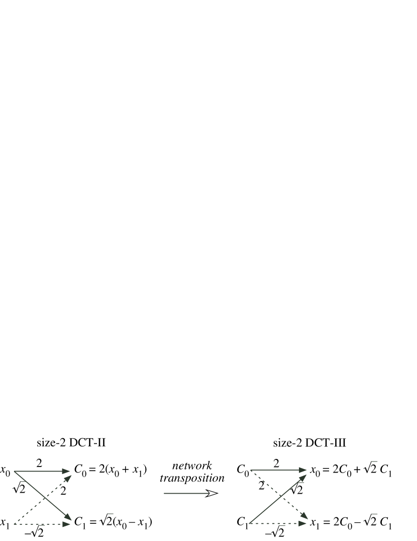
Figure 3: Example of network transposition for a size-2 DCT-II (left). When the linear network is transposed (all edges are reversed), the resulting network computes the transposed-matrix operation: a size-2 DCT-III (right).

A proof that the transposed network requires the same number of flops is as follows. Clearly, the number of multiplications, the number of edges with weight $\neq\pm 1$, is unchanged by transposition. The number of additions is given by the sum of $\operatorname{\mathrm{indegree}}-1$ for all the vertices, except for the $N$ input vertices which have indegree zero. That is, for a set $V$ of vertices and a set $E$ of edges:

# adds $$=N+\sum_{v\in V}[\operatorname{\mathrm{indegree}}(v)-1]$$

$$=N+|E|-|V|,$$ (16)

using the fact that the sum of the $\operatorname{\mathrm{indegree}}$ over all vertices is simply the number $|E|$ of edges. Because the above expression is obviously invariant under network transposition as long as $N$ is unchanged (i.e. same number of inputs and outputs), the number of additions is invariant.

More explicitly, a fast DCT-III algorithm derived from the transpose of our new Algorithm 6 is outlined in Algorithm 7. Whereas for the DCT-II we computed the real-input DFT (with conjugate-symmetric output) of the rearranged inputs $\tilde{y}_{n}$ and then post-processed the complex outputs $Z_{k}=Z_{N-k}^{*}$, now we do the reverse. We first preprocess the inputs to form a complex array $Z_{k}=Z_{N-k}^{*}$, then perform a real-output, scaled-input DFT to obtain $\tilde{y}_{k}$, and finally assign the even and odd elements of the result $C_{k}^{\mathrm{T}}$ from the first and second halves of $\tilde{y}_{k}$. Without the scale factors, this is equivalent to a well-known algorithm to express a DCT-III in terms of a realoutput DFT of the same size [30, 33]. In order to minimize the flop count once the scale factors are included, however, it is important that this real-output DFT operate on scaled inputs rather than scaled outputs, so it is intrinsically different (transposed) from Algorithm 4. The real-output (scaled, conjugate-symmetric input) version of $\operatorname{\mathbf{rnewfftS}}_{N}^{1}\left(x_{n}\right)$ can be derived by network transposition of the real-input case (since network transposition interchanges inputs and outputs). Equivalently, whereas the $\operatorname{\mathbf{rnewfftS}}_{N}^{1}\left(x_{n}\right)$ was a scaled-output decimation-in-time algorithm specialized for real inputs, the transposed algorithm $\operatorname{\mathbf{rnewfftS}}_{N}^{(\mathrm{T})\,1}\left(x_{n}\right)$ is a scaled-input decimation-in-frequency algorithm specialized for real outputs. We do not list $\operatorname{\mathbf{rnewfftS}}_{N}^{(\mathrm{T})\,1}\left(x_{n}\right)$ explicitly here, however; our main point is simply to establish that an algorithm for the DCT-III with exactly the same flop count (1) follows immediately from the new DCT-II.

0:   $D_{k=0..N-1}\leftarrow\operatorname{\mathbf{newdctIII}}_{N}\left(x_{n}\right)$:

  $Z_{0}\leftarrow 2x_{0}$

  for $n=1$ to $N/2-1$ do

     $Z_{n}\leftarrow 2\omega_{4N}^{-n}s_{N,n}(x_{n}-ix_{N-n})$

     $Z_{N-n}\leftarrow Z_{n}^{*}$

  end for

  $Z_{N/2}\leftarrow\sqrt{2}x_{N/2}$

  $\tilde{y}_{k}\leftarrow\operatorname{\mathbf{rnewfftS}}_{N}^{(\mathrm{T})\,1}\left(Z_{n}\right)$

  for $k=0$ to $N/2-1$ do

     $C_{2k}^{\mathrm{T}}\leftarrow\tilde{y}_{k}$

     $C_{2k+1}^{\mathrm{T}}\leftarrow\tilde{y}_{N-1-k}$

  end for

Algorithm 7 New DCT-III algorithm of size $N=2^{m}$, based on network transposition of Algorithm 6, with the same flop count.

There are also other ways to derive a DCT-III algorithm with the same flop count without using network transposition, of course. For example, one can again consider the DCT-III to be a real-input DFT of size $4N$ with certain symmetries (different from the DCT-II’s symmetries), and prune redundant operations from Algorithm 5, resulting in a decimation-in-time algorithm. Such a derivation is useful because it allows one to derive a scaled-output DCT-III as well, which turns out to be a subroutine of a new DCT-IV algorithm that we describe in another manuscript, currently in press [53]. However, this derivation is more complicated than the one above, resulting in four mutually recursive DCT-III subroutines, and does not lower the flop count, so we omit it here.

VI-B DST-II and DST-III

The DST-II is defined, using a unitary normalization, as:

$$S_{k}^{\mathrm{II}}=\sqrt{\frac{2-\delta_{k,N}}{N}}\sum_{n=0}^{N-1}x_{n}\sin\left[\frac{\pi}{N}\left(n+\frac{1}{2}\right)k\right]$$ (17)

for $k=1,\ldots,N$ (not $0,\ldots,N-1$). As in section II, it is more convenient to develop algorithms for an unnormalized variation:

$$S_{k}=2\sum_{n=0}^{N-1}x_{n}\sin\left[\frac{\pi}{N}\left(n+\frac{1}{2}\right)k\right]$$ (18)

similar to our normalization of $C_{k}$ and $C_{k}^{\mathrm{T}}$ above. Although we could derive fast algorithms for $S_{k}$ directly by treating it as a DFT of length $4N$ with odd symmetry, interleaved with zeros, and discarding redundant operations similar to above, it turns out there is a simpler technique. The DST-II is exactly equivalent to a DCT-II in which the outputs are reversed and every other input is multiplied by $-1$ [11, 12, 13]:

$$S_{N-k}=2\sum_{n=0}^{N-1}(-1)^{n}x_{n}\cos\left[\frac{\pi}{N}\left(n+\frac{1}{2}\right)k\right]$$ (19)

for $k=0,\ldots,N-1$. It therefore follows that a DST-II can be computed with the same number of flops as a DCT-II of the same size, assuming that multiplications by $-1$ are free—the reason for this is that sign flips can be absorbed at no cost by converting additions into subtractions or vice versa in the subsequent algorithmic steps. Therefore, our new flop count (1) immediately applies to the DST-II.

Similarly, a DST-III is given by the transpose of the DST-II (which is the inverse, for the unitary normalization). In unnormalized form, this is

$$S_{k}^{\mathrm{T}}=2\sum_{n=1}^{N}x_{n}\sin\left[\frac{\pi}{N}n\left(k+\frac{1}{2}\right)\right]$$ (20)

for $k=0,\ldots,N-1$. This must have the same number of flops as the DST-II by the network transposition argument above. Alternatively, it can also be obtained from the DCT-III by reversing the inputs and multiplying every other output by $-1$ [12]:

$$S_{k}^{\mathrm{T}}=(-1)^{k}\sum_{n=0}^{N-1}x_{N-n}\cos\left[\frac{\pi}{N}n\left(k+\frac{1}{2}\right)\right],$$ (21)

which can be obtained from $C_{k}^{T}$ with the same number of flops.

VII Conclusion

We have shown that a improved count of real additions and multiplications (flops), eq. (1), can be obtained for the DCT/DST types II/III by pruning redundant operations from a recent improved FFT algorithm. We have also shown how to save $N$ multiplications by rescaling the outputs of a DCT-II (or the inputs of a DCT-III), generalizing a well-known technique for $N=8$ [42]. However, we do not claim that our new count is optimal—it may be that further gains can be obtained by, for example, extending the rescaling technique of [1] to greater generality. In particular, as has been pointed out by other authors [8], any improvement in the arithmetic complexity or flop counts for the DFT immediately leads to corresponding improvements in DCTs/DSTs, and vice versa. Our most important result, we believe, is the fact that there suddenly appears to be new room for improvement in problems that had seen no reductions in flop counts for many years.

The question of the minimal operation counts for basic linear transformations such as DCTs and DSTs is of longstanding theoretical interest. The practical impact of a few percent improvement in flop counts, admittedly, is less clear because computation time on modern hardware is often not dominated by arithmetic [10]. Nevertheless, minimal-arithmetic hard-coded DCTs of small sizes are often used in audio and image compression [47, 43], and the availability of any new algorithm with regular structure amenable to implementation leads to rich new opportunities for performance optimization.

Similar arithmetic improvements also occur for other types of DCT and DST [1], as well as for the modified DCT (MDCT, closely related to a DCT-IV), and the explicit description of those algorithms is the subject of another manuscript currently in press [53]. We have already shown that the new exact count for the DCT-I is $2N\log_{2}N-3N+2\log_{2}N+5-M(2N)/4=\frac{17}{9}N\log_{2}N+O(N)$, where $M(N)$ is given by eq. (13) [1]. However, no new exact count for arbitrary $N=2^{m}$ has yet been published for the DCT-IV and related transforms. Again, it immediately follows that the asymptotic cost of a DCT-IV (and hence an MDCT) is reduced to $\frac{17}{9}N\log_{2}N+O(N)$ simply by applying known algorithms to express a DCT-IV in terms of a DCT-II of size $N$ [12] (although this algorithm has large numerical errors [10]) or in terms of two DCT-II/III transforms of size $N/2$ [19]. However, again we wish to establish a new lowest-known upper bound for the exact count of operations of the DCT-IV, and not just the asymptotic constant factor. (It turns out that the DCT-IV algorithm obtained by pruning redundant computations from our new FFT, this time of symmetric data with size $8N$ [10], is closely related to the algorithm by Wang et al. [19], just as as the algorithm for the DCT-II in this paper was closely related to a known algorithm derived by other means [30, 33].)

This work was supported in part by a grant from the MIT Undergraduate Research Opportunities Program. The authors are also grateful to M. Frigo, co-author of FFTW with S. G. Johnson [10], for many helpful discussions.

References

- [1] S. G. Johnson and M. Frigo, “A modified split-radix FFT with fewer arithmetic operations,” IEEE Trans. Signal Processing, vol. 55, no. 1, pp. 111–119, 2007.
- [2] I. Kamar and Y. Elcherif, “Conjugate pair fast Fourier transform,” Electron. Lett., vol. 25, no. 5, pp. 324–325, 1989.
- [3] R. A. Gopinath, “Comment: Conjugate pair fast Fourier transform,” Electron. Lett., vol. 25, no. 16, p. 1084, 1989.
- [4] H.-S. Qian and Z.-J. Zhao, “Comment: Conjugate pair fast Fourier transform,” Electron. Lett., vol. 26, no. 8, pp. 541–542, 1990.
- [5] A. M. Krot and H. B. Minervina, “Comment: Conjugate pair fast Fourier transform,” Electron. Lett., vol. 28, no. 12, pp. 1143–1144, 1992.
- [6] M. Vetterli and H. J. Nussbaumer, “Simple FFT and DCT algorithms with reduced number of operations,” Signal Processing, vol. 6, no. 4, pp. 267–278, 1984.
- [7] P. Duhamel, “Implementation of “split-radix” FFT algorithms for complex, real, and real-symmetric data,” IEEE Trans. Acoust., Speech, Signal Processing, vol. 34, no. 2, pp. 285–295, 1986.
- [8] P. Duhamel and M. Vetterli, “Fast Fourier transforms: a tutorial review and a state of the art,” Signal Processing, vol. 19, pp. 259–299, April 1990.
- [9] R. Vuduc and J. Demmel, “Code generators for automatic tuning of numerical kernels: experiences with FFTW,” in Proc. Semantics, Application, and Implementation of Code Generators Workshop, (Montreal), Sept. 2000.
- [10] M. Frigo and S. G. Johnson, “The design and implementation of FFTW3,” Proc. IEEE, vol. 93, no. 2, pp. 216–231, 2005.
- [11] Z. Wang, “A fast algorithm for the discrete sine transform implemented by the fast cosine transform,” IEEE Trans. Acoust., Speech, Signal Processing, vol. 30, no. 5, pp. 814–815, 1982.
- [12] S. C. Chan and K. L. Ho, “Direct methods for computing discrete sinusoidal transforms,” IEE Proceedings F, vol. 137, no. 6, pp. 433–442, 1990.
- [13] P. Lee and F.-Y. Huang, “Restructured recursive DCT and DST algorithms,” IEEE Trans. Signal Processing, vol. 42, no. 7, pp. 1600–1609, 1994.
- [14] R. Yavne, “An economical method for calculating the discrete Fourier transform,” in Proc. AFIPS Fall Joint Computer Conf., vol. 33, pp. 115–125, 1968.
- [15] P. Duhamel and H. Hollmann, “Split-radix FFT algorithm,” Electron. Lett., vol. 20, no. 1, pp. 14–16, 1984.
- [16] J. B. Martens, “Recursive cyclotomic factorization—a new algorithm for calculating the discrete Fourier transform,” IEEE Trans. Acoust., Speech, Signal Processing, vol. 32, no. 4, pp. 750–761, 1984.
- [17] T. Lundy and J. Van Buskirk, “A new matrix approach to real FFTs and convolutions of length ,” Computing, vol. 80, no. 1, pp. 23–45, 2007.
- [18] B. G. Lee, “A new algorithm to compute the discrete cosine transform,” IEEE Trans. Acoust., Speech, Signal Processing, vol. 32, no. 6, pp. 1243–1245, 1984.
- [19] Z. Wang, “On computing the discrete Fourier and cosine transforms,” IEEE Trans. Acoust., Speech, Signal Processing, vol. 33, no. 4, pp. 1341–1344, 1985.
- [20] N. Suehiro and M. Hatori, “Fast algorithms for the DFT and other sinusoidal transforms,” IEEE Trans. Acoust., Speech, Signal Processing, vol. 34, no. 3, pp. 642–644, 1986.
- [21] H. S. Hou, “A fast algorithm for computing the discrete cosine transform,” IEEE Trans. Acoust., Speech, Signal Processing, vol. 35, no. 10, pp. 1455–1461, 1987.
- [22] F. Arguello and E. L. Zapata, “Fast cosine transform based on the successive doubling method,” Electronic letters, vol. 26, no. 19, pp. 1616–1618, 1990.
- [23] C. W. Kok, “Fast algorithm for computing discrete cosine transform,” IEEE Trans. Signal Processing, vol. 45, no. 3, pp. 757–760, 1997.
- [24] J. Takala, D. Akopian, J. Astola, and J. Saarinen, “Constant geometry algorithm for discrete cosine transform,” IEEE Trans. Signal Processing, vol. 48, no. 6, pp. 1840–1843, 2000.
- [25] M. Püschel and J. M. F. Moura, “The algebraic approach to the discrete cosine and sine transforms and their fast algorithms,” SIAM J. Computing, vol. 32, no. 5, pp. 1280–1316, 2003.
- [26] M. Püschel, “Cooley–Tukey FFT like algorithms for the DCT,” in Proc. IEEE Int’l Conf. Acoustics, Speech, and Signal Processing, vol. 2, (Hong Kong), pp. 501–504, April 2003.
- [27] N. Ahmed, T. Natarajan, and K. R. Rao, “Discrete cosine transform,” IEEE Trans. Comput., vol. 23, no. 1, pp. 90–93, 1974.
- [28] R. M. Haralick, “A storage efficient way to implement the discrete cosine transform,” IEEE Trans. Comput., vol. 25, pp. 764–765, 1976.
- [29] W.-H. Chen, C. H. Smith, and S. C. Fralick, “A fast computational algorithm for the discrete cosine transform,” IEEE Trans. Commun., vol. 25, no. 9, pp. 1004–1009, 1977.
- [30] M. J. Narasimha and A. M. Peterson, “On the computation of the discrete cosine transform,” IEEE Trans. Commun., vol. 26, no. 6, pp. 934–936, 1978.
- [31] B. D. Tseng and W. C. Miller, “On computing the discrete cosine transform,” IEEE Trans. Comput., vol. 27, no. 10, pp. 966–968, 1978.
- [32] L. P. Yaroslavskii, “Shifted discrete Fourier transforms,” Problems of Information Transmission, vol. 15, no. 4, pp. 324–327, 1979.
- [33] J. Makhoul, “A fast cosine transform in one and two dimensions,” IEEE Trans. Acoust., Speech, Signal Processing, vol. 28, no. 1, pp. 27–34, 1980.
- [34] H. S. Malvar, “Fast computation of the discrete cosine transform and the discrete Hartley transform,” IEEE Trans. Acoust., Speech, Signal Processing, vol. 35, no. 10, pp. 1484–1485, 1987.
- [35] W. Li, “A new algorithm to compute the DCT and its inverse,” IEEE Trans. Signal Processing, vol. 39, no. 6, pp. 1305–1313, 1991.
- [36] G. Steidl and M. Tasche, “A polynomial approach to fast algorithms for discrete Fourier-cosine and Fourier-sine transforms,” Math. Comp., vol. 56, no. 193, pp. 281–296, 1991.
- [37] E. Feig and S. Winograd, “On the multiplicative complexity of discrete cosine transforms,” IEEE Trans. Info. Theory, vol. 38, no. 4, pp. 1387–1391, 1992.
- [38] J. Astola and D. Akopian, “Architecture-oriented regular algorithms for discrete sine and cosine transforms,” IEEE Trans. Signal Processing, vol. 47, no. 4, pp. 1109–1124, 1999.
- [39] Z. Guo, B. Shi, and N. Wang, “Two new algorithms based on product system for discrete cosine transform,” Signal Processing, vol. 81, pp. 1899–1908, 2001.
- [40] G. Plonka and M. Tasche, “Fast and numerically stable algorithms for discrete cosine transforms,” Lin. Algebra and its Appl., vol. 394, pp. 309–345, 2005.
- [41] M. Frigo, “A fast Fourier transform compiler,” in Proc. ACM SIGPLAN’99 Conference on Programming Language Design and Implementation (PLDI), vol. 34, (Atlanta, Georgia), pp. 169–180, ACM, May 1999.
- [42] Y. Arai, T. Agui, and M. Nakajima, “A fast DCT-SQ scheme for images,” Trans. IEICE, vol. 71, no. 11, pp. 1095–1097, 1988.
- [43] W. B. Pennebaker and J. L. Mitchell, JPEG Still Image Data Compression Standard. New York: Van Nostrand Reinhold, 1993.
- [44] P. N. Swarztrauber, “Vectorizing the FFTs,” in Parallel Computations (G. Rodrigue, ed.), pp. 52–83, New York: Academic Press, 1982.
- [45] W. H. Press, B. P. Flannery, S. A. Teukolsky, and W. T. Vetterling, Numerical Recipes in C: The Art of Scientific Computing. New York, NY: Cambridge Univ. Press, 2nd ed., 1992.
- [46] C. van Loan, Computational Frameworks for the Fast Fourier Transform. Philadelphia: SIAM, 1992.
- [47] K. R. Rao and P. Yip, Discrete Cosine Transform: Algorithms, Advantages, Applications. Boston, MA: Academic Press, 1990.
- [48] H. V. Sorensen, D. L. Jones, M. T. Heideman, and C. S. Burrus, “Real-valued fast Fourier transform algorithms,” IEEE Trans. Acoust., Speech, Signal Processing, vol. 35, no. 6, pp. 849–863, 1987.
- [49] W. M. Gentleman and G. Sande, “Fast Fourier transforms—for fun and profit,” Proc. AFIPS, vol. 29, pp. 563–578, 1966.
- [50] J. C. Schatzman, “Accuracy of the discrete Fourier transform and the fast Fourier transform,” SIAM J. Scientific Computing, vol. 17, no. 5, pp. 1150–1166, 1996.
- [51] M. Tasche and H. Zeuner, Handbook of Analytic-Computational Methods in Applied Mathematics, ch. 8, pp. 357–406. Boca Raton, FL: CRC Press, 2000.
- [52] R. E. Crochiere and A. V. Oppenheim, “Analysis of linear digital networks,” Proc. IEEE, vol. 63, no. 4, pp. 581–595, 1975.
- [53] X. Shao and S. G. Johnson, “Type-IV DCT, DST, and MDCT algorithms with reduced numbers of arithmetic operations,” Signal Processing, 2008. In press.