Clustering-Based Materialized View Selection
in Data Warehouses

Abstract

Materialized view selection is a non-trivial task. Hence, its complexity must be reduced. A judicious choice of views must be cost-driven and influenced by the workload experienced by the system. In this paper, we propose a framework for materialized view selection that exploits a data mining technique (clustering), in order to determine clusters of similar queries. We also propose a view merging algorithm that builds a set of candidate views, as well as a greedy process for selecting a set of views to materialize. This selection is based on cost models that evaluate the cost of accessing data using views and the cost of storing these views. To validate our strategy, we executed a workload of decision-support queries on a test data warehouse, with and without using our strategy. Our experimental results demonstrate its efficiency, even when storage space is limited.

1 Introduction

Among the techniques adopted in relational implementations of data warehouses to improve query performance, view materialization and indexing are presumably the most effective ones [16]. Materialized views are physical structures that improve data access time by precomputing intermediary results. Then, user queries can be efficiently processed by using data stored within views and do not need to access the original data. Nevertheless, the use of materialized views requires additional storage space and entails maintenance overhead when refreshing the data warehouse.

One of the most important issues in data warehouse physical design is to select an appropriate set of materialized views, called a configuration of views, which minimizes total query response time and the cost of maintaining the selected views, given a limited storage space. To achieve this goal, views that are closely related to the workload queries must be materialized.

The view selection problem has received significant attention in the literature. Researches about it differ in several points: (1) the way of determining candidate views; (2) the frameworks used to capture relationships between candidate views; (3) the use of mathematical cost models vs. calls to the query optimizer; (4) view selection in the relational or multidimensional context; (5) multiple or simple query optimization; and (6) theoretical or technical solutions.

The classical papers in materialized view selection introduce a lattice framework that models and captures dependency (ancestor or descendent) among aggregate views in a multidimensional context [2, 6, 11, 14, 22]. This lattice is greedily browsed with the help of cost models to select the best views to materialize. This problem has been firstly addressed in one data cube and then extended to multiple cubes [17]. Another theoretical framework called the AND-OR view graph may also be used to capture the relationships between views [9, 5, 10, 15, 23]. The majority of these solutions are theoretical and are not truly scalable. In opposition to these studies, we exploit a query clustering involving similarity and dissimilarity measures defined on the workload queries, in order to capture the relationships existing between the candidate views derived from this workload. This approach is scalable thanks to the low complexity of our clustering (log linear regarding the number of queries and linear regarding the number of attributes).

A wavelet framework for adaptively representing multidimensional data cubes has also been proposed [19]. This method decomposes data cubes into an indexed hierarchy of wavelet view elements that correspond to partial and residual aggregations of data cubes. An algorithm greedily selects a non-expensive set of wavelet view elements that minimizes the average processing cost of the queries defined on the data cubes. In the same spirit, Kotidis et al. proposed the Dwarf structure, which compresses data cubes [18]. Dwarf identifies prefix and suffix redundancies within cube cells and factors them out by coalescing their storage. Suppressing redundancy improves the maintenance and interrogation costs of data cubes. These approaches are very interesting, but they are mainly focused on computing efficient data cubes by changing their physical design. In opposition, we aim at optimizing performance in relational warehouses without modifying their design.

Other approaches detect common sub-expressions within workload queries in the relational context [3, 7, 16, 20]. The problem of view selection consists in finding common subexpressions corresponding to intermediary results that are suitable to materialize. However, browsing is very costly and these methods are not truly scalable with respect to the number of queries.

Finally, the most recent approaches are workload-driven. They syntactically analyze the workload to enumerate relevant candidate views [1]. By calling the query optimizer, they greedily build a configuration of the most pertinent views. A workload is indeed a good starting point to predict future queries because these queries are probably within or syntactically close to a previous query workload. In addition, extracting candidate views from the workload ensures that future materialized views will probably be used when processing queries.

Our approach is also workload-driven. Its originality lies in exploiting knowledge about how views can be used to resolve a set of queries to cluster these queries together. For this purpose, we define the notion of query similarity and dissimilarity in order to capture closely related queries. These queries are grouped in the same cluster and are used to build a set of candidate views. Furthermore, these candidate views are merged to resolve multiple queries. This merging process can be seen as iteratively building a lattice of views. The merging process time can be expensive when the number of candidate views is high. However, we apply merging over candidate views present in each cluster instead of the whole set of candidate views as in [1]. This reduces the complexity of the merging process, since the number of candidate views per cluster is significantly lower.

The remainder of this paper is organized as follows. We first present in Section 2 our materialized view selection strategy. Then, we show in Section 3 how we build a candidate view configuration through our merging process. Next, we detail in Section 4 the cost models used for building the final configuration of views to materialize. To validate our approach, we also present some experiments in Section 7. We finally conclude and provide research perspectives in Section 8.

2 Strategy for materialized view selection

The architecture of our materialized view selection strategy is depicted in Figure 1. We assume that we have a workload composed of representative queries for which we want to select a configuration of materialized views in order to reduce their execution time. The first step is to build, from the workload, a context for clustering. This context is modelled as a matrix having as many lines as the extracted queries and as many columns as the extracted attributes from the whole set of queries. We define similarity and dissimilarity measures that help clustering together relatively similar queries. We apply a merging process on each query cluster to build a configuration of candidate views. Then, the final view configuration is created with a greedy algorithm. This step exploits cost models that evaluate the cost of accessing data using views and the cost of their storage.

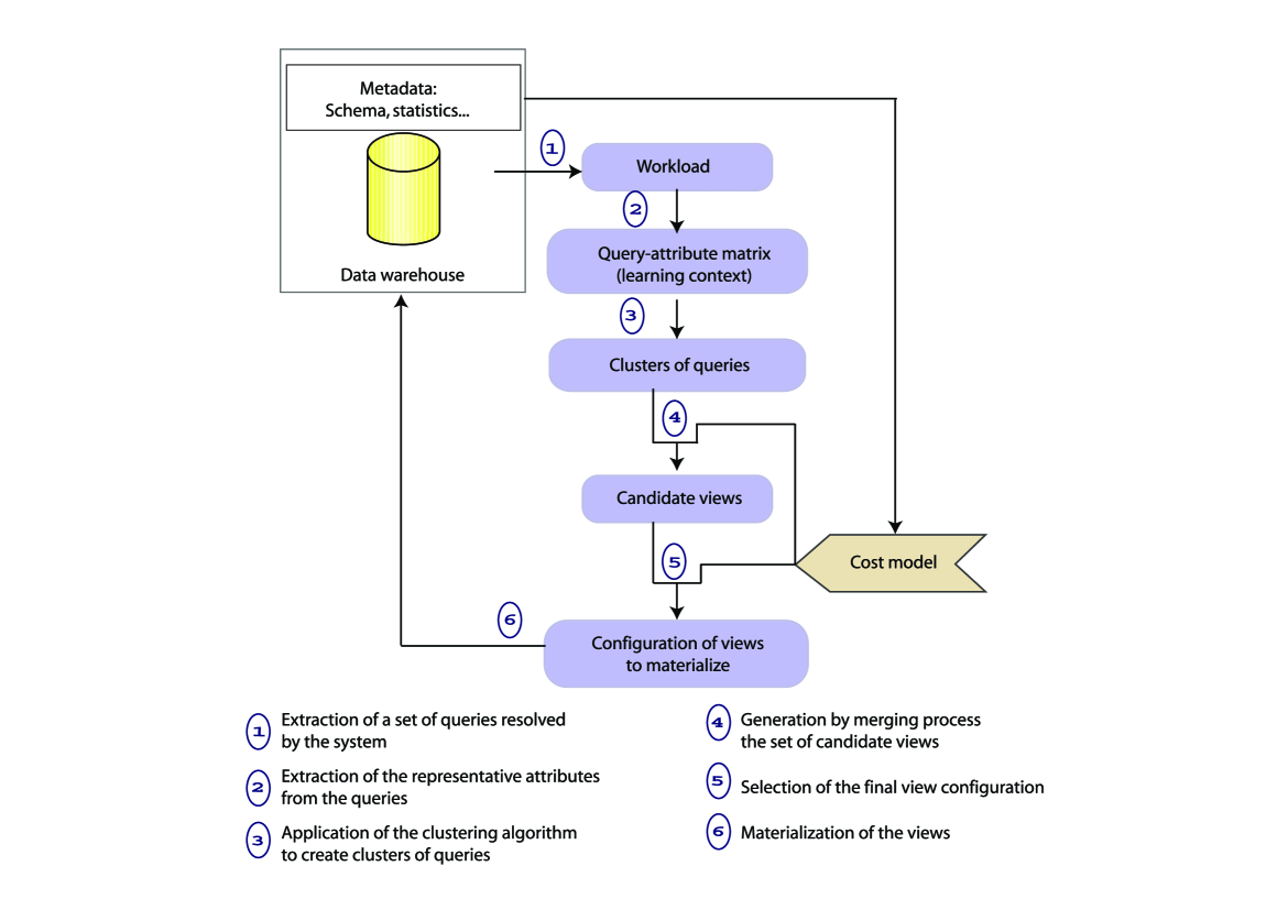
Figure 1: Strategy of materialized view selection

2.1 Query workload analysis

The workloads we consider are sets of GPSJ (Generalized Projection-Selection-Join) queries. A GPSJ query $q$ is composed of joins, selection predicates and aggregations. As such, it may be expressed in relational algebra over a star schema as follows: $q=\pi_{G,M}\sigma_{S}(F\bowtie D_{1}\bowtie D_{2}\bowtie\dots\bowtie D_{d})$, where $S$ is a conjunction of simple range predicates on dimension table attributes, $G$ is a set of attributes from dimension tables $D_{i}$ (grouping set), and $M$ is a set of aggregated measures each defined by applying aggregation operator to a measure in fact table $F$. For example, query $q_{1}$ in Figure 3 may be expressed as follows: $q_{1}=\pi_{sales.time\_id,sum(quantity\_sold)}\sigma_{fiscal\_day=2}(sales\bowtie times)$.

The first step consists in extracting from the workload the attributes that are representative of each query. We mean by representative attributes those that are present in Where (join and selection predicate attributes) and Group by clauses. We also save for each query their aggregation operators and joined tables. A query $q_{i}$ is then seen as a line in a matrix composed of cells that correspond to the representative attributes. The general term $q_{ij}$ of this matrix is set to 1 if the extracted attribute is present in the query and to 0 otherwise. This matrix represents our clustering context. Moreover, we store in an appendix matrix the existing associations between the join attributes and queries, in the same manner. We illustrate this step by an example: from the workload shown in Figure 3, we build the clustering context depicted in Figure 3.

($q_{1}$)	select sales.time_id, sum(quantity_sold) from sales, times
	where sales.time_id = times.time_id and times.fiscal_day = 2
	group by sales.time_id;
($q_{2}$)	select sales.prod_id, sum(amount_sold) from sales, products, promotions
	where sales.prod_id = products.prod_id and sales.promo_id = promotions.promo_id and promotions.promo_category = ‘newspaper’
	group by sales.prod_id;
($q_{3}$)	select sales.cust_id, sum(amount_sold) from sales, customers, products, times
	where sales.cust_id = customers.cust_id and sales.prod_id = products.prod_id and sales.time_id = times.time_id and times.fiscal_day = 3 and customers.cust_marital_status =‘single’ and products.prod_category =‘Women’
	group by sales.cust_id;
…

Figure 2: Example of workload

	$a_{1}$	$a_{2}$	$a_{3}$	$a_{4}$	$a_{5}$	$a_{6}$	$a_{7}$	$a_{8}$	$a_{9}$	$a_{10}$	$a_{11}$	$a_{12}$		$a_{1}$ times.time_id	$a_{2}$ times.fiscal_day
$q_{1}$	1	1	1	0	0	0	0	0	0	0	0	0		$a_{3}$ sales.time_id	$a_{4}$ products.prod_id
$q_{2}$	0	0	0	1	0	1	1	1	1	0	0	0		$a_{5}$ products.prod_category	$a_{6}$ sales.promo_id
$q_{3}$	0	0	0	1	0	1	1	1	1	1	1	1		$a_{7}$ promotions.promo_id	$a_{8}$ sales.prod_id
$..$														$a_{9}$ promotions.promo_category	$a_{10}$ sales.cust_id
$..$														$a_{11}$ customers.cust_marital_status	$a_{12}$ customers.cust_id

Figure 3: Example of clustering context

2.2 Building the candidate view set

In practice, it is hard to search all the views that are syntactically relevant (candidate views) from the workload queries, because the search space is very large [1]. To reduce the size of this space, we propose to cluster the queries. Indeed, we group in a same cluster all the queries that are closely similar. Closely similar queries are queries having a close binary representation in the query-attribute matrix. Two closely similar queries can be resolved by using only one materialized view. Used within a clustering process, the similarity and dissimilarity measures defined in the next section ensures that queries within the same cluster strongly relate to each other whereas queries from different clusters are significantly distant to each other.

2.2.1 Similarity measure.

Let $QA$ be a query-attribute matrix that has a set of queries $Q=\{q_{i},i=1..n\}$ as rows and a set of attributes $A=\{a_{j},j=1..p\}$ as columns. The value $q_{ij}$ is equal to 1 if attribute $a_{j}$ is extracted from query $q_{i}$. Otherwise, $q_{ij}$ is equal to 0. We describe query $q_{i}$ by a vector of $p$ values $q_{i}=[q_{i1},...,q_{ip}]$. These $p$ values describe respectively the presence ($q_{ij}=1$) or absence ($q_{ij}=0$) of attribute $a_{j}$. This description model helps comparing two queries. Then, for example, we can consider queries $q_{1}$ and $q_{2}$ as closely similar if vectors $[q_{11},...,q_{1p}]$ and $[q_{21},...,q_{2p}]$ have the majority of their cells equal. This introduces the notion similarity and dissimilarity between queries.

2.2.2 Similarity and dissimilarity between queries.

We define the notion of similarity and dissimilarity between queries by two functions $\delta_{sim_{j}}(q_{k},q_{l})$ and $\delta_{dissim_{j}}(q_{k},q_{l})$ that measure the similarity between two queries $q_{k}$ and $q_{l}$ with respect to attribute $a_{j}$.

$$\delta_{sim_{j}}(q_{k},q_{l})=\left\{\begin{tabular}[]{l}$1$ if $q_{kj}=q_{lj}=1$\\ $0$ otherwise\end{tabular}\right.$$

This first function defines the notion of similarity between $q_{k}$ and $q_{l}$ following attribute $a_{j}$: two queries $q_{k}$ and $q_{l}$ are considered similar regarding attribute $a_{j}$ if and only if $q_{kj}=q_{lj}=1$, i.e., attribute $a_{j}$ is extracted from both queries.

$$\delta_{dissim_{j}}(q_{k},q_{l})=\left\{\begin{tabular}[]{l}$0$ if $q_{kj}=q_{lj}$\\ $1$ if $q_{kj}\neq q_{lj}$\end{tabular}\right.$$

This second function defines the notion of dissimilarity between queries $q_{k}$ and $q_{l}$ according to attribute $a_{j}$: two queries $q_{k}$ and $q_{l}$ are considered dissimilar according to attribute $a_{j}$ if only and if $q_{kj}\neq q_{lj}$, i.e., if one and only one of the queries does not contain $a_{j}$. Note that there is not a complete symmetry between the notion of similarity and dissimilarity: non similar queries according to an attribute are not necessarily dissimilar according to this attribute. For example, let $q_{1}$ and $q_{2}$ be queries such that $q_{1j}=0$ and $q_{2j}=0$, respectively. Then we have $\delta_{sim_{j}}(q_{1},q_{2})=0$ ($q_{1}$ and $q_{2}$ are not considered similar) and $\delta_{dissim_{j}}(q_{1},q_{2})=0$ ($q_{1}$ and $q_{2}$ are not considered dissimilar). This absence of full symmetry underlines the fact that the absence of the same attribute in two queries does not give an element of similarity or dissimilarity between these queries.

These measures can be extended to an attribute set $A=\{a_{1},\dots,a_{p}\}$ such that we get the degree of global similarity and dissimilarity between two queries: $sim(q_{k},q_{l})=\sum_{j=1}^{p}\delta_{sim_{j}}(q_{k},q_{l})$ and $dissim(q_{k},q_{l})=\sum_{j=1}^{p}\delta_{dissim_{j}}(q_{k},q_{l})$, where $0\leq sim(q_{k},$ $q_{l})\leq p$ and $0\leq dissim(q_{k},q_{l})\leq p$. Hence, the closer $sim(q_{a},q_{b})$ (resp. $dissim(q_{a},$ $q_{b})$) is to $p$ the more $q_{a}$ and $q_{b}$ can be considered globally similar (resp. dissimilar).

2.2.3 Similarity and dissimilarity between query sets.

As we do for two queries, we introduce two functions that take into account the degree of similarity and dissimilarity between two query sets. A set of queries (subset of $Q$) is denoted $C_{a}$. In order to translate the level of similarity (resp. dissimilarity) between query sets, we use function $Sim(C_{a},C_{b})$ (resp.     $Dissim(C_{i},C_{j})$) that determines the number of similarities (resp. dissimilarities) between two different sets of queries $C_{a}$ and $C_{b}$ ($C_{a}\neq C_{b}$):

$$Sim(C_{a},C_{b})=\sum_{q_{k}\in C_{a},q_{l}\in C_{b}}sim(q_{k},q_{l})$$

$$Dissim(C_{a},C_{b})=\sum_{q_{k}\in C_{a},q_{l}\in C_{b}}dissim(q_{k},q_{l})$$

where $0\leq Sim(C_{a},C_{b})\leq card(C_{a})\times card(C_{b})\times p$ and $0\leq Dissim(C_{a},C_{b})\leq card(C_{a})\times card(C_{b})\times p$. Hence, the closer $Sim(C_{a},C_{b})$ (resp. $Dissim(C_{a},C_{b})$) is to $card(C_{a})\times card(C_{b})\times p$ the more $C_{a}$ and $C_{b}$ can be considered similar (resp. dissimilar).

2.2.4 Similarity and dissimilarity within a query set.

The notion of similarity (resp. dissimilarity) within a query set corresponds to the number of similarities (resp. dissimilarities) between queries of a same set $C_{a}$. It consists of an extension of the similarity and dissimilarity functions defined between query sets: $Sim(C_{a})=\sum_{q_{k}\in C_{a},q_{l}\in C_{a},k<l}sim(q_{k},q_{l})\textrm{ and }Dissim(C_{a})=\sum_{q_{k}\in C_{a},q_{l}\in C_{a},k<l}dissim(q_{k},q_{l})$, where $0\leq Sim(C_{a})\leq\frac{card(C_{a})\times(card(C_{a})-1)\times p}{2}$ and $0\leq Dissim(C_{a})\leq\frac{card(C_{a})\times(card(C_{a})-1)\times p}{2}$. Hence, the close $Sim(C_{a})$ (resp. $Dissim(C_{a})$) is to $\frac{card(C_{a})\times(card(C_{a})-1)\times p}{2}$ the more $C_{a}$ contains queries that are globally similar (resp. dissimilar).

2.2.5 Query clustering.

Clustering involves the determination of groups of objects (here: queries) that reveal the the internal structure of data. These groups must be such as they are composed of objects with high similarity and objects from different clusters present a high dissimilarity.

Let us consider clustering $P_{h}$ of a query set, a quality measure of this clustering can be built as follows:

$$Q(P_{h}) = \sum_{\begin{tabular}[]{c}a=1..z,\\ b=1..z,a $<$ b\\ \end{tabular}}Sim(C_{a},C_{b})+\sum_{a=1}^{z}Dissim(C_{a})$$

$0\leq Q(P_{h})\leq\sum_{i=1..z,j=1..z,i<j}card(C_{i})\times card(C_{j})\times p+\sum_{i=1}^{z}\frac{card(C_{i})\times(card(C_{i})-1)\times p}{2}$

This measure permits to capture the natural aspect of a clustering. Hence, $Q(P_{h})$ measures simultaneously similarities between queries within the same cluster and dissimilarities between queries within different clusters. Thus, $Q(P_{h})$ evaluates simultaneously the homogeneity of clusters as well as the heterogeneity between clusters. Therefore, the clustering presenting a high intra-cluster homogeneity and a high inter-cluster disparity has a weak value of $Q(P_{h})$ and thereby appears as the most natural.

Jouve and Nicoloyannis proposed such a solution in the Kerouac clustering algorithm and its associated clustering quality measure [12]. We have chosen this algorithm because it has several interesting properties: (1) its computational complexity is relatively low (log linear regarding the number of queries and linear regarding the number of attributes) ; (2) it can deal with a high number of objects (queries) ; (3) it can deal with distributed data [13].

3 View merging process

If we materialize all the different views derived from the query clusters obtained in the previous step, we can obtain a high number of materialized views, especially if the number of queries within the workload is high. A view configuration obtained this way would not be very relevant if the storage space allotted by the data warehouse administrator was limited. Instead of materializing each view, it is better to only materialize views that can be used to resolve multiple queries. To solve this problem, we must enumerate the space of views that can be merged, determine how to guide the merging process, and finally build the set of merged views. View merging is relevant if the queries are strongly similar. As we cluster together closely similar queries, it is logical to apply the merging process on the set of queries present in each cluster. This significantly reduces the number of possible combinations when merging views. We detail in the following sections how we merge two views and then generalize this process to many views.

Merging of view couples. The merging of two views must ensure these conditions: (1) all queries resolved by each view must also be resolved by the merged view, and (2) the cost of using the couple of views must not be significatively greater than the cost obtained when using the merged view. Let $v_{1}$ and $v_{2}$ be a couple of views of the same cluster and $s_{11},\dots,s_{1m}$ the selection predicates that are in $v_{1}$ and not in $v_{2}$. In a dual way, let $s_{21},\dots,s_{1n}$ be the selection conditions present in $v_{2}$ and not in $v_{1}$. Merged view $v_{12}$ is obtained by applying Algorithm 1.

Algorithm 1 Merge_View_Pair$(v_{1},v_{2}$) 1: put $v_{1}$ and $v_{2}$ aggregation operations in $v_{12}$ operation aggregations 2: put the union of projection and group by attributes $v_{1}$ and $v_{2}$ in projection and group by clause of $v_{12}$ 3: put all attributes $s_{11},\dots,s_{1m}$ and $s_{21},\dots,s_{1n}$ in the group by clause of $v_{12}$ 4: put the selection predicates shared between $v_{1}$ and $v_{2}$ in the selection predicate clause of $v_{12}$      Algorithm 2 Mergin_View_Generation 1: $M=V_{1}$ 2: for ($k=2$; $V_{k-1}\neq\emptyset$; $k++$) do 3:    $C_{k}=$ View_Gen($V_{k-1}$) 4:    $M\leftarrow M\cup C_{k}$ 5:    for all (view $v\in M$) do 6:      Remove the parents of $v$ from $M$ 7:    end for 8: end for 9: return $M$

The merging of two views $v_{1}$ and $v_{2}$ is effective if $cost(v_{12})\geq((cost(v_{1})+cost(v_{2}))*x)$. Cost computation is detailed in Section 4. The value of $x$ is fixed empirically by the administrator. If it is small (resp. high), we privilege (resp. disadvantage) view merging.

Property 1

The view obtained by merging views $v_{1}$ and $v_{2}$ is the smallest view that resolves the query resolved by both $v_{1}$ and $v_{2}$.

Proof

To show that the view obtained by merging views $v_{1}$ and $v_{2}$ is the smallest view, we have to show that there is no view $v^{\prime}_{12}$ such as the data within $v^{\prime}_{12}$ are also included within $v_{12}$. We denote respectively views $v_{1}$, $v_{2}$ and $v_{12}$ $\pi_{G_{1},M_{1}}\sigma_{S_{1}}(F\bowtie\dots)$, $\pi_{G_{2},M_{2}}\sigma_{S_{2}}(F\bowtie\dots)$ and $\pi_{G_{12},M_{12}}\sigma_{S_{12}}(F\bowtie\dots)$, respectively, where:
– $G_{1}$, $G_{2}$ are respectively the attribute set of the group by clause of views $v_{1}$ and $v_{2}$;
– $S_{1}$, $S_{2}$ are respectively the attribute set of the selection predicates of $v_{1}$ and $v_{2}$;
– $G_{12}=G_{1}\cup G_{2}\cup(S_{1}\cup S_{2}-S_{1}\cap S_{2})$ is the attribute set of the group by clause of merged view $v_{12}$;
– $S_{12}=S_{1}\cap S_{2}$ is the set of attribute selection predicates within merged view $v_{12}$.

Note that sets $G_{12}$ and $S_{12}$ are obtained by applying lines 1 and 2 of Algorithm 1. Let us now assume that the data in view $v^{\prime}_{12}$, denoted $\pi_{G^{\prime}_{12},M^{\prime}_{12}}\sigma_{S^{\prime}_{12}}(F\bowtie\dots)$ are all in $v_{12}$. This means that both of the following conditions hold: (1) $G_{12}\subset G^{\prime}_{12}$, (2) $S_{12}\supset S^{\prime}_{12}$.

From the first condition, there is at least one attribute $x$ such that $x\in G^{\prime}_{12}$ and $x\notin G_{12}$. As we have $x\notin G_{12}$, then $x\notin G_{1}$, $x\notin G_{2}$ and $x\notin S_{1}\cup(S_{2}-S_{1}\cap S_{2})$ because $G_{12}=G_{1}\cup G_{2}\cup(S_{1}\cup S_{2}-S_{1}\cap S_{2})$. As $x\notin G_{1}$ and $x\notin G_{2}$, then $x$ is not in any clause of $v_{2}$. This means that $x\notin G^{\prime}_{12}$, which contradicts condition $x\in G^{\prime}_{12}$.

From the second condition, there is at least one attribute $y$ such that $y\in S_{12}$ and $y\notin S^{\prime}_{12}$. As we have $y\in S_{12}$, then $y\in S_{1}$ and $y\in S_{2}$ because $S_{12}=S_{1}\cup S_{2}$. As $y\in S_{1}$ and $y\in S_{2}$, then $y$ must be in all the predicates of the views obtained by merging $v_{1}$ and $v_{2}$. This means that $y\in S^{\prime}_{12}$, which contradicts condition $y\notin S^{\prime}_{12}$.

Merged view generation algorithm. The algorithm of view generation by merging is similar to algorithms searching for frequent itemsets. A frequent itemset lattice looks like a lattice of views within a given cluster. The lattice nodes represent the space of views obtained by merging.

Algorithm 3 Function View_Gen($V_{k-1})$ 1: $C_{k}=\emptyset$ 2: for all (view $v\in V_{k-1}$) do 3:    for all (view $u\in V_{k-1}$) do 4:      if ($v[1]=u[1]\wedge\dots\wedge v[k-2]=u[k-2]\wedge v[k-1]<u[k-1]$) then 5:        $c=$ Merge_View_Pair ($v$,$u$) 6:        if ($cost(c)\geq((cost(v)+cost(u))*x)$) then 7:          $C_{k}=C_{k}\cup\{c\}$   8:        end if 9:      end if 10:    end for 11: end for 12: return $C_{k}$      Algorithm 4
View_Configuration_Construction 1: $S\leftarrow\emptyset$ 2: repeat 3:    $v_{max}\leftarrow\emptyset$ 4:    $F_{max}\leftarrow 0$ 5:    for all $v_{j}\in V-S$ do 6:      if $F_{/S}(v_{j})>F_{max}$ then 7:        $F_{max}\leftarrow F_{/S}(v_{j})$ 8:        $v_{max}\leftarrow v_{j}$ 9:      end if 10:    end for 11:    if $F_{/S}(v_{max})>0$ then 12:      $S\leftarrow S\cup\{v_{max}\}$ 13:    end if 14: until ($F_{/S}(v_{max})\leq 0$ or $V-S=\emptyset$)

The algorithm of view generation by merging (Algorithm 3) uses an iterative approach by level to generate a new view. It explores the view lattice in breadth first. The input of the algorithm is $V_{1}$, a set of candidate views extracted from a given cluster. This algorithm outputs a set of candidate views obtained by merging. In the $k^{th}$ iteration, view set $V_{k-1}$ obtained by merging the $k-1^{th}$ level’s views from the lattice (computed in the last step) is used to generate the set $C_{k}$ of $k$-candidate views. This set is added to set $M$ (line 4). The parents of each view obtained by merging are then removed from set $M$ (lines 5 to 7).

The function for view generation by merging View_Gen($V_{k-1}$), called on line 3, takes as argument $V_{k-1}$ and returns $C_{k}$. Two views $v$ and $u$ within $V_{k-1}$ form a $k$-view $c$ if and only if they have ($k-2$) views in common. This is expressed using a lexicographic order in the condition of line 3. We denote by $v[1]\dots v[k-2]v[k-1]$ the merged views in the $k^{th}$ iteration that are used to derive $v$. Function Merge_View_Pair($v$,$u$) (Algorithm 1) called on line 5 of View_Gen generates a new view $c$. The condition of line 6 ensures, after generating a $k$-view from two $k-1$-views, that the candidate view does not have a cost greater than the cost of its parents.

4 Cost models

The number of candidate views is generally as high as the input workload is large. Thus, it is not feasible to materialize all the proposed views because of storage space constraints. To circumvent these limitations, we use cost models allowing to conserve only the most pertinent views. In most data warehouse cost models [8], the cost of a query $q$ is assumed to be proportional to the number of tuples in the view on which $q$ is executed. In the following section, we detail the cost model that estimates the size of a given view.

Let $ms(F)$ be the maximum size of fact table $F$, $|F|$ be the number of tuples in $F$, $D_{i}\_ID$ be a primary key of dimension $D_{i}$, $|D_{i}\_ID|$ be the cardinality of the attribute(s) that form the primary key, and $N$ be the number of dimension tables. Then, $ms(F)=\prod_{i=1}^{N}|D_{i}\_ID|$.

Let $ms(V)$ be the maximum size of a given view $v$ that has attributes $a_{1},a_{2},\dots,a_{k}$ in its group by clause, where $k$ is the number of attributes in $v$ and $|a_{i}|$ is the cardinality of attribute $a_{i}$. Then, $ms(v)=\prod_{i=1}^{k}|a_{i}|$.

Golfarelli et al. [8] proposed to estimate the number of tuples in a given view $v$ by using Yao’s formula [24] as follows:
$|v|=ms(v)\times\left[1-\prod_{i=1}^{|F|}\frac{ms(F)\times d-i+1}{ms(F)-i+1}\right],\textrm{where }d=1-\frac{1}{ms(v)}.$ If $\frac{ms(F)}{ms(v)}$ is sufficiently large, then Cardenas’ formula [4] approximation gives:
$|v|=ms(v)\times\left(1-\left(1-\frac{1}{ms(v)}\right)^{|F|}\right),\textrm{where }d=1-\frac{1}{ms(v)}.$

Cardenas’ and Yao’s formulaes are based on the assumption that data is uniformly distributed. Any skew in the data tends to reduce the number of tuples in the aggregate view. Hence, the uniform assumption tends to overestimate the size of the views and give a crude estimation. However, they have the advantage to be simple to implement and fast to compute. In addition, because of the modularity of our approach, it is easy to replace the cost model module by another more accurate one.

From the number of tuples in $v$, we estimate its size, in bytes, as follows: $size(v)=|v|\times\sum_{i=1}^{c}size(c_{i})$, where $size(c_{i})$ denotes the size, in bytes, of column $c_{i}$ of $v$, and $c$ is the number of columns in $v$.

5 Objective functions

In this section, we describe three objective functions to evaluate the variation of query execution cost, in number of tuples to read, induced by adding a new view. The query execution cost is assimilated to the number of tuples in the fact table when no view is used or to the number of tuples in view(s) otherwise. The workload execution cost is obtained by adding all execution costs for each query within this workload.

The first objective function advantages the views providing more profit while executing queries, the second one advantages the views providing more benefit and occupying the smallest storage space, and the third one combines the first two in order to select at first all the views providing more profit and then keep only those occupying the smallest storage space when this resource becomes critical. The first function is useful when storage space is not limited, the second one is useful when storage space is small and the third one is interesting when storage space is larger.

5.1 Profit objective function

Let $V=\{v_{1},...,v_{m}\}$ be a candidate view set, $Q=\{q_{1},...,q_{n}\}$ a query set (a workload) and $S$ a final view set to build. The profit objective function, noted $P$, is defined as follows:
$P_{/S}(v_{j})=\left(C_{/S}(Q)-C_{/S\cup\{v_{j}\}}(Q)-\beta\>C_{maintenance}({\{v_{j}\}})\right)$, where ${v}_{j}\notin S$.

• $C_{/S}(Q)$ denotes the query execution cost when all views in $S$ are used. If this set is empty, $C_{/\emptyset}(Q)=|Q|\times|F|$ because all the queries are resolved by accessing fact table $|F|$. When a view $v_{j}$ is added to $S$, $C_{/S\cup\{v_{j}\}}(Q)=\sum_{k=0}^{|Q|}C(q_{k},\{v_{j}\})$ denotes the query execution cost for the views that are in $S\cup\{v_{j}\}$. If query $q_{k}$ exploits $v_{j}$, the cost $C(q_{k},\{v_{j}\})$ is then equal to $C_{v_{j}}$ (number of tuples in $v_{j}$). Otherwise, $C(q_{k},\{v_{j}\})$ is equal to the minimum value between $|F|$ and values of $C(q_{k},\{v\})$ (executing cost of $q_{k}$ exploiting $v\in S$ with $v\neq v_{j}$).
  

• Coefficient $\beta=|Q|\>p(v_{j})$ estimates the number of updates for view $v_{j}$. The update probability $p(v_{j})$ is equal to $\frac{1}{number\>of\>views}\frac{\%update}{\%query}$, where $\frac{\%update}{\%query}$ represents the proportion of updating vs. querying the data warehouse.
  

• $C_{maintenance}(\{v_{j}\})$ represents the maintenance cost for view $v_{j}$.

5.2 Profit/space ratio objective function

If view selection is achieved under a space constraint, the profit/space objective function $R_{/S}(v_{j})=\frac{P_{/S}(v_{j})}{size(v_{j})}$ is used. This function computes the profit provided by $v_{j}$ in regard to the storage space $size(v_{j})$ that it occupies.

5.3 Hybrid objective function

The constraint on the storage space may be relaxed if this space is relatively large. The hybrid objective function $H$ does not penalize space–“greedy” views if the ratio $\frac{remaining\_space}{storage\_space}$ is lower or equal than a given threshold $\alpha$ ($0<\alpha\leq 1$), where $remaining\_space$ and $storage\_space$ are respectively the remaining space after adding $v_{j}$ and the allotted space needed for storing all the views. This function is computed by combining the two functions $P$ and $R$ as follows:

$H_{/S}(v_{j})=\left\{\begin{tabular}[]{ll}$P_{/S}(v_{j})$&if $\frac{remaining\_space}{storage\_space}>\alpha$,\\ $R_{/S}(v_{j})$&otherwise.\\ \end{tabular}\right.$

6 View selection algorithm

The view selection algorithm (Algorithm 4) is based on a greedy search within the candidate view set $V$. Objective function $F$ must be one of the functions $P$ or $R$ described previously. If $R$ is used, we add to the algorithm’s input the space storage $M$ allotted for views.

In the first algorithm iteration, the values of the objective function are computed for each view within $V$. The view $v_{max}$ that maximizes $F$, if it exists ($F_{/S}(v_{max})>0$), is then added to $S$. If $R$ is used, the whole space storage $M$ is decreased by the amount of space occupied by $v_{max}$.

The function values of $F$ are then recomputed for each remaining view in $V-S$ since they depend on the selected views present in $S$. This helps taking into account the interactions that probably exist between the views.

We repeat these iterations until there is no improvement ($F_{/S}(v)\leq 0$) or until all views have been selected ($V-S=\emptyset$). If function $R$ is used, the algorithm also stops when storage space is full.

7 Experiments

In order to validate our approach for materialized view selection, we have run tests on a 1 GB data warehouse implemented within Oracle $9i$, on a Pentium 2.4 GHz PC with a 512 MB main memory and a 120 GB IDE disk. This data warehouse is composed of the fact table Sales and five dimensions Customers, Products, Times, Promotions and Channels. We executed on our data warehouse a workload composed of sixty-one decision-support queries involving aggregation operations and several joins between the fact table and dimension tables. Due to space constraints, the data warehouse schema and the detail of each workload query are available at http://eric.univ-lyon2.fr/~kaouiche/adbis.pdf. Our experiments are based on an ad-hoc benchmark because, as far as we know, there is no standard benchmark for data warehouses. TPC-R [21] has no multidimensional schema and does not qualify, for instance.

We first applied our selection strategy with the profit function. This function gives us the maximal number of materialized views (twelve views) because it does not specify any storage space constraint. This point gives us the upper boundary of the storage space occupation. Then, we applied the profit/space ratio and hybrid functions under a storage space constraint. We have measured query execution time with respect to the percentage of storage space allotted for materialized views. This percentage is computed from the upper boundary computed when applying the profit function. This helps varying storage space within a wider interval.

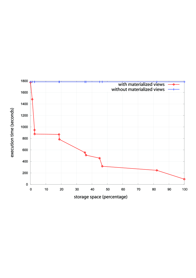
Figure 4: Profit/space ratio function

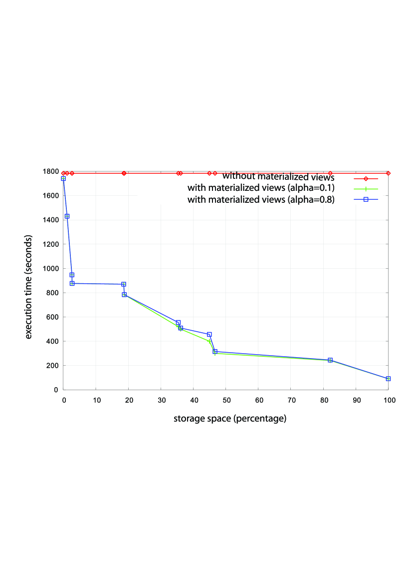
Figure 5: Hybrid function

7.0.1 Ratio profit/space function experiment.

We plotted in Figure 5 the variation of workload execution time with respect to the storage space allotted for materialized views. This figure shows that the selected views improve query execution time. Moreover, execution time decreases when storage space occupation increases. This is predictable because we create more materialized views when storage space is large and thereby better improve execution time. We also observe that the maximal gain is equal to $94.86\%$. It is reached for a space occupation of $100\%$ (no constraint on storage space). This case is also reached when using the profit function, because it corresponds to the upper boundary.

7.0.2 Hybrid function experiment.

We repeated the previous experiment with the hybrid objective function. We varied the value of parameter $\alpha$ between 0.1 and 1 by 0.1 steps. The obtained results with $\alpha\in[0.1,0.7]$ and $\alpha\in[0.8,1]$ are respectively equal to those obtained with $\alpha=0.1$ and $\alpha=0.8$. Thus, we plotted in Figure 5 only the results obtained with $\alpha=0.1$ and $\alpha=0.7$. This figure shows that for percentage values of space storage under 18.6%, the hybrid function with $\alpha=0.1$ and $\alpha=0.8$ behaves as the ratio function. When the storage space becomes critical, the hybrid function behaves as the ratio profit/space function. On the other hand, for the percentage values of storage space greater than 18.6%, the results obtained with $\alpha=0.8$ are slightly better than those obtained with $\alpha=0.1$. This is explained by the fact that for the high values of $\alpha$, the hybrid function chooses the views providing the most profit and thereby improving the best the execution time. The maximal gain in execution time observed for the values 0.1 and 0.8 of $\alpha$ is equal to $96\%$.

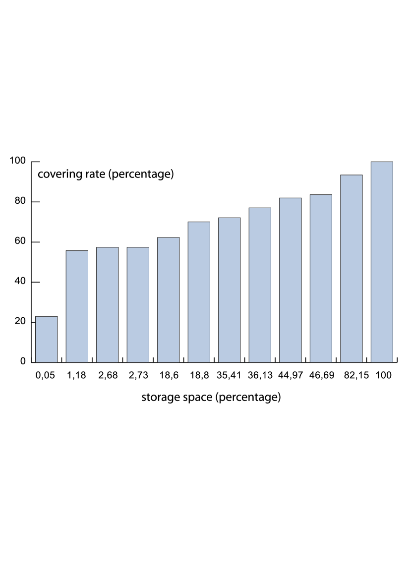
Figure 6: Query covering rate by the selected materialized views

7.0.3 Selected view pertinence experiment.

In order to show if our strategy provides pertinent views for a given workload, we measured the covering rate of the workload query results by the selected views. We mean by covering rate the ratio between the number of queries resolved from the materialized views and the total number of queries within the workload. Thus, the highest the rate value, the most pertinent the selected views. In this experiment, the percentage of storage space is also computed from the upper boundary. We plotted in Figure 6 the covering rate according to storage space occupation. This figure shows that the covering rate increases with storage space. When storage space gets larger, we materialize more views and thereby we recover more query results from these views. When materializing all the views (100% storage space occupation), all the data corresponding to query results are recovered from the materialized views. This shows that, without storage space constraint, the selected views are pertinent. For example, for 0.05% storage space occupation, 22.95% of the query results are recovered from the selected views. This shows that, even for a limited storage space, our strategy helps building views that cover a maximum number of queries. This experiment shows that materialized view selection based on workload syntactical analysis is efficient to guarantee the exploitation of the selected views by the workload queries.

8 Conclusion

In this paper, we presented an automatic strategy for materialized view selection in data warehouses. This strategy exploits the results of clustering applied on a given workload to build a set of syntactically relevant candidate views. Our experimental results show that our strategy guarantees a substantial gain in performance. It also shows that the idea of using data mining techniques for data warehouse auto-administration is a promising approach.

This work opens several future research axes. First, we are still currently experimenting in order to better evaluate system overhead in terms of materialized view building and maintenance. The maintenance cost is currently derived from the query frequencies (Section 4). We are envisaging a more accurate cost model to estimate update costs. We also plan to compare our approach to other materialized view selection methods. Furthermore, it could be interesting to design methods that select both indexes and materialized views, since these data structures are often used together. More precisely, we are currently developing methods to efficiently share the available storage space between indexes and views. Finally, our strategy is applied on a workload that is extracted from the system during a given period of time. We are thus performing static optimization. It would be interesting to make our strategy dynamic and incremental, as proposed in [14]. Studies dealing with dynamic or incremental clustering may be exploited. Entropy-based session detection could also be beneficial to determine the best moment to run view reselection.

References

- [1] S. Agrawal, S. Chaudhuri, and V. Narasayya. Automated selection of materialized views and indexes in SQL databases. In 26th International Conference on Very Large Data Bases (VLDB 2000), Cairo, Egypt, pages 496–505, 2000.
- [2] E. Baralis, S. Paraboschi, and E. Teniente. Materialized views selection in a multidimensional database. In 23rd International Conference on Very Large Data Bases (VLDB 1997), Athens, Greece, pages 156–165, 1997.
- [3] X. Baril and Z. Bellahsene. Selection of materialized views: a cost-based approach. In 15th International Conference (CAiSE 2003), Klagenfurt, Austria, pages 665–680, 2003.
- [4] A. F. Cardenas. Analysis and performance of inverted data base structures. Communication in ACM, 18(5):253–263, 1975.
- [5] G. K. Y. Chan, Q. Li, and L. Feng. Design and selection of materialized views in a data warehousing environment: a case study. In 2nd ACM international workshop on Data warehousing and OLAP (DOLAP 1999), Kansas City, USA, pages 42–47, 1999.
- [6] M. F. de Souza and M. C. Sampaio. Efficient materialization and use of views in data warehouses. SIGMOD Record, 28(1):78–83, 1999.
- [7] J. Goldstein and P. Larson. Optimizing queries using materialized views: a practical, scalable solution. In ACM SIGMOD international conference on Management of data (SIGMOD 2001), Santa Barbara, USA, pages 331–342, 2001.
- [8] M. Golfarelli and S. Rizzi. A methodological framework for data warehouse design. In 1st ACM international workshop on Data warehousing and OLAP (DOLAP 1998), New York, USA, pages 3–9, 1998.
- [9] H. Gupta. Selection of views to materialize in a data warehouse. In 6th International Conference on Database Theory (ICDT 1997), Delphi, Greece, pages 98–112, 1997.
- [10] H. Gupta and I. S. Mumick. Selection of views to materialize in a data warehouse. IEEE Transactions on Knowledge and Data Engineering, 17(1):24–43, 2005.
- [11] V. Harinarayan, A. Rajaraman, and J. D. Ullman. Implementing data cubes efficiently. In ACM SIGMOD International Conference on Management of data (SIGMOD 1996), Montreal, Canada, pages 205–216, 1996.
- [12] P. Jouve and N. Nicoloyannis. KEROUAC: an algorithm for clustering categorical data sets with practical advantages. In International Workshop on Data Mining for Actionable Knowledge (DMAK’2003, in conjunction with PAKDD03), 2003.
- [13] P. Jouve and N. Nicoloyannis. A new method for combining partitions, applications for distributed clustering. In International Workshop on Paralell and Distributed Machine Learning and Data Mining (ECML/PKDD03), pages 35–46, 2003.
- [14] Y. Kotidis and N. Roussopoulos. DynaMat: A dynamic view management system for data warehouses. In ACM SIGMOD International Conference on Management of Data, (SIGMOD 1999), Philadelphia, USA, pages 371–382, 1999.
- [15] T. P. Nadeau and T. J. Teorey. Achieving scalability in OLAP materialized view selection. In 5th ACM International Workshop on Data Warehousing and OLAP (DOLAP 2002), McLean, USA.
- [16] S. Rizzi and E. Saltarelli. View materialization vs. indexing: Balancing space constraints in data warehouse design. In 15th International Conference (CAiSE 2003), Klagenfurt, Austria, pages 502–519, 2003.
- [17] A. Shukla, P. Deshpande, and J. F. Naughton. Materialized view selection for multi-cube data models. In 7th International Conference on Extending DataBase Technology (EDBT 2000), Konstanz, Germany, pages 269–284, 2000.
- [18] Y. Sismanis, A. Deligiannakis, N. Roussopoulos, and Y. Kotidis. Dwarf: shrinking the petacube. In ACM SIGMOD International Conference on Management of Data (SIGMOD 2002), Madison, USA, pages 464–475, 2002.
- [19] J. R. Smith, C.-S. Li, and A. Jhingran. A wavelet framework for adapting data cube views for OLAP. IEEE Transactions on Knowledge and Data Engineering, 16(5):552–565, 2004.
- [20] D. Theodoratos and W. Xu. Constructing search spaces for materialized view selection. In 7th ACM international workshop on Data warehousing and OLAP (DOLAP 2004), Washington, USA.
- [21] Transaction Processing Council. TPC Benchmark R Standard Specification, 1999.
- [22] H. Uchiyama, K. Runapongsa, and T. J. Teorey. A progressive view materialization algorithm. In 2nd ACM International Workshop on Data warehousing and OLAP (DOLAP 1999), Kansas City, USA, pages 36–41, 1999.
- [23] S. R. Valluri, S. Vadapalli, and K. Karlapalem. View relevance driven materialized view selection in data warehousing environment. In 30th Australasian conference on Database technologies, Melbourne, Australia, pages 187–196, 2002.
- [24] S. B. Yao. Approximating block accesses in database organizations. Communication in ACM, 20(4):260–261, 1977.