Automatic Selection of Bitmap Join Indexes
in Data Warehouses

Abstract

The queries defined on data warehouses are complex and use several join operations that induce an expensive computational cost. This cost becomes even more prohibitive when queries access very large volumes of data. To improve response time, data warehouse administrators generally use indexing techniques such as star join indexes or bitmap join indexes. This task is nevertheless complex and fastidious. Our solution lies in the field of data warehouse auto-administration. In this framework, we propose an automatic index selection strategy. We exploit a data mining technique ; more precisely frequent itemset mining, in order to determine a set of candidate indexes from a given workload. Then, we propose several cost models allowing to create an index configuration composed by the indexes providing the best profit. These models evaluate the cost of accessing data using bitmap join indexes, and the cost of updating and storing these indexes.

1 Introduction

Data warehouses are generally modelled according to a star schema that contains a central, large fact table, and several dimension tables that describe the facts [10, 11]. The fact table contains the keys of the dimension tables (foreign keys) and measures. A decision–support query on this model needs one or more joins between the fact table and the dimension tables. These joins induce an expensive computational cost. This cost becomes even more prohibitive when queries access very large data volumes. It is thus crucial to reduce it.

Several database techniques have been proposed to improve the computational cost of joins, such as hash join, merge join and nested loop join [14]. However, these techniques are efficient only when a join applies on two tables and data volume is relatively small. When the number of joins is greater than two, they are ordered depending on the joined tables (join order problem). Other techniques, used in the data warehouse environment, exploit join indexes to pre-compute these joins in order to ensure fast data access. Data warehouse administrators then handle the crucial task of choosing the best indexes to create (index selection problem). This problem has been studied for many years in databases [1, 4, 5, 6, 7, 12, 18]. However, it remains largely unresolved in data warehouses. Existing research studies may be clustered in two families: algorithms that optimize maintenance cost [13] and algorithms that optimize query response time [2, 8, 9]. In both cases, optimization is realized under the constraint of the storage space. In this paper, we focus on the second family of solutions, which is relevant in our context because they aim to optimize query response time.

In addition, with the large scale usage of databases in general and data warehouses in particular, it is now very important to reduce the database administration function. The aim of auto-administrative systems is to administrate and adapt themselves automatically, without loss (or even with a gain) in performance. In this context, we proposed a method for index selection in databases based on frequent itemset extraction from a given workload [3]. In this paper, we present the follow-up of this work. Since all candidate indexes provided by the frequent itemset extraction phase cannot be built in practice due to system and storage space constraints, we propose a cost model–based strategy that selects the most advantageous indexes. Our cost models estimate the data access cost using bitmap join indexes, and their maintenance and storage cost.

We particularly focus on bitmap join indexes because they are well–adapted to data warehouses. Bitmap indexes indeed make the execution of several common operations such as And, Or, Not or Count efficient by having them operating on bitmaps, in memory, and not on the original data. Furthermore, joins are pre-computed at index creation time and not at query execution time. The storage space occupied by bitmaps is also low, especially when the indexed attribute cardinality is not high [17, 19]. Such attributes are frequently used in decision–support query clauses such as Where and Group by.

The remainder of this paper is organized as follows. We first remind the principle of our index selection method based on frequent itemset mining (Section 2). Then, we detail our cost models (Section 3) and our index selection strategy (Section 4). To validate our work, we also present some experiments (Section 5). We finally conclude and provide research perspectives (Section 6).

2 Index selection method

In this section, we present an extension to our work about the index selection problem [3]. The method we propose (Figure 1) exploits the transaction log (the set of all the queries processed by the system) to recommend an index configuration improving data access time.

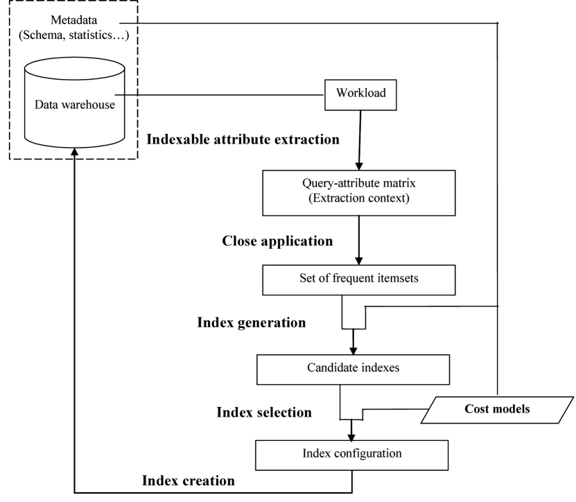
Figure 1: Automatic index selection strategy

We first extract from a given workload a set of so called indexable attributes. Then, we build a “query-attribute” matrix whose rows represent workload queries and whose columns represent a set of all the indexable attributes. Attribute presence in a query is symbolized by one, and absence by zero. It is then exploited by the Close frequent itemset mining algorithm [16]. Each itemset is analyzed to generate a set of candidate indexes. This is achieved by exploiting the data warehouse metadata (schema: primary keys, foreign keys; statistics…). Finally, we prune the candidate indexes using the cost models presented in Section 3, before effectively building a pertinent index configuration. We detail these steps in the following sections.

3 Cost models

The number of candidate indexes is generally as high as the input workload is large. Thus, it is not feasible to build all the proposed indexes because of system limits (limited number of indexes per table) or storage space constraints. To circumvent these limitations, we propose cost models allowing to conserve only the most advantageous indexes. These models estimate the storage space (in bytes) occupied by bitmap join indexes, the data access cost using these indexes and their maintenance cost expressed in number of input/output operations (I/Os). Table 1 summarizes the notations used in our cost models.

Table 1: Cost model parameters

Symbol	Description
$\mid X\mid$	Number of tuples in table X or cardinality of attribute X
$S_{p}$	Disk page size in bytes
$p_{X}$	Number of pages needed to store table X
$S_{pointer}$	Page pointer size in bytes
m	B-tree order
d	Number of bitmaps used to evaluate a given query
$w(X)$	Tuple size in bytes of table X or attribute X

3.1 Bitmap join index size

The space required to store a simple bitmap index linearly depends on the indexed attribute cardinality and the number of tuples in the table on which the index is built. The storage space of a bitmap index built on attribute $A$ from table $T$ is equal to $\frac{|A||T|}{8}$ bytes [19, 20]. Bitmap join indexes are built on dimension table attributes. Each bitmap contains as many bits as the number of tuples in fact table $F$. The size of their storage space is then $S=\frac{|A||F|}{8}$ bytes.

3.2 Bitmap join index maintenance cost

Data updates (mainly insert operations in decisions-support systems) systemically trigger index updates. These operations are applied either on a fact table or dimensions. The cost of updating bitmap join indexes is presented in the following sections.

Insertion cost in fact table. Assume a bitmap join index built on attribute $A$ from dimension table $T$. While inserting tuples in fact table $F$, it is first necessary to search for the tuple of $T$ that is able to be joined with them. At worst, the whole table $T$ is scanned ($P_{T}$ pages are read). It is then necessary to update all bitmaps. At worst, all bitmaps are scanned: $\frac{|A||F|}{8S_{p}}$ pages are read, where $S_{p}$ denotes the size of one disk page. The index maintenance cost is then $C_{maintenance}=p_{T}+\frac{|A||F|}{8S_{p}}$.

Insertion cost in dimension tables. An insertion in dimension $T$ may induce or not a domain expansion for attribute $A$. When not expanding the domain, the fact table is scanned to search for tuples that are able to be joined with the new tuple inserted in $T$. This operation requires to read $p_{F}$ pages. It is then necessary to update the bitmap index. This requires $\frac{|A||F|}{8S_{p}}$ I/Os. When expanding the domain, it is necessary to add the cost of building a new bitmap ($\frac{|F|}{8S_{p}}$ pages). The maintenance cost of bitmap join indexes is then $C_{maintenance}~{}=~{}p_{F}+(1+\xi)\frac{|A||F|}{8S_{p}}$, where $\xi$ is equal to one if there is expansion and zero otherwise.

3.3 Data access cost

We propose two cost models to estimate the number of I/Os needed for data access. In the first model, we do not take any hypothesis about how indexes are physically implemented. In the second model, we assume that access to the index bitmaps is achieved through a b-tree such as is the case in Oracle. Due to lack of space and our experiments under Oracle we only detail here the second model because of running our experiments. however, the first model is not detailed here due to the lack of space.

In this model, we assume that the access to bitmaps is realized through a b-tree (meta–indexing) in which leaf nodes point to bitmaps (appendix figure LABEL:fig:bitmap_join). The cost, in number of I/Os, of exploiting a bitmap join index for a given query may be written as follows: $C~{}=~{}C_{descent}~{}+~{}C_{scan}~{}+~{}C_{read}$, where $C_{descent}$ denotes the cost needed to reach the leaf nodes from the b-tree root, $C_{scan}$ denotes the cost of scanning leaf nodes to retrieve the right search key and the cost of reading the bitmaps associated to this key, and $C_{read}$ finally gives the cost of reading the indexed table’s tuples.

The descent cost in the b-tree depends on its height. The b-tree’s height built on attribute $A$ is $log_{m}|A|$, where $m$ is the b-tree’s order. This order is equal to $K+1$, where $K$ represents the number of search keys in each b-tree node. $K$ is equal to $\frac{S_{p}}{w(A)+S_{pointer}}$, where $w(A)$ and $S_{pointer}$ are respectively the size of the indexed attribute $A$ and the size of a disk page pointer in bytes. Without adding the b-tree leaf node level, the b-tree descent cost is then $C_{descent}=log_{m}|A|-1$.

The scanning cost of leaf nodes is $\frac{|A|}{m-1}$ (at worst, all leaf nodes are read). Data access is achieved through bits set to one in each bitmap. In this case, it is necessary to read each bitmap. The reading cost of $d$ bitmaps is $d\frac{|F|}{8S_{p}}$. Hence, the scanning cost of the leaf nodes is $C_{scan}=\frac{|A|}{m-1}+d\frac{|F|}{8S_{p}}$.

The reading cost of the indexed table’s tuples is computed as follow. For a bitmap index built on attribute $A$, the number of read tuples is equal to $\frac{|F|}{|A|}$ (if data are uniformly distributed). Generally, the total number of read tuples for a query using $d$ bitmaps is $N_{r}=d\frac{|F|}{|A|}$. Knowing the number of read tuples, the number of I/Os in the reading phase is $C_{read}=p_{F}(1-e^{-\frac{N_{r}}{p_{F}}})$ [15], where $p_{F}$ denotes the number of pages needed for store the fact table.

In summary, the evaluation cost of a query exploiting a bitmap join index is $C_{index}=log_{m}|A|-1+\frac{|A|}{m-1}+d\frac{|F|}{8S_{p}}+p_{F}(1-e^{-\frac{N_{r}}{p_{F}}})$.

3.4 Join cost without indexes

If the bitmap join indexes are not useful while evaluating a given query, we assume that all joins are achieved by the hash–join method. The number of I/Os needed for joining table $R$ with table $S$ is then $C_{hash}~{}=~{}3~{}(p_{S}~{}+~{}p_{R})$ [14].

4 Bitmap join index selection strategy

Our index selection strategy proceeds in several steps. The candidate index set is first built from the frequent itemsets mined from the workload (Section 2). A greedy algorithm then exploits an objective function based on our cost models (Section 3) to prune the least advantageous indexes. The detail of these steps and the construction of the objective function are provided in the following sections.

4.1 Candidate index set construction

From the frequent itemsets (Section 2) and the data warehouse schema (foreign keys of the fact table, primary keys of the dimensions, etc.), we build a set of candidate indexes.

The SQL statement for building a bitmap join index is composed of three clauses: On, From and Where. The On clause is composed of attributes on which is built the index (non–key attributes in the dimensions), the From clause contains all joined tables and the Where clause contains the join predicates.

We consider a frequent itemset $<Table.attribute_{1},...,Table.attribute_{n}>$ composed of elements such as $Table.attribute$. Each itemset is analyzed to determine the different clauses of the corresponding index. We first extract the elements containing foreign keys of the fact table because they are necessary to define the From and Where index clauses. Next, we retrieve the itemset elements that contain primary keys of dimensions to form the From index clause. The elements containing non–key attributes of dimensions form the On index clause. If such elements do not exist, the bitmap join index cannot be built.

4.2 Objective functions

In this section, we describe three objective functions to evaluate the variation of query execution cost, in number of I/Os, induced by adding a new index. The query execution cost is assimilated to computing the cost of hash joins if no bitmap join index is used or to the data access cost through indexes otherwise. The workload execution cost is obtained by adding all execution costs for each query within this workload. The first objective function advantages the indexes providing more profit while executing queries, the second one advantages the indexes providing more benefit and occupying less storage space, and the third one combines the first two in order to select at first all indexes providing more profit and then keep only those occupying less storage space when this resource becomes critical. The first function is useful when storage space is not limited, the second one is useful when storage space is small and the third one is interesting when this storage space is quite large. The detail of computing each function is not given due to the lack of space.

4.3 Index configuration construction

The index selection algorithm is based on a greedy search within the candidate index set $I$ given as an input. The objective function $F$ must be one of the functions: profit ($P$), profit/space ratio ($R$) or hybrid ($H$). If $R$ is used, we add to the algorithm’s input the space storage $M$ allotted for indexes. If $H$ is used, we also add threshold $\alpha$ as input.

In the first algorithm iteration, the values of the objective function are computed for each index within $I$. The execution cost of all queries in workload $Q$ is equal to the total cost of hash joins. The index $i_{max}$ that maximizes $F$, if it exists, is then added to the set of selected indexes $S$. If $R$ or $H$ is used, the whole space storage $M$ is decreased by the amount of space occupied by $i_{max}$.

The function values of $F$ are then recomputed for each remaining index in $I-S$ since they depend on the selected indexes present in $S$. This helps taking into account the interactions that probably exist between the indexes. We repeat these iterations until there is no improvement or all indexes have been selected ($I-S=\emptyset$). If functions $R$ or $H$ are used, the algorithm also stops when storage space is full.

5 Experiments

In order to validate our bitmap join index selection strategy, we have run tests on a data warehouse implemented within Oracle $9i$, on a Pentium 2.4 GHz PC with a 512 MB main memory and a 120 GB IDE disk. This data warehouse is composed of the fact table Sales and five dimensions Customers, Products, Promotions, Times and Channels. We have measured for different value of the minimal support parameterized in Close the workload execution time. In practice, the minimal support limits the number of candidate indexes to generate and selects only those that are frequently used.

For computing the different costs from our models, we fixed the value of $S_{p}$ (disk page size) and $S_{pointer}$ (page pointer size) to 8 MB and 4 MB respectively. These values are those indicated in the Oracle $9i$ configuration file. The workload is composed of forty decision–support queries containing several joins. We measured the total execution time when building indexes or not. In the case of building indexes, we also measured the total execution time when we applied each objective function among of profit, ratio profit/space and hybrid. We also measured the disk space occupied by the selected indexes. When applying the cost models, we reduce the number of indexes and thereby the storage space needed to store these indexes.

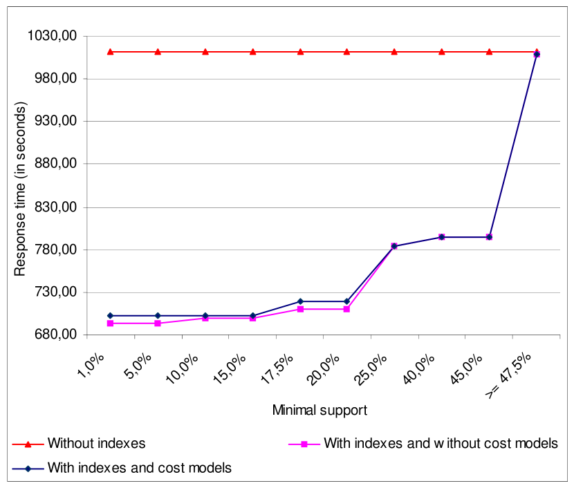
Figure 2: Profit function

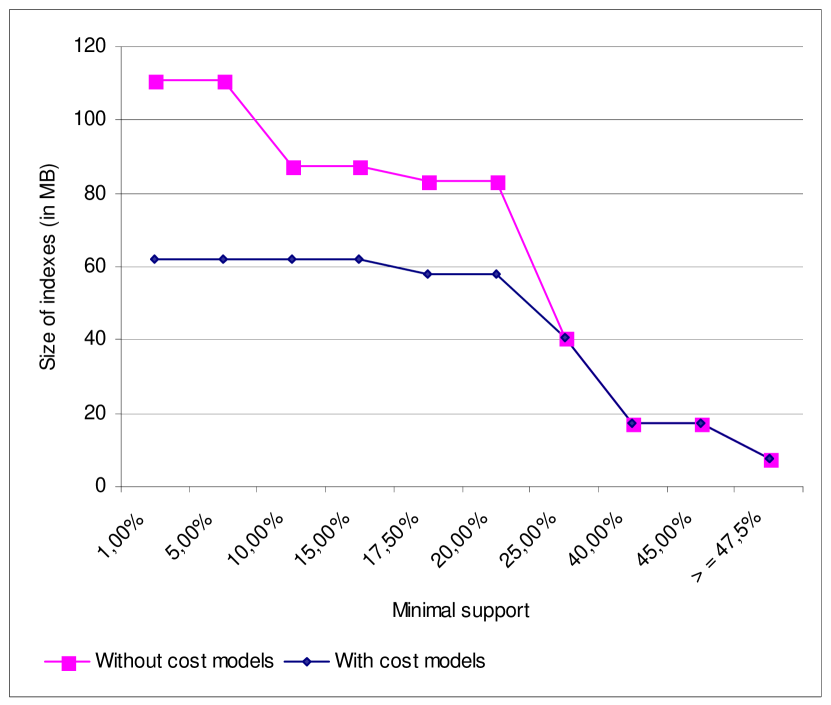
Figure 3: Index storage space

Profit function experiment. Figure 3 shows that the selected indexes improve query execution time with and without application of our cost models until the minimal support forming frequent itemsets reaches 47.5%. Moreover, the execution time decreases continuously when the minimal support increases because the number of indexes decreases. For high values of the minimal support (greater than 47.5%), the execution time is closer to the one obtained without indexes. This case is predictable because there is no or few candidate indexes to create. The maximal gain in time in both cases is respectively 30.50% and 31.85%. Despite of this light drop of 1.35% in time gain when the cost models are used (fewer indexes are built), we observe a significant gain in storage space (equal to 32.79% in the most favorable case) as shown in figure 3. This drop in number of indexes is interesting when the data warehouse update frequency is high because update time is proportional to the number of indexes. On the other hand, the gain in storage space helps limiting the storage space allotted for indexes by the administrator.

Profit/space ratio function experiment. In these experiments, we have fixed the value of minimal support to 1%. This value gives the highest number of frequent itemsets and consequently the highest number of candidate indexes. This helps varying storage space within a wider interval. We have measured query execution time according to the percentage of storage space allotted for indexes. This percentage is computed from the space occupied by all indexes. Figure 5 shows that execution time decreases when storage space occupation increases. This is predictable because we create more indexes and thus better improve the execution time. We also observe that the maximal time gain is equal to 28.95% and it is reached for a space occupation of 59.64%. This indicates that if we fix space storage to this value, we obtain a time gain close to the one obtained with the profit objective function (30.50%). This case is interesting when the administrator does not have enough space to store all the indexes.

Hybrid function experiment. We repeated the previous experiments with the hybrid objective function. We varied the value of parameter $\alpha$ between 0.1 and 1 by 0.1 steps. The obtained results with $\alpha\in[0.1,0.7]$ and $\alpha\in[0.8,1]$ are respectively equal to those obtained with $\alpha=0.1$ and $\alpha=0.7$. Thus, we represent in figure 5 only the results obtained with $\alpha=0.1$ and $\alpha=0.7$. This figure shows that for $\alpha=0.1$, the results are close to those obtained with profit/space ratio the function ; and for $\alpha=0.8$, they are close to those obtained with the profit function. The maximal gain in execution time is respectively equal to 28.95% and 29.95% for $\alpha=0.1$ and $\alpha=0.8$. We explain these results by the fact that bitmap join indexes built on several attributes need more storage space. However, as they pre–compute more joins, they better improve the execution time. The space storage allotted for indexes then fills up very quickly after a few iterations of the greedy algorithm. This explains why the parameter $\alpha$ does not significantly affect our algorithm and the experiment results.

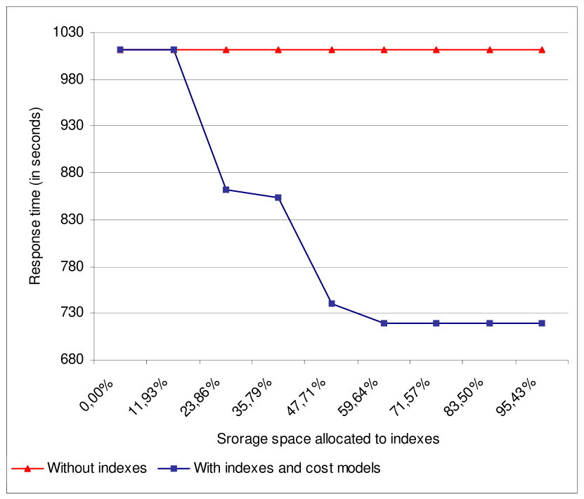
Figure 4: Profit/space ratio function

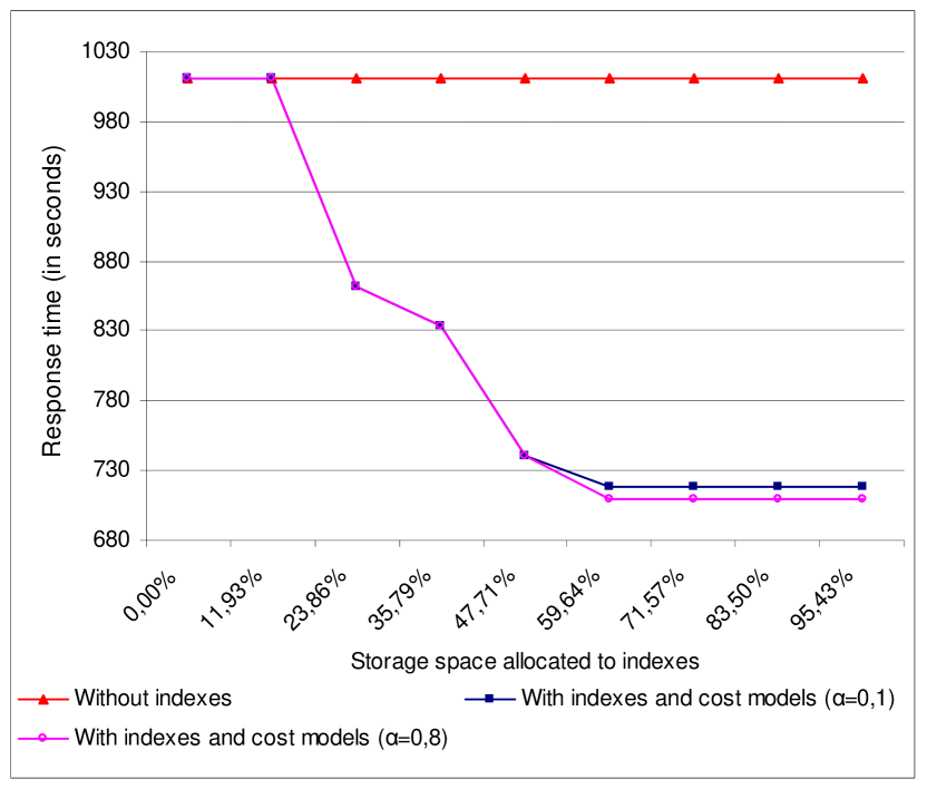
Figure 5: Hybrid function

6 Conclusion and perspectives

In this article, we presented an automatic strategy for bitmap index selection in data warehouses. This strategy first exploits frequent itemsets obtained by the Close algorithm from a given workload to build a set of candidate bitmap join indexes. With the help of cost models, we keep only the most advantageous candidate indexes. These models estimate data access cost through indexes, as well as maintenance and storage cost for these indexes. We have also proposed three objective functions: profit, profit/space ratio and hybrid that exploit our cost models to evaluate the execution cost of all queries. These functions are themselves exploited by a greedy algorithm that recommends a pertinent configuration of indexes. This helps our strategy respecting constraints imposed by the system (limited number of indexes per table) or the administrator (storage space allotted for indexes). Our experimental results show that the application of cost models to our index selection strategy decreases the number of selected indexes without a significant loss in performance. This decrease actually guarantees a substantial gain in storage space, and thus a decrease in maintenance cost during data warehouse updates.

Our work shows that the idea of using data mining techniques for data warehouse auto-administration is a promising approach. It opens several future research axes. First, it is essential to keep on experimenting in order to better evaluate system overhead in terms of index building and maintenance. It could also be very interesting to compare our approach to other index selection methods. Second, extending our approach to other performance optimization techniques (materialized views, buffering, physical clustering, etc.) is another promising perspective. Indeed, in a data warehouse environment, it is principally in conjunction with other physical structures such as materialized views that indexing techniques provide significant gains in performance. For example, our context extraction may be useful to build clusters of queries that maximize the similarity between queries within each cluster. Each cluster may be then a starting point to materialize views. In addition, it could be interesting to design methods to efficiently share the available storage space between indexes and views.

References

- [1] S. Agrawal, S. Chaudhuri, and V. Narasayya. Automated selection of materialized views and indexes in SQL databases. In 26th International Conference on Very Large Data Bases (VLDB 2000), Cairo, Egypt, pages 496–505, 2000.
- [2] S. Agrawal, S. Chaudhuri, and V. Narasayya. Materialized view and index selection tool for Microsoft SQL Server 2000. In ACM SIGMOD International Conference on Management of Data (SIGMOD 2001), Santa Barbara, USA, page 608, 2001.
- [3] K. Aouiche, J. Darmont, and L. Gruenwald. Frequent itemsets mining for database auto-administration. In 7th International Database Engineering and Application Symposium (IDEAS 2003), Hong Kong, China, pages 98–103, 2003.
- [4] S. Chaudhuri, M. Datar, and V. Narasayya. Index selection for databases: A hardness study and a principled heuristic solution. IEEE Transactions on Knowledge and Data Engineering, 16(11):1313–1323, 2004.
- [5] Y. Feldman and J. Reouven. A knowledge–based approach for index selection in relational databases. Expert System with Applications, 25(1):15–37, 2003.
- [6] S. Finkelstein, M. Schkolnick, and P. Tiberio. Physical database design for relational databases. ACM Transactions on Database Systems, 13(1):91–128, 1988.
- [7] M. Frank, E. Omiecinski, and S. Navathe. Adaptive and automated index selection in RDBMS. In 3rd International Conference on Extending Database Technology (EDBT 1992), Vienna, Austria, volume 580 of Lecture Notes in Computer Science, pages 277–292, 1992.
- [8] M. Golfarelli, S. Rizzi, and E. Saltarelli. Index selection for data warehousing. In 4th International Workshop on Design and Management of Data Warehouses (DMDW 2002), Toronto, Canada, pages 33–42, 2002.
- [9] H. Gupta, V. Harinarayan, A. Rajaraman, and J. D. Ullman. Index selection for OLAP. In 13th International Conference on Data Engineering (ICDE 1997), Birmingham, U.K., pages 208–219, 1997.
- [10] W. Inmon. Building the Data Warehouse. John Wiley & Sons, third edition, 2002.
- [11] R. Kimball and M. Ross. The Data Warehouse Toolkit: The Complete Guide to Dimensional Modeling. John Wiley & Sons, second edition, 2002.
- [12] J. Kratica, I. Ljubić, and D. Tošić. A genetic algorithm for the index selection problem. In Applications of Evolutionary Computing, Essex, England, volume 2611 of LNCS, pages 281–291, 2003.
- [13] W. Labio, D. Quass, and B. Adelberg. Physical database design for data warehouses. In 13th International Conference on Data Engineering (ICDE 1997), Birmingham, U.K., pages 277–288, 1997.
- [14] P. Mishra and M. Eich. Join processing in relational databases. ACM Computing Surveys, 24(1):63–113, 1992.
- [15] P. O’Neil and D. Quass. Improved query performance with variant indexes. In ACM SIGMOD International Conference on Management of Data (SIGMOD 1997), Tucson, USA, pages 38–49, 1997.
- [16] N. Pasquier, Y. Bastide, R. Taouil, and L. Lakhal. Discovering frequent closed itemsets for association rules. In 7th International Conference on Database Theory (ICDT 1999), Jerusalem, Israel, volume 1540 of LNCS, pages 398–416, 1999.
- [17] S. Sarawagi. Indexing OLAP data. Data Engineering Bulletin, 20(1):36–43, 1997.
- [18] G. Valentin, M. Zuliani, D. Zilio, G. Lohman, and A. Skelley. DB2 advisor: An optimizer smart enough to recommend its own indexes. In 16th International Conference on Data Engineering (ICDE 2000), San Diego, USA, pages 101–110, 2000.
- [19] M. Wu. Query optimization for selections using bitmaps. In ACM SIGMOD International Conference on Management of Data (SIGMOD 1999), Philadelphia, USA, pages 227–238, 1999.
- [20] M. Wu and A. Buchmann. Encoded bitmap indexing for data warehouses. In 14th International Conference on Data Engineering (ICDE 1998), Orlando, USA, pages 220–230, 1998.