AICA: a New Pair Force Evaluation Method for Parallel Molecular Dynamics in Arbitrary Geometries

Abstract

A new algorithm for calculating intermolecular pair forces in Molecular Dynamics (MD) simulations on a distributed parallel computer is presented. The Arbitrary Interacting Cells Algorithm (AICA) is designed to operate on geometrical domains defined by an unstructured, arbitrary polyhedral mesh, which has been spatially decomposed into irregular portions for parallelisation. It is intended for nano scale fluid mechanics simulation by MD in complex geometries, and to provide the MD component of a hybrid MD/continuum simulation. AICA has been implemented in the open-source computational toolbox OpenFOAM, and verified against a published MD code.

and

1 Introduction and Motivation

1.1 MD Simulation in Arbitrary Geometries

Simulations of nano scale liquid systems can provide insight into many naturally-occurring phenomena, such as the action of proteins that mediate water transport across biological cell membranes [1]. They may also facilitate the design of future nano devices and materials (e.g. high-throughput, highly selective filters or lab-on-a-chip components). The dynamics of these very small systems are dominated by surface interactions, due to their large surface area to volume ratios. However, these surface effects are often too complex and material-dependent to be treated by simple phenomenological parameters [2] or by adding ‘equivalent’ fluxes at the boundary [3]. Direct simulation of the fluid using molecular dynamics (MD) presents an opportunity to model these phenomena with minimal simplifying assumptions.

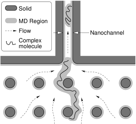
Figure 1: Schematic of an application of a hybrid MD/continuum simulation: complex molecules being transported into a nano channel. Only the complex molecules, regions near them and regions near solid surfaces need an MD treatment, the remaining volume can be simulated with continuum mechanics.

Some MD fluid dynamics simulations have been reported [4, 5, 6, 7, 8], but MD is prohibitively computationally costly for simulations of systems beyond a few tens of nanometers in size. Fortunately, the molecular detail of the full flow-field that MD simulations provide is often unnecessary; in liquids, beyond 5–10 molecular diameters ($\lesssim 3\mathrm{nm}$ for water) from a solid surface the continuum-fluid approximation is valid and the Navier-Stokes equations with bulk fluid properties may be used [2, 9, 10]. Hybrid simulations have been proposed [11, 12, 13, 14] to simultaneously take advantage of the accuracy and detail provided by MD in the regions that require it, and the computational speed of continuum mechanics in the regions where it is applicable. An example application of this technique is shown schematically in figure 1, where a complex molecule is being electrokinetically transported into a nanochannel for separation and identification[15]. Only the complex molecule, its immediately surrounding solvent molecules, and selected near-wall regions require an MD treatment; the remainder of the fluid (comprising the vast majority of the volume) may be simulated by continuum mechanics. A hybrid simulation would allow the effect of different complex molecules, solvent electrolyte composition, channel geometry, surface coatings and electric field strengths to be analysed, at a realistic computational cost.

In order to produce a useful, general simulation tool for hybrid simulations, the MD component must be able to model complex geometrical domains. This capability does not exist in currently available MD codes: domains are simple shapes, usually with periodic boundaries. The most important, computationally demanding, and difficult aspect of any MD simulation is the calculation of intermolecular forces. This paper describes an algorithm that is capable of calculating pair force interactions in arbitrary, unstructured mesh geometries that have been parallelised for distributed computing by spatial decomposition.

1.2 Neighbour Lists are Unsuitable

The conventional method of MD force evaluation in distributed parallel computation is to use the cells algorithm to build ‘neighbour lists’ for interacting pairs with the ‘replicated molecule’ method of providing interactions across periodic boundaries and interprocessor boundaries, where the system has been spatially partitioned [16, 17, 18].

The spatial location of molecules in MD is dynamic, and hence not deducible from the data structure that contains them. A neighbour list defines which pairs of molecules are within a certain distance of each other, and as such need to interact via intermolecular forces.

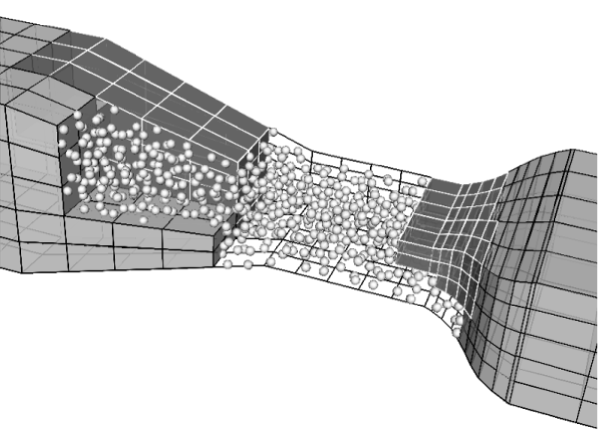
Figure 2: Example of a molecular dynamics flow simulation in a complex nano channel. The mesh is decomposed into five irregular portions, four of which are shown as shaded blocks, the molecules contained in the fifth portion are shown.

Neighbour lists are unsuitable when considering systems of arbitrary geometry, that may have been divided into irregular and complex mesh segments using standard mesh partitioning techniques (see, for example, figure 2) for two reasons:

1. Interprocessor molecule transfers: A molecule may cross an interprocessor boundary at any point in time (even part of the way through a timestep), at which point it should be deleted from the processor it was on and an equivalent molecule created on the processor on the other side of the boundary. Given that neighbour lists are constructed as lists of array indices, references or pointers to the molecule’s location in a data structure, deleting a molecule would invalidate this location and require searching to remove all mentions of it. Likewise, creating a molecule would require the appropriate new pair interactions to be identified. Clearly this is not practical. It is conventional to allow molecules to ‘stray’ outside of the domain controlled by a processor and carry out interprocessor transfers (deletions and creations) during the next neighbour list rebuild. This is only possible when the spatial region associated with a processor can be simply defined by a function relating a position in space to a particular cell on a particular processor (i.e. a uniform, structured mesh, representing a simple domain). In a geometry where the space in question is defined by a collection of individual cells of arbitrary shape, this is not possible. For example the location the molecule has ‘strayed’ to may be on the other side of a solid wall on the neighbour processor, or across another interprocessor boundary. For the molecule to end up unambiguously in the correct place, interprocessor transfers must happen as molecules cross a face.

2. Spatially resolved flow properties: MD simulations used for flow studies must be able to spatially resolve fluid mechanic and thermodynamic fields. This is achieved by accumulating and averaging measurements of the properties of molecules in individual cells of the same mesh that defines the geometry. If a molecule is allowed to stray outside of the domain controlled by a processor, as above, then it would not be unambiguous and automatic which cell’s measurement the molecule should contribute to.

While both of these problems could be mitigated by, for example, working out which cell a molecule outside the domain should be in on another processor and sending its information, doing so would result in an inelegant and inflexible arrangement with each additional simulation feature (i.e. a different measured variable or class of intermolecular potential) requiring special treatment.

We have, therefore, developed a new algorithm which is of comparable computational cost to neighbour lists, but designed to be powerful and generic for simulation in arbitrary geometries. As will be shown, neighbour lists also have some unfavourable features that could be improved upon.

2 Arbitrary Interacting Cells Algorithm (AICA)

2.1 Replicated Molecule Periodicity and Parallelisation

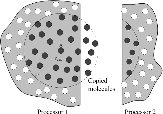
Figure 3: Domain decomposition. Molecule A must calculate intermolecular force contributions from all other molecules within its cut-off radius, $r_{cut}$. When the domain has been decomposed, some of these molecules may lie on a different processor. In this case, copies of the appropriate molecules from processor 2 are made on processor 1.

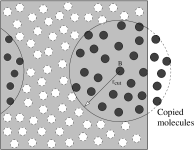
Figure 4: Periodic boundaries. Molecule B must calculate intermolecular force contributions from all other molecules within $r_{cut}$. Some of those molecules may be on a periodic image of the system, and as such, in implementation terms, will reside on the other side of the domain. Serial calculations in simple geometries typically use the minimum image convention [16, 19], but this is not suitable for parallelisation.

When parallelising an MD calculation, the spatial domain of the simulation is decomposed and each processor is given responsibility for a single region [16]. Molecules are, of course, able to cross the boundaries between these regions and therefore need to be communicated from one processor to the next. Processors also communicate when carrying out intermolecular force calculations, in which molecules close to processor boundaries need to be replicated on their neighbours to provide interactions. This process is illustrated in figure 3. Periodic boundaries also require information about molecules that are not adjacent physically in the domain (see figure 4), these required interactions can also be constructed by creating copies of molecules outside the boundary.

It is possible to handle processor and periodic boundaries in exactly the same way, since they have the same underlying objective: molecules near to the edge of a region need to be copied either between processors or to other locations on the same processor at every timestep to provide interactions. This is a useful feature because decomposing a mesh for parallelisation will often turn a periodic boundary into a processor boundary. The issue is how to efficiently identify which molecules need to be copied, and to which location, because this set continually changes as the molecules move.

2.2 Interacting Cell Identification

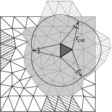
Figure 5: Interacting cell identification using unstructured triangular cells to demonstrate insensitivity to mesh topology. The spatial domain (main square section comprising the real cells) is periodic top-bottom and left-right. Real cells within $r_{cut}$ that interact with the CIQ (dark) are shaded in grey. The required referred cells are hatched in alternate directions according to which boundary they have been referred across. Realistic systems would be significantly larger compared to $r_{cut}$ than shown here.

The new Arbitrary Interacting Cells Algorithm (AICA) we propose here is an extension of the Conventional Cells Algorithm (CCA) [16]. In the CCA, a simple (usually cuboid) simulation domain is subdivided into equally sized cells. For computational and theoretical reasons, intermolecular potentials do not extend to infinity; they are assigned a cut-off radius, $r_{cut}$, beyond which they are set to zero. The minimum dimension of the CCA cells must be greater than $r_{cut}$, so that all molecules in a particular cell interact with all other molecules in their own cell and with those in their nearest neighbour cells (i.e. those they share a face, edge or vertex with — 26 in 3D). AICA uses the same type of mesh as would be used in Computational Fluid Dynamics (CFD) to define the geometry of a region. There are no restrictions on cell size, shape or connectivity. Each cell has a unique list of other cells that it is to interact with, this list is known as the Direct Interaction List (DIL) for the Cell In Question (CIQ). It is constructed by searching the mesh to create a set of cells that have at least one vertex within a distance of $r_{cut}$ from any of the vertices of the CIQ, see figure 5.

The DILs are established prior to the start of simulation and are valid throughout because the spatial relationship of the cells is fixed, whereas the set of molecules they contain is dynamic. In a similar way to the CCA, at every timestep a molecule in a particular cell calculates its interactions with the other molecules in that cell and consults the cell’s DIL to find which other cells contain molecules it should interact with. Information is required to be maintained stating which cell a molecule is in — this is straightforward and computationally cheap.

The construction of the DILs and accessing molecules is done in such a way as to not double-count interactions, similarly to the CCA. For example, if cells A and B need to interact, cell B will be on cell A’s DIL, but cell A will not be on cell B’s DIL. When a molecule in cell A interacts with one in cell B the molecule in cell B will receive the inverse of the force vector calculated to be added to the molecule in cell A, because the pair forces are reciprocal, i.e. $\mathbf{f_{ab}}=\mathbf{-f_{ba}}$.

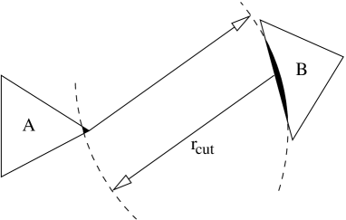
Figure 6: Errors caused by cut-off radius searching from vertices only. An arc of radius $r_{cut}$ drawn from the indicated vertex on cell A intersects a face of cell B, therefore, molecules near this vertex should interact with molecules in the shaded region. Similarly, an arc of radius $r_{cut}$ drawn from the indicated face on cell B encompasses the small shaded region of cell A. The cell searching algorithm will not, however, identify cells A and B as needing to interact because none of their vertices lie within $r_{cut}$ of each other.

It is possible in rare cases for small errors to be caused by this algorithm: small slices of volume in cells may not be identified for interaction (see figure 6). The errors introduced will be slight because the relative volume not accounted for will be very small: in figure 6, only when molecules are in both the indicated regions of each cell will either miss out on an interaction, and the intermolecular potential will be small at this distance. A small guard distance could be added to $r_{cut}$ when constructing the DIL to reduce this error. This is less of a problem in good quality meshes, e.g. hexahedral rather than tetrahedral cells.

2.2.1 Referred Molecules and Cells

Replicated molecule parallelisation and periodic boundaries are handled in the same way using referred cells (see figure 5) and referred molecules.

Referred molecule:

A copy of a real molecule that has been placed in a region outside a periodic or processor boundary in order to provide the correct intermolecular interaction with molecules inside the domain. A referred molecule holds only its own position and id (i.e. identification of which type of molecule it is for heterogenous simulations). Referred molecules are created and discarded at each timestep, and do not report any information back to their source molecules. Therefore if molecule j on processor 1 needs to interact with molecule k on processor 2, a separate referred molecule will be created on each processor.

Referred cell:

Referred cells define a region of space and hold a collection of referred molecules. Each referred cell knows

• which real cell in the mesh (on which processor) is its source;

• the required transformation to refer the positions and orientations of the real molecules in the source cell to the referred location (see below for the details of how cells and molecules are referred);

• the positions of all of its own vertices. These are the positions of the vertices of the source cell which have been transformed by the same referring transform as the referred molecules it contains;

• which real cells are in range of this particular referred cell and hence require intermolecular interactions to be calculated. This is constructed once at the start of the simulation in the same way as the DIL for real-real cell interactions — the vertices of the real cells in the portion of mesh on the same processor as the referred cell are searched, those with at least one vertex in range of any vertex of the referred cell are found.

2.2.2 Referring Transformations

A spatial transformation is required to refer a cell across a periodic or processor boundary. Figure 7 shows the most general case of a cell being referred across a separated, non-parallel boundary, where,

$\alpha^{0}$ =	Cell with a face on one side of the boundary.
$\beta^{0}$ =	Cell with a face on the other side of the boundary, coupled to $\alpha^{0}$
$\alpha^{1}$ =	Cell $\alpha^{0}$ referred across the boundary.
$\mathbf{C}$ =	Cell centre.
$\mathbf{n}$ =	Face normal unit vector.
$\mathbf{S_{\alpha^{0}\beta^{0}}}$ =	$\mathbf{C_{\beta^{0}}-C_{\alpha^{0}}}$. Position shift from $\mathbf{C_{\alpha^{0}}}$ to $\mathbf{C_{\beta^{0}}}$.
$\mathbf{R_{\alpha^{0}\beta^{0}}}$ =	Tensor required to rotate $\mathbf{-\hat{n}_{\alpha^{0}}}$ to $\mathbf{\hat{n}_{\beta^{0}}}$, given by,

$$\mathbf{R_{\alpha^{0}\beta^{0}}=-\left(n_{\alpha}\cdot n_{\beta}\right)I}+\left(1+\mathbf{n_{\alpha}\cdot n_{\beta}}\right)\mathbf{\left(\frac{n_{\alpha}\times n_{\beta}}{\left|n_{\alpha}\times n_{\beta}\right|}\right)^{2}+n_{\alpha}n_{\beta}-n_{\beta}n_{\alpha}},$$ (1)

where $\mathbf{I}$ is the identity tensor. The absolute position, $\mathbf{P^{\prime}}$, of a molecule has been transformed across a boundary (with its containing cell) from its original position, $\mathbf{P}$ is required. To derive the $\mathbf{P\rightarrow P^{\prime}}$ transform, first the position of $\mathbf{P}$ relative to centre of the coupled face on $\alpha^{0}$ is given as,

$$\mathbf{P-C_{\alpha^{0}}}.$$ (2)

Then this vector is rotated by the transformation tensor defined by the source and destination coupled face normals,

$$\mathbf{R_{\alpha^{0}\beta^{0}}\cdot\left(P-C_{\alpha^{0}}\right)}.$$ (3)

The rotated position is transformed back to global coordinates,

$$\mathbf{C_{\alpha^{0}}+R_{\alpha^{0}\beta^{0}}\cdot\left(P-C_{\alpha^{0}}\right)},$$ (4)

and then shifted by the relative separation of the coupled face centres, i.e.

$$\mathbf{P^{\prime}} =\mathbf{C_{\alpha^{0}}+S_{\alpha^{0}\beta^{0}}+R_{\alpha^{0}\beta^{0}}\cdot\left(P-C_{\alpha^{0}}\right)},$$

$$=\mathbf{C_{\alpha^{0}}+C_{\beta^{0}}-C_{\alpha^{0}}+R_{\alpha^{0}\beta^{0}}\cdot\left(P-C_{\alpha^{0}}\right)},$$

$$=\mathbf{C_{\beta^{0}}-R_{\alpha^{0}\beta^{0}}\cdot C_{\alpha^{0}}+R_{\alpha^{0}\beta^{0}}\cdot P}.$$ (5)

The result is the same if the point is shifted by $\mathbf{S_{\alpha^{0}\beta^{0}}}$ prior to rotation by $\mathbf{R_{\alpha^{0}\beta^{0}}}$ around $\mathbf{C_{\beta^{0}}}$. The final position of $\mathbf{P^{\prime}}$ is the same if any coupled face centre/face normal pair on the boundary is used. Therefore, all cells and all molecules referred across a particular boundary may use the transformation derived from one cell.

This result can be used to transform the positions of all of the molecules in a source cell to their correct position in a referred cell. Molecules being referred also operate on their own rotationally dependant properties (e.g. angular orientation) using the rotation tensor. This transformation is suitable for multiple periodic boundaries and arbitrary mesh decompositions where existing referred cells must be re-referred by other boundaries. This creates the cell relationships across edges, corners, and also on non-neighbouring processors. See Appendix B for an example. Cell re-referring is achieved by writing equation (5) as a generic transform,

$$\mathbf{P^{\prime}=y+R\cdot P},$$ (6)

where,

$$\mathbf{y} =\mathbf{C_{\beta^{0}}-R_{\alpha^{0}\beta^{0}}\cdot C_{\alpha^{0}}},$$ (7)

$$\mathbf{R} =\mathbf{R_{\alpha^{0}\beta^{0}}}.$$ (8)

If $\mathbf{y}$ and $\mathbf{R}$ are the transformations required to move $\mathbf{P}$ to $\mathbf{P^{\prime}}$, then transforming $\mathbf{P^{\prime}}$ to $\mathbf{P^{\prime\prime}}$ using $\mathbf{y^{\prime}}$ and $\mathbf{R^{\prime}}$ gives,

$$\mathbf{P^{\prime\prime}} =\mathbf{y^{\prime}+R^{\prime}\cdot P^{\prime}},$$

$$=\mathbf{y^{\prime}+R^{\prime}\cdot y+R^{\prime}\cdot R\cdot P},$$

$$=\mathbf{y^{\prime\star}+R^{\prime\star}\cdot P},$$ (9)

reduced to the generic form by defining,

$$\mathbf{y^{\prime\star}} =\mathbf{y^{\prime}+R^{\prime}\cdot y},$$ (10)

$$\mathbf{R^{\prime\star}} =\mathbf{R^{\prime}\cdot R}.$$ (11)

Further re-referrals can be reduced to a single transform in a predictable way, with only a single vector/tensor pair required to be stored by the referred cell at any stage. Any number of cell referring transformations may be made sequentially, but the resulting transformation takes the initial source position ($\mathbf{P}$) and directly transforms it to the final destination, regardless of, and without having to intermediately visit, the other referred locations along the way.

2.3 Intermolecular Force Calculation Algorithm Details

At the start of the simulation, the DIL for each cell are created, referred cells are created and they determine which real cells they must supply interactions to. Details of how these are constructed can be found in Appendix A. Cells requiring to be referred need not be on processors sharing a boundary with their destination processor, i.e. AICA must be able to identify interactions between non-neighbouring processors. However, when constructing the referred cells, processors may only communicate across interprocessor faces, i.e. with neighbours only.

The geometry of the system is defined by a 3D, static, unstructured mesh. A cell’s position in the data structure, hence its index, does not imply anything about its physical location or connectivity. Therefore, the ability to handle arbitrary geometries comes from deducing locally which cells are in range to interact. The same net force on any molecule will be calculated irrespective of cell size and shape (except in rare instances, see section 2.2).

The total intermolecular force acting upon a molecule is calculated at each timestep by considering two types of interactions. Real-Real interactions occur between a molecule and others on the same processor. Real-Referred interactions occur between real molecules and referred molecules arising from the other side of a processor or periodic boundary. Referred molecules do not need to calculate interactions between themselves, because every referred molecule is a copy of a real molecule elsewhere, and as such will receive all of its real-real and real-referred interactions in-situ.

2.3.1 Real-Real Molecule Force Calculation

At each time step, the real molecules on each processor calculate their intermolecular interactions as follows:

for all cells, denoted I {
    for all molecules in cell I, denote mol k
    {
        for all cells in cell I’s DIL, denote cell J
        {
            for all molecules in cell J, denote mol l
            {
                calculate intermolecular force, Fkl,
                between mol k and mol l.
                Add Fkl to mol k, add Flk = -Fkl to mol l.
            }
        }

        for all molecules in cell I, denote mol k’
        {
            if index of, or pointer to, mol k’ > mol k
            then calculate intermolecular force, Fkk’,
            between mol k and mol k’.
            Add Fkk’ to mol k, add -Fkk’ to mol k’.
        }
    }
}

Comparison of the index, or pointer to molecules in the same cell, mol k’ > mol k, means that interactions between molecules in the same cell are not double counted and a molecule does not calculate an interaction with itself. The order of comparison is not important, as long as all pairs are covered, so using mol k’ < mol k as a condition would work equally well.

2.3.2 Real-Referred Molecule Force Calculation

At each timestep all real cells which are the source cell of one or more referred cells send the position and id of all of the molecules they contain to the appropriate referred cell on the appropriate processor. The destination referred cells perform the appropriate position and orientation transformation when the molecules are received. These referred molecules calculate their intermolecular interactions with real molecules as follows:

for all referred cells, denoted M {
    for all referred molecules in referred cell M, denote mol q
    {
        for all real cells that referred cell M
        interacts with, denote cell N
        {
            for all real molecules in cell N, denote mol p
            {
                calculate intermolecular force, Fpq,
                between mol p and mol q.
                Add Fpq to mol p.
            }
        }
    }
}

2.4 Prediction of Computational Speed

The following analysis determines whether or not AICA is practical, by predicting its computational cost relative to that of the CCA and Neighbour List Algorithm (NLA).

Assuming a system of approximately uniform density, the volume of space around a particular molecule to be interrogated by a particular algorithm will be directly proportional to the number of pair interactions to be evaluated, which is itself directly proportional the computational cost per timestep. For a given cut off radius, $r_{cut}$, the volume associated with a particular algorithm is:

Ideal:

Evaluating the minimum possible number of pairs is equivalent to a sphere of radius $r_{cut}$,

$$V_{ideal}=\frac{4}{3}\pi r_{cut}^{3}.$$ (12)

However, it is not possible to design an algorithm that only evaluates the ideal case because the relative spatial arrangement of molecules is not known in advance from one timestep to the next.

CCA:

The volume encompassed by the CCA depends on the cell size — it is minimum when cells are cubic with side length $r_{cut}$. The volume of the cell containing the molecule in question, plus that of its 26 neighbours is encompassed, giving

$$V_{CCA}=27r_{cut}^{3}.$$ (13)

NLA:

The neighbour list for a particular molecule includes all molecule interaction pairs within a sphere of radius $r_{cut}$ plus a guard distance $\Delta R$ [16]. It is constructed using the CCA, where the cells must be at least $r_{cut}+\Delta R$ in size, and has a lifetime of $L$ timesteps before invalidation. Therefore, each timestep that the neighbour list is used for must absorb a fraction of the CCA cost required to construct the list — the shorter the lifetime of the neighbour list, the more costly the NLA becomes. Therefore,

$$V_{NLA}=\frac{4}{3}\pi\left(r_{cut}+\Delta R\right)^{3}+\frac{27}{L}\left(r_{cut}+\Delta R\right)^{3}.$$ (14)

AICA:

The volume encompassed by AICA is the total volume of all cells which have at least one vertex within $r_{cut}$ of any vertex of the cell containing the molecule in question, plus the volume of this cell. This depends on the local topology of the mesh. As a simple example, consider a uniform mesh of cubes of side length $w$. A piecewise function, $N_{c}(r_{cut}/w)$ has been derived to count the number of cubes, each of volume $w^{3}$, that have at least one corner within a distance of $r_{cut}/w$ of a corner of a central cube (which is included). In this case,

$$V_{AICA}=N_{c}(r_{cut}/w)w^{3}.$$ (15)

These volumes are plotted on figure 8 with $w/r_{cut}$ as the independent variable, lower values of $w/r_{cut}$ representing a finer mesh for a given cut-off radius. AICA is costlier than the CCA or NLA in coarse meshes, however, when $w\lesssim 0.4r_{cut}$ (see inset for detail) AICA has a similar computational cost to the NLA, for the chosen representative values of $L$ and $\Delta R$. The discontinuities in $V_{AICA}$ are due to the steps in $N_{c}(r_{cut}/w)$ which arise when a threshold is crossed and another ‘layer’ of cubes is required.

While real meshes in complex geometries will not comprise uniform cubes, this result demonstrates that AICA can be of comparable speed to the NLA, and gives an indication of the required refinement. As the mesh becomes finer, the set of cells selected to interact with the cell at the centre becomes an increasingly accurate approximation of the ideal sphere, this can be seen in the $V_{AICA}$ function, which asymptotically approaches $V_{ideal}$ as $w/r_{cut}\rightarrow 0$. Note that, in this example, AICA and the CCA are equivalent when $w/c_{cut}=1$ because their cells are the same size.

2.4.1 Neighbour List Lifetime Prediction

The computational cost of the neighbour list algorithm depends on the number of timesteps a neighbour list remains valid for — a quantity whose dependence on simulation properties can be predicted.

For a given number of molecules, $N$, of mass $m$, in equilibrium at a temperature $T$, there is a probability of $1/N$ that a molecule in the system will be travelling with a velocity $v_{N}$. It is therefore likely that at every timestep there will be one molecule travelling at, or close to this velocity. Given that a neighbour list is invalidated when the cumulative sum of maximum displacements in the system exceeds a fixed threshold (usually $0.5\Delta R$, half the guard radius [16]), finding the number of timesteps required for a molecule travelling at $v_{N}$ to cover this distance gives an estimate of the lifetime of the list.

Finding $v_{N}$ by equating the Maxwellian velocity distribution to $1/N$, where $T$, $m$ and $v_{N}$ are in reduced MD units [19] (see figure 9):

$$4\pi\left(\frac{m}{2\pi T}\right)^{\frac{3}{2}}v_{N}^{2}e^{\left(\frac{-mv_{N}^{2}}{2T}\right)}=\frac{1}{N}.$$ (16)

The high speed solution is,

$$v_{N}=\sqrt{-\frac{2T}{m}W_{-1}\left(-\frac{1}{4N}\sqrt{\frac{2\pi T}{m}}\right)},$$ (17)

where $W_{-1}$ is the secondary real branch of the Lambert W function. Therefore, $L$, the number of timesteps (of length $\Delta t$) a neighbour list is valid for, is given by

$$L=\left\lceil\frac{0.5\Delta R}{\Delta tv_{N}}\right\rceil.$$ (18)

This lifetime reduces with increasing temperature and system size, as shown in figure 10, resulting in a higher computational cost for the NLA. At higher temperatures, $v_{N}$ is higher because the velocity distribution covers a higher molecular speed range. In systems comprising more molecules, it is more probable that at least one molecule will be travelling at a given speed in the upper region of the distribution, therefore $v_{N}$ is also higher.

The cost of AICA is not sensitive to either of these parameters, therefore it becomes increasingly attractive in large systems ($>10^{6}$ molecules) where neighbour list lifetimes are low.

3 Implementation and Verification

AICA has been implemented in OpenFOAM [20, 21], which is an open source C++ library intended for continuum mechanics simulation of user-defined physics (primarily used for CFD) in arbitrary, unstructured geometries. The AICA MD code has been built using OpenFOAM’s lagrangian particle tracking library, which has been used to track particles in solution, droplets in combusting diesel sprays and to perform DSMC simulations [22].

The AICA algorithm must show that it produces the correct results, assessed by momentum and energy conservation and the behaviour of average potential and kinetic energy, in three ways:

1. The code must produce the same results as another (validated) MD code. For these purposes the other code is an in-house MD code which has been validated against those supplied in[16].

2. The results for the AICA MD code must be the same whether it is run on one processor as a serial calculation, or run in parallel on many distributed CPUs.

3. The topology of the underlying mesh must not make any difference to the results.

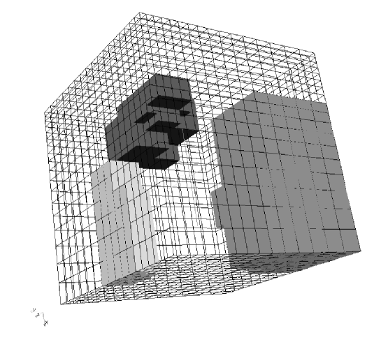
Figure 11: Mesh for the serial vs. parallel test; note the grading of cells. The serial test uses the whole mesh (wireframe) and the parallel test decomposes the mesh into 24 portions (3 of which have been shown).

The serial/parallel test case for AICA is shown in figure 11. The test mesh is decomposed into 24 portions, the three examples shown are not regular shapes and the cells are nonuniform in size (the mesh is graded in each direction). While this test mesh is structured, the algorithm makes no use of this fact, so a mesh comprising cells of any size, shape or connectivity would produce the same result. This case will therefore demonstrate the independence of the AICA from the form of the geometry used.

Figures 12, 13 and 14 show the average kinetic (KE), potential (PE) and total (TE) energy per molecule for a system containing 27000 Lennard Jones molecules, starting in a simple cubic lattice at a temperature of 120K. No equilibration or thermostat has been applied. Results for the in-house code, the AICA code in serial on a PC and the AICA code decomposed and run on 24 processors of a cluster show that the KE and PE graphs follow very similar trends to the in-house code. The simulations do not follow exactly the same trajectory because the velocities in the systems are initialised by random numbers, which are different between the two codes. This is likely to account for the slight (0.0025%) difference in average TE. The serial and parallel tests use the same initial velocity configuration and each value for KE, PE and TE are the same to better than 1 part in $10^{12}$. Momentum is conserved in both serial and parallel tests to approximately 1 part in $10^{16}$.

Given that the serial and parallel results are exactly the same, the AICA must be creating the correct referred cells and molecules, and calculating real-referred interactions perfectly, even with the relatively complex decomposed portions of the mesh.

A comparison of how the computational speed changes with mesh refinement, compared to the predictions in section 2.4, and further tests of how the AICA performance scales in parallel will appear in a future publication.

4 Conclusions

Our Arbitrary Interacting Cell Algorithm (AICA) has been described, which is a new way of calculating pair forces in a molecular dynamics simulation, carried out on an arbitrary unstructured mesh that has been spatially decomposed to run in parallel. The algorithm is expected to achieve a similar computational speed to the neighbour list method, but does not suffer from the identified degradations in performance that neighbour lists experience in large systems and at high temperatures. AICA has been implemented in the OpenFOAM code, and produces the same results when a system is simulated in serial, or in parallel on a mesh decomposed into irregular shapes on 24 processors. The exchange of intermolecular force information across interprocessor boundaries must therefore be correct.

Currently this algorithm deals only with short ranged pair forces. Future developments will include rigid and flexible polyatomic molecules, and long-range electrostatic forces. A hybrid MD/continuum implementation in OpenFOAM is currently under development. OpenFOAM is ideal for incorporating polar fluids and electrokinetic actuation, which feature in envisioned applications, because it is able to simulate electromagnetic, magnetohydrodynamic and fluid mechanic continuum fields on the same mesh that AICA operates with.

5 Acknowledgements

The authors would like to thank Chris Greenshields and Matthew Borg of Strathclyde University (UK), and Henry Weller and Mattijs Janssens of OpenCFD Ltd. (UK) for useful discussions. This work is funded in the UK by Strathclyde University and the Miller Foundation, and through a Philip Leverhulme Prize for JMR from the Leverhulme Trust.

Appendix A Cell Interactions

Building interaction lists and identifying and creating referred cells is allowed to be computationally expensive (within reason) because it will only happen once at the beginning of the MD simulation. Accessing the information, however, must be as fast as possible because it will happen at every timestep.

Cell interactions are based on the largest cut-off radius of any intermolecular potential in a heterogenous system, $\hat{r}_{cut}$. It is possible to have different interaction lists when potentials with substantially different cut-off radii are used.

A.1 Building DILs

To create each real cell’s DIL, a non double counting loop through all cells is used, where the cells are accessed by an index ($i$ or $j$) running $0\rightarrow k-1$, where there are $k$ cells in the portion of mesh on the processor in question, i.e.

for cells, denote cell i, starting i = 0, while i < k-1 {
    for cells, denote cell j, starting j = i+1, while j < k
    {
        calculate magnitude of spatial separation of all
        vertices of cell i with all vertices of cell j.

        if any separation distance is less than the
        maximum cut off radius, add cell j to cell i’s DIL.
    }
}

For example, if there are $k=5$ cells, the array index runs from $0\rightarrow 4$:

$i$	$j$
$0$	$1,2,3,4$
$1$	$2,3,4$
$2$	$3,4$
$3$	$4$

All cell combinations have been created once, i.e. when $i=2$, $j=1$ would produce the 2–1 combination, which is already identified as 1–2. This non double counting procedure means that some cells will have few or no other cells in their DIL, however, as long as the correct cell pair is created in one of the cell’s DIL, this is not an issue. It is also designed so that a cell does not end up on its own DIL, the interactions between molecules in the same cell are handled separately.

A.2 Creating Referred Cells

Coupled patches are the basis of periodic and interprocessor communication for creating referred cells. Patches, in general, are a collection of cell faces representing a mesh boundary of some description — they may provide solid surfaces, inlets, outlets, symmetry planes, periodic planes, or interprocessor connections. Coupled patches provide two surfaces; whatever exits one enters the other and vice versa. Two types are used in AICA:

• Periodic patches on a single processor are arranged into two halves, each half representing one of the coupled periodic surfaces. When a molecule crosses a face on one surface, it is wrapped around to the corresponding position on the corresponding face on the other surface.

• Processor patches provide links between portions of the mesh on different processors, one half of the patch is on each processor. When a molecule crosses a face on one surface, it is moved to the corresponding position on the corresponding face on the other surface, on the other processor. Decomposing a mesh for parallelisation will often require a periodic patch to be changed to a processor patch.

The surfaces of coupled patches may have any relative orientation, and may be spatially separated as long as the face pairs on each surface correspond to each other. This allows them to also be used as a ‘recycling’ surface in a flow simulation — whatever exits from an outlet is reintroduced at an inlet, with the option of scaling the molecule’s properties, e.g. temperature and pressure.

A.2.1 Create Patch Segments.

In the decomposed portion of the mesh on each processor, each processor and periodic patch should be split into segments, such that:

• faces on a processor that were internal to the mesh prior to decomposition end up on a segment;

• faces on a processor patch that were on separate periodic patches on the undecomposed mesh end up on different segments. These segments are further split such that faces that were on different halves of the periodic patch on the undecomposed mesh end up on different segments;

• faces on different halves of a periodic patch end up on different segments.

Each segment must produce a single vector/tensor transformation pair (see section 2.2.2) which will be applied to all cells referred across it.

A.2.2 Cell Referring Iterations.

For each patch segment:

1. Find all real and existing referred cells in range (with at least one vertex within a distance of $\hat{r}_{cut}$) of at least one vertex of the faces comprising the patch segment.

2. Refer or re-refer this set of cells across the boundary defined by the patch segment using its transformation, see section 2.2.2. In the case of a segment of periodic boundary, this creates new referred cells on the same processor. For a segment of a processor patch, these cells are communicated to, and created on the neighbouring processor. Before creating any new referred cell a check is carried out to ensure that it is not

   • a duplicate referred cell, one that has been created already by being referred across a different segment;

   • a referred cell trying to be duplicated on top of a real cell, i.e. a cell being referred back on top of itself.

   If the proposed cell for referral would create a duplicate of an existing referred cell, or end up on top of a real cell, then it is not created. To be a duplicate, the source processor, source cell and the vector part of the transformation (see section 2.2.2) must be the same for the two cells (note, the vector part of transformation for a real cell is zero by definition).

A single run of these steps will usually not produce all of the required referred cells. They are repeated until no processor adds a referred cell in a complete evaluation of all segments, meaning all possible interactions are accounted for. In iterations after the first, in step 1 it is enough to only search for referred cells in range of the faces on the patch segment, because the real cells will not have changed, and would all be duplicates. The final configuration of referred cells does not depend on the order of patch segment evaluation. Appendix B contains an example of the results of the cell referring process.

Appendix B Example Construction of Referred Cells

Figures 15 and 16 show the start and end points of the cell referring operation on a mesh that has been decomposed to run in parallel. The example is in 2D for clarity but the process is exactly the same in 3D.

In this example the number of referred cells created far exceeds the number of real cells, which would lead to much costly interprocessor communication. This is because the mesh has been made deliberately small relative to $\hat{r}_{cut}$ to demonstrate as many features of the algorithm as possible and to be practical to understand. In realistic systems, the mesh portions would be significantly bigger than $\hat{r}_{cut}$ and the referred cells would form a relatively thin ‘skin’ around each portion. Decomposition of the mesh should preferably be carried out to minimise the number of cells that need to be referred, and to ensure that the vast majority of the intermolecular interactions happen between real-real molecule pairs; in this way the communication cost is minimised.

Figure 7: A molecule at point $\mathbf{P}$ is referred across the boundary (heavy line) to $\mathbf{P^{\prime}}$ by a transformation defined by the face center/face normal vectors of the faces of cells $\alpha^{0}$ and $\beta^{0}$ on the boundary. The mesh is rigid, so all points of cell $\alpha^{1}$ have the same relative spatial relationship as $\alpha^{0}$. The vertices of referred cell $\alpha^{1}$ are calculated by the same process.

Figure 8: Predicted computational cost of new AICA using cubic cells, compared with conventional algorithms. $\Delta R=0.16r_{cut}$ derived from typical values for liquid density simulation $r_{cut}=2.5$, $\Delta R=0.4$ [16].

Figure 9: Maxwellian velocity distribution. Finding velocities corresponding to a probability of $1/N$, where $N$ is the number of molecules in the system. There are two real, positive solutions — the high speed one is $v_{N}$, the quantity of interest.

Figure 10: Variation of estimated neighbour list lifetime with typical simulation parameters for a Lennard Jones fluid [16]. $T,m,\Delta R$ and $\Delta t$ are in reduced MD units.

Figure 12: Verification of kinetic energy results. Serial and parallel results are identical, see inset.

Figure 13: Verification of potential energy results. Serial and parallel results are identical, see inset.

Figure 14: Verification of total energy results. Serial and parallel results are identical, see inset.

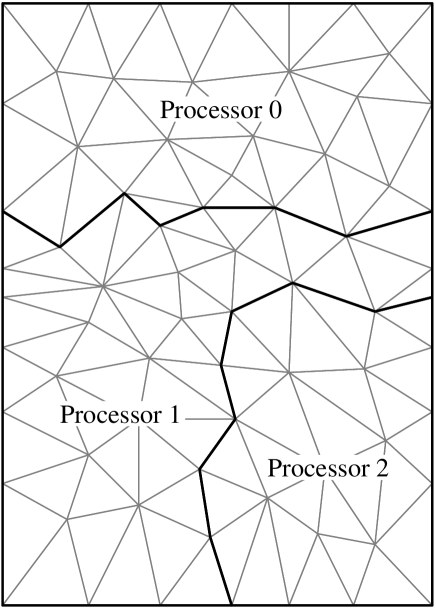
Figure 15: An arbitrary unstructured mesh, which is periodic top-bottom and left-right. It is decomposed into 3 irregular portions for parallel processing as marked.

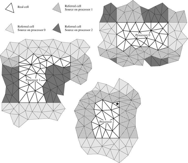
Figure 16: The final configuration of referred cells around the portions of the mesh in figure 15 on each processor. A circle of radius $\hat{r}_{cut}$ drawn from any vertex of a real cell would be fully encompassed by other real or referred cells, thereby providing all molecules in that cell with the appropriate intermolecular interactions, either across a periodic boundary or from another processor. Note that many cells are referred several times; for example, the source cell marked with $\bigstar$ on processor 2 is referred to processors 0 and 1 twice on each.

References

- [1] P. Agre, The aquaporin water channels, Proceedings of the American Thoracic Society 3 (1) (2006) 5–13.
- [2] J. Koplik, J. R. Banavar, Continuum deductions from molecular hydrodynamics, Annual Review of Fluid Mechanics 27 (1995) 257–292.
- [3] H. Brenner, V. Ganesan, Molecular wall effects: are conditions at a boundary “boundary conditions”?, Physical Review E 61 (6) (2000) 6879–6897.
- [4] D. Hirshfeld, D. Rapaport, Molecular dynamics simulation of Taylor-Couette vortex formation, Physical Review Letters 80 (24) (1998) 5337–5340.
- [5] D. Rapaport, E. Clementi, Eddy formation in obstructed fluid flow: a molecular-dynamics study, Physical Review Letters 57 (6) (1986) 695–698.
- [6] K. Travis, B. Todd, D. Evans, Poiseuille flow of molecular fluids, Physica A 240 (1-2) (1997) 315–27.
- [7] K. Travis, B. Todd, D. Evans, Departure from Navier-Stokes hydrodynamics in confined liquids, Physical Review E 55 (4) (1997) 4288–95.
- [8] T. Qian, X.-P. Wang, Driven cavity flow: from molecular dynamics to continuum hydrodynamics, Multiscale Modeling and Simulation 3 (4) (2005) 749–763.
- [9] T. Becker, F. Mugele, Nanofluidics: viscous dissipation in layered liquid films, Physical Review Letters 91 (2003) 166104.
- [10] H. Okumura, D. M. Heyes, Comparisons between molecular dynamics and hydrodynamics treatment of nonstationary thermal processes in a liquid, Physical Review E 70 (6) (2004) 061206.
- [11] R. Delgado-Buscalioni, P. V. Coveney, Hybrid molecular-continuum fluid dynamics, Philosophical Transactions of the Royal Society London 362 (1821) (2004) 1639–1654.
- [12] G. Wagner, E. G. Flekkøy, Hybrid computations with flux exchange, Philosophical Transactions of the Royal Society London 362 (1821) (2004) 1655–1665.
- [13] X. B. Nie, S. Y. Chen, W. E, M. O. Robbins, A continuum and molecular dynamics hybrid method for micro- and nano-fluid flow, Journal of Fluid Mechanics 500 (2004) 55–64.
- [14] T. Werder, J. H. Walther, P. Koumoutsakos, Hybrid atomistic-continuum method for the simulation of dense fluid flows, Journal of Computational Physics 205 (1) (2005) 373–390.
- [15] S. Pennathur, J. G. Santiago, Electrokinetic transport in nanochannels. 2. experiments, Analytical Chemistry 77 (21) (2005) 6782–6789.
- [16] D. C. Rapaport, The Art of Molecular Dynamics Simulation, 2nd ed., Cambridge University Press, 2004.
- [17] W. Smith, Molecular dynamics on hypercube parallel computers, Computer Physics Communications 62 (2–3) (1991) 229—248.
- [18] D. Rapaport, Multi-million particle molecular dynamics. II. Design considerations for distributed processing, Computer Physics Communications 62 (2–3) (1991) 217–228.
- [19] M. Allen, D. Tildesley, Computer simulation of liquids, Oxford University Press, 1987.
- [20] H. G. Weller, G. Tabora, H. Jasak, C. Fureby, A tensorial approach to computational continuum mechanics using object-oriented techniques, Computers in Physics 12 (1998) 620–631.
- [21] OpenFOAM, www.openfoam.org.
- [22] J. Allen, T. Hauser, foamDSMC: An object oriented parallel DSMC solver for rarefied flow applications, in: 45th AIAA Aerospace Sciences Meeting and Exhibit, Reno, Nevada, 2007.