Certifying controls and systems software

Abstract

Software system certification presents itself with many challenges, including the necessity to certify the system at the level of functional requirements, code and binary levels, the need to chase down run-time errors, and the need for proving timing properties of the eventual, compiled system. This paper illustrates possible approaches for certifying code that arises from control systems requirements as far as stability properties are concerned. The relative simplicity of the certification process should encourage the development of systematic procedures for certifying control system codes for more complex environments.

1 Introduction

Discussions about analyzing software in a controls framework often oscillate between trivial statements and feelings of doom dominated by undecidability issues. Furthermore much of the intrinsic difficulty (or lack thereof) of software analysis, even that designed by control systems engineers, hides behind an intimidating language barrier, making tools and concepts developed by computer scientists hard to reach by controls specialists, and vice-versa. This paper concentrates on the following question: Given a properly designed system (presumably a stable control system), what else needs to be proven to convince the certification agency that the behavior is indeed appropriate? We argue that the concept of “proof of good behavior” as currently taught in the control systems curriculum mostly focuses at the level of “system specification”, meaning at a level where the system is unambiguously defined, but does not constitute an executable code yet. By means of example, consider the system

$$x_{k+1}=Ax_{k},\;\;k=0,1,\ldots\;\;\;x_{0}\in\mathrm{\mathbf{R}}^{n},\;\;x_{0}^{T}x_{0}\leq 1$$ (1)

and ask whether the state $x$ is always bounded. This question is usually answered by checking various sufficient conditions such as (i) all eigenvalues of $A$ have modulus strictly less than one, or (ii) there exists a symmetric, positive definite matrix P satisfying the Lyapunov inequality

$$A^{T}PA-P<0.$$

While much of the control systems community would consider the job to be “done”, the fact is that the system (1) is not considered “executable” except for high-level, non real-time environments such as MATLAB. The program described in flowchart format in Fig. 1 is the accurate representation of what a real-time, computer implementation of the system (1) might be. Discussing the system (1) at the level of the flowchart shown in Fig. 1 might be dismissed by many as an “implementation issue”. This opinion must, however, face the following facts: (i) Certification agencies tend to look at all levels of system implementation and not only the specification level (1); (ii) the development of code is often not performed by the same agent that developed the program specifications, thus introducing doubt as to whether the specification has been faithfully implemented; and (iii) providing the certification agency with code-level assurance of proper behavior does not require much effort, which is our main point today: The next section of our paper discusses simple, generic philosophies when establishing “program proofs”, and argues in favor of an “instruction-by-instruction” analysis approach. This discussion is then applied to describe what constitutes a “proof” for the program shown in Fig. 1.

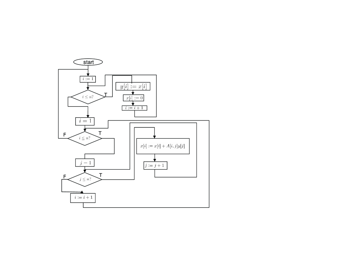
Figure 1: Program in flow-chart form

We then conclude this article by suggesting easy extensions of our discussion.

2 Proving computer programs: Gathering meaning first or not?

When analyzing code, a central issue is the design of what is called the collecting semantics. The collecting semantics describes how much information from the original program must be retained and compiled in order to verify the desired property (eg variable boundedness). The collecting semantics forms the base model on which the analysis is conducted. Higher levels of semantic collection allow one to define more compact models of the software execution, but this task may also be more complex, since information must be collected over several lines of code and then linked into a compact model. Thus, lower semantic levels (like line-by-line analyses) are more desirable from the standpoint of analyzer simplicity and adaptability. They may also improve analysis readability, by linking the analysis closely to the code itself and remembering that the value of any code analysis improves if it is more readable. The process that favors high-level semantics collection first, followed by the analysis of such semantics would correspond to taking the code in Fig. 1,proving it matches the system specification (1), and proving the specification (1) is indeed stable using eigenvalue or other stability. Such an approach was implemented, for example, in Cousot’s ASTRÉE analyzer [Fer04, BCC⁺03b, BCC⁺03a], which was used to support the certification process for several large commercial aircraft.

In contrast, the process that favors lower semantics levels, such as “line-by- line’ analyses would take the code in Fig. 1 and the system specification (1) to build a proof that the code satisfies the desired stability property.

The net result is a much more detailed analysis of the code at a level that stands much closer to its eventual implementation. Another key observation is to realize that once written, this proof does not require the system specification 1 to be understood and independently verified. A key tool for line-by-line analysis may be found in [Pel01, Ch.7], where the author describes a technique for line-by-line analysis by means of invariants: In this analysis, which dates back to the 1960’s, each line of code corresponds to either a test or an assignment. A test has one entry channel and two exit channels (one for the case when the test is true, and one for when the test is false). An assignment has one input channel and one output channel, and consists of a variable update by means of a domainspecific operation. In the code described in Fig. 1, tests are shown in diamond-shaped boxes, while assignments are shown in rectangular boxes. For each line of code, two invariant properties of the code state are guessed: The pre-instruction invariant describes a set to which the code state always belongs prior to instruction execution. The post-instruction invariant(s) describe set(s) to which the variables always belong after the execution of the instruction. Given two consecutive instructions named 1 and 2, if the post-instruction invariant of 1 is the same as the pre-instruction invariant of 2, then the two instructions can be composed with the guarantee that the pre-instruction of instruction 1 implies the post-instruction invariant of instruction 2. If such compatibility conditions hold over the whole program, then it is possible to use such mechanisms to prove that an entire program is “correct”. The appeal of such a method is that the elements of proof are distributed throughout the code, and may be independently verified instruction by instruction either manually or using the help of a computer, with no need to understand the whole “meaning’ of the program. 2 Proving the implementation of a linear system Consider now the code described in Fig. 1. We use our previous discussion to show that the correctness of such a code may be established on a line-by-line basis using ellipsoidal invariants. In the context of this section, we will say the program is correct if, for bounded initial conditions, the variables inside the program are all bounded. This observation becomes trivial once we recognize that (i) the proper state-space for the code consists of $x$, $y$ and the index variables $i$ and $j$ and (ii) all operations involving the computer variables $x$ and $y$ are linear in $x$ and $y$. From a theoretical perspective, describing the code behavior by means of ellipsoidal invariants adds little more to the story than simply describing it by means of (quadratic) Lyapunov functions. However, we find that ellipsoids are easier to manipulate, in that they eliminate inconvenient singular matrix inverse computations.

3 Behavior of state variables

The solution to the problem begins with realizing that the relevant state-space includes both $x$ and $y$, and that the transformations on $x$ and $y$ are linear in $x$ and $y$. For example, the instruction

$$y[i]:=x[i]$$

is a linear transformation that may also be written

$$\left[\begin{array}[c]{c}y\\ x\end{array}\right]=\left[\begin{array}[c]{cc}I-e_{ii}&e_{ii}\\ 0&I\end{array}\right]\left[\begin{array}[c]{c}y\\ x\end{array}\right]=S_{i}\left[\begin{array}[c]{c}y\\ x\end{array}\right]$$ (2)

where $e_{ij}$ is a matrix made of zeros everywhere, except at the entry on the $i$th row and $j$th column which is 1. Likewise, the instruction

$$x[i]:=0$$

is the linear transformation

$$\left[\begin{array}[c]{c}y\\ x\end{array}\right]=\left[\begin{array}[c]{cc}I&0\\ 0&I-e_{ii}\end{array}\right]\left[\begin{array}[c]{c}y\\ x\end{array}\right]=P_{i}\left[\begin{array}[c]{c}y\\ x\end{array}\right]$$ (3)

and the instruction

$$x[i]:=x[i]+A[i,j]y[j]$$

is the linear transformation

$$\left[\begin{array}[c]{c}y\\ x\end{array}\right]=\left[\begin{array}[c]{cc}I&0\\ A[i,j]e_{ij}&I\end{array}\right]\left[\begin{array}[c]{c}y\\ x\end{array}\right]=T_{ij}\left[\begin{array}[c]{c}y\\ x\end{array}\right]$$ (4)

After a full cycle, the net effect is for $x$ and $y$ to have gone through the multiplexed operation:

$$\left[\begin{array}[c]{c}y\\ x\end{array}\right]=\left[\begin{array}[c]{cc}0&I\\ 0&A\end{array}\right]\left[\begin{array}[c]{c}y\\ x\end{array}\right]=A_{1}\left[\begin{array}[c]{c}y\\ x\end{array}\right]$$ (5)

4 Ellipsoids

We use ellipsoidal invariants before and after each instruction in the program. Ellipsoids (centered around the origin) are usually defined as

$$\left\{z\in\mathrm{\mathbf{R}}^{n}\;\left|\;z^{T}Pz\leq 1\right.\right\},$$ (6)

where $P$ is a symmetric, positive semidefinite matrix. This definition captures all ellipsoids whose volume is strictly positive, including infinite when $P$ is singular. Yet it fails to capture all the finite ellipsoids of interest in this discussion, including degenerate ellipsoids (eg flat, “pancake-like’ ellipsoids). For this reason, we prefer to define the ellipsoid ${\mathcal{E}}_{R}$ as

$${\mathcal{E}}_{R}=\left\{z\in\mathrm{\mathbf{R}}^{n}\;\;\left[\begin{array}[c]{cc}R&z\\ z^{T}&1\end{array}\right]\geq 0\right\},$$ (7)

where $R$ is a symmetric, positive semidefinite matrix. It is easy to see, by means of Schur complements [BEFB94], that (7) and (6) refer to the same ellipsoid if $P$ is invertible and $P^{-1}=R$. On the other hand, a singular $R$ indicates a bounded, degenerate ellipsoid.

5 Behavior of ellipsoids under linear tranformations

The behavior of ellipsoids under linear transformation is well-known (see, for example [KV96] for example). Consider the map

$$z=Tv$$ (8)

where $T$ is a matrix. Then the bounded ellipsoid ${\mathcal{E}}_{R}$ becomes the bounded ellipsoid ${\mathcal{E}}_{TRT^{T}}$ through the transformation (8). Thus, if (8) corresponds to a program instruction and ${\mathcal{E}}_{R}$ is a pre-instruction assertion, then ${\mathcal{E}}_{TRT^{T}}$ is a valid post-instruction invariant.

6 Instruction-level annotation of control programs with ellipsoidal invariants

With this simple design rule, we can now properly annotate the program with ellipsoidal invariants at the instruction level. The dimension of the ellipsoids is $2n$ since the state include both $y$ and $x$.

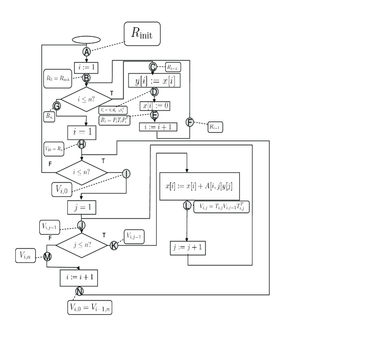
Figure 2: Program annotated with invariants

The annotation is shown in Fig. 2, and relies on the definitions of $S_{i}$, $P_{i}$ and $T_{ij}$ given in (2), (3),and (4). For the sake of simplicity, all invariants are summarized by the corresponding symmetric, semidefinite matrices. Based on our prior discussion, the coherence of these invariants is trivial throughout the program, except (i) during the initialization step (computation of Rinit) and (ii) during the transition from the link denoted $N$ to the link denoted $A$, that is, at the end of the outermost program loop: The ellipsoid ${\mathcal{E}}_{V_{nn}}$ must be contained in the ellipsoid ${\mathcal{E}}_{R_{\mathrm{init}}}$ . For these two properties to hold we pick $R_{\mathrm{init}}$ according to the following observations: As noted earlier, the loop that begins an d ends at the location A performs the following overall matrix iteration (5) on $y$ and $x$. Since $A$ is stable, so is $A_{1}$ and

$$V_{nn}=A_{1}R_{\mathrm{init}}A_{1}^{T}.$$ (9)

Thus we can always find $P>0$ such that

$$A_{1}^{T}PA_{1}-P<0.$$ (10)

Let us define

$$R_{\mathrm{init}}=\alpha P^{-1}$$

where $\alpha$ is a positive scaling parameter. By virtue of Eqs. (10) and (9),

$${\mathcal{E}}V_{nn}\subseteq{\mathcal{E}}_{R_{\mathrm{init}}}$$

whatever the value of $\alpha$. We then pick $\alpha$ to scale ${\mathcal{E}}_{R_{\mathrm{init}}}$ so as to contain all allowed initial values of $x$ and $y$. Assume for example $|x_{i}|\leq 1$, $y_{i}=0$, $i=1,\leq,n$ at program initialization. Then $x^{T}x+y^{T}y\leq n$, that is $x$ and $y$ are contained in the ball ${\mathcal{E}}_{nI}$. Then let $\sigma_{\mathrm{max}}$ be the largest eigenvalue of $P$ satisfying (10). $\sigma_{\mathrm{max}}$ is necessarily positive, and the unit ball ${\mathcal{E}}_{I}$ is included in the ellipsoid ${\mathcal{E}}_{\sigma_{\mathrm{max}}P^{-1}}$ . Let $\alpha=n\sigma_{\mathrm{max}}$. Then the ball ${\mathcal{E}}_{nI}$ is contained in the ellipsoid ${\mathcal{E}}_{\alpha P^{-1}}={\mathcal{E}}_{R_{\mathrm{init}}}$. The annotation process is now complete. To obtain the range over which all variables live in, simply compute the union of all computed ellipsoids above, or compute, say, the minimum volume (or trace) ellipsoid containing all ellipsoids above, or even siompler the minimum-sized ball containing all these ellipsoids.

The following code, written in MATLAB automates this annotation process for a given $A$ matrix

%This code does the documentation automatically...
% for a 2x2 system
%Pick an example
A = [0 1;-0.1 -0.2]
Q=eye(4);
A1 = [zeros(2,2) eye(2);zeros(2,2) A]
%P computation
P = dlyap(A1 ,Q);
%scaling of P
u = max(eig(P));
n = 2;
alpha = 1/u/n/2;
P = alpha*P
%annotation beginning
Rinit = P^(-1);
R0 = Rinit
% i=1
S1 = [eye(2,2) zeros(2,2);zeros(2,2) eye(2,2)];
S1(1,1)=0;S1(1,3)=1;
T1 = S1*R0*S1
P1 = [eye(2,2) zeros(2,2);zeros(2,2) eye(2,2)];
P1(3,3) =0;
R1 = P1*T1*P1
% i=2
S2 = [eye(2,2) zeros(2,2);zeros(2,2) eye(2,2)];
S2(2,2)=0;S2(2,4)=1;
T2 = S2*R1*S2
P2 = [eye(2,2) zeros(2,2);zeros(2,2) eye(2,2)];
P2(4,4) =0;
R2 = P2*T2*P2
V10 = R2
% i=1 j=1
T11 = [eye(2,2) zeros(2,2);zeros(2,2) eye(2,2)];
T11(3,1)= A(1,1);
V11 = T11*V10*T11
% i=1 j=2
T12 = [eye(2,2) zeros(2,2);zeros(2,2) eye(2,2)];
T12(3,2)= A(1,2);
V12 = T12*V11*T12
% i=2 j=1
T21 = [eye(2,2) zeros(2,2);zeros(2,2) eye(2,2)];
T21(4,1)= A(2,1);
V21 = T21*V12*T21
% i=2 j=2
T22 = [eye(2,2) zeros(2,2);zeros(2,2) eye(2,2)];
T22(4,2)= A(2,2);
V22 = T22*V21*T22
%end of loop
% This line checks that indeed, the ellipsoid defined by V22
% is contained in that defined by Rinit;
% The computed eigenvalues ought to be all negative
display( Eigenvalues )
[vV22,eV22]=eig(V22-Rinit)
%quit

Conclusion

This paper has shown one process by which it is possible to carry control system specification certificates down to their software implementation. This process has been shown to be relatively straightforward. We hope to have convinced the reader that this process may be applied to more sophisticated, computer-controlled systems, and that it will eventually lead to the development of more rigorous, yet flexible, embedded software development practices, from its specification down to its operation.

References

- [BCC+03a] B. Blanchet, P. Cousot, R. Cousot., J. Feret, L. Mauborgne, A. Miné, D. Monniaux, and X. Rival. ASTRÉE : A static analyzer for large safety-critical software. Schloß Dagstuhl Seminar 3451, 2–7 November 2003.
- [BCC+03b] B. Blanchet, P. Cousot, R. Cousot, J. Feret, L. Mauborgne, A. Miné, D. Monniaux, and X. Rival. A static analyzer for large safety-critical software. In PLDI. ACM, 2003.
- [BEFB94] S. Boyd, L. El Ghaoui, E. Feron, and V. Balakrishnan. Linear Matrix Inequalities in System and Control Theory, volume 15 of SIAM Studies in Applied Mathematics. SIAM, 1994.
- [Fer04] J. Feret. Static analysis of digital filters. In Proc. 30th ESOP’2004, volume 2986 of Lecture Notes in Computer Science, pages 33–48, Barcelona, 2004. Springer.
- [KV96] A. B. Kurzhanski and I. Valyi. Ellipsoidal Calculus for Estimation and Control. Birkhauser, Boston, 1996.
- [Pel01] D. A. Peled. Software Reliability Methods. Springer, 2001.