What is the probability of connecting two points ?

Abstract

The two-terminal reliability, known as the pair connectedness or connectivity function in percolation theory, may actually be expressed as a product of transfer matrices in which the probability of operation of each link and site is exactly taken into account. When link and site probabilities are $p$ and $\rho$, it obeys an asymptotic power-law behaviour, for which the scaling factor is the transfer matrix’s eigenvalue of largest modulus. The location of the complex zeros of the two-terminal reliability polynomial exhibits structural transitions as $0\leq\rho\leq 1$.

1 Introduction

Since the original work of Moore and Shannon [1], network reliability has been a field devoted to the calculation of the connection probability between different sites of a network constituted by edges (links, bonds) and nodes (vertices, sites), each of them having a probability of operating correctly (the reliability). This field, although mainly developed in an applied background [2], is strongly related to graph theory [3, 4], combinatorics and algebraic structures [5, 6], percolation theory [7, 8], as well as numerous lattice models in statistical physics [9, 10, 11, 12]. For instance, the all-terminal reliability ${\rm Rel}_{A}$, i.e., the probability that all nodes are connected, is derived from the Tutte polynomial, an invariant of the associated graph, when all edges have the same reliability $p$ ($0\leq p\leq 1$). This polynomial appears in the partition function for various Potts models, and has been calculated for several families of graphs [9, 10, 11]; the location of its complex zeros has also been studied [10, 11, 13]. The two-terminal reliability ${\rm Rel}_{2}(s\rightarrow t)$, the probability that a source $s$ and a destination $t$ are connected, is known in percolation theory as the connectivity function or pair connectedness. It has been used in modeling epidemics or fire propagation [7, 8]. This approach is complementary to the effort recently devoted on complex networks, in which the network resilience, i.e., its robustness against link or node failures (sometimes following deliberate attacks) has been studied for ‘scale-free’ random graphs [14].

Exact reliability calculations are known to be very difficult [15], except for series-parallel reducible graphs for which only successive simplifications {$p_{\rm series}=p_{1}\,p_{2}$, $p_{\rm parallel}=p_{1}/\!/p_{2}=p_{1}+p_{2}-p_{1}\,p_{2}$} are needed. Even for planar graphs with identical edge reliabilities $p$ and perfect nodes (i.e., $p_{\rm node}\equiv 1$), their algorithmic complexity has been classified as #P-hard [5, 16]. Yet, the development of Internet traffic makes it important to assess the overall reliability of network connections, when links and nodes may fail.

In this work, we show that for a network represented by an undirected graph $G$, the two-terminal reliability may be expressed as a product of transfer matrices, where individual edge and node reliabilities are exactly taken into account. Such a factorization, already observed for graph colouring polynomials [4, 11], 2D-percolation in square strips [17] or all-terminal reliability polynomials [9, 10], originates with the underlying algebraic structure of the graph. We apply our method to the two examples ($K_{n}$ is the complete graph with $n$ nodes) of figure 1. The $K_{4}$-ladder describes a generic architecture for long-haul connections, while the $K_{3}$-cylinder slightly generalizes the ‘sponge model’ of width three by Seymour and Welsh [18]. When edge and node reliabilities are respectively equal to $p$ and $\rho$, a unique transfer matrix is involved; its largest eigenvalue determines the asymptotic power-law behaviour of reliability as a function of the ladder length. The location of the complex zeros of ${\rm Rel}_{2}(p)$ exhibits striking structure transitions as $\rho$ decreases from one to zero. We illustrate the variety of behaviours for the above-mentioned graphs. For the sake of completeness, we finally give the matrix decomposition for the all-terminal reliability of the $K_{4}$-ladder with arbitrary edge reliabilities (the uniform case has already been treated by Chang and Shrock [9]).

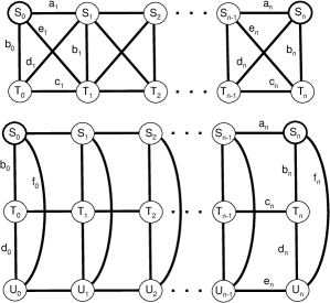
Figure 1: Generic network architectures: (top) $K_{4}$-ladder (bottom) $K_{3}$-cylinder. Links and nodes are identified by their reliabilities: $a_{n}$, $b_{n}$, etc. for links, $S_{n}$, $T_{n}$, and $U_{n}$ for nodes. The source is $S_{0}$, the possible destinations are $S_{n}$, $T_{n}$, or $U_{n}$. A missing link or node’s reliability is simply set to zero.

2 Graph decomposition

The gist of our method is to simplify the graph by removing links of the $n$th (last) elementary cell of the network, namely the edges and nodes indexed by $n$, a procedure called pivotal decomposition or deletion-contraction [5]. If the end terminal $t$ (which can be regarded as perfect) is connected to node $u$ through edge $e$, with respective reliabilities $p_{u}$ and $p_{e}$, then

$${\rm Rel}_{2}(G) = (1-p_{e})\,{\rm Rel}_{2}(G\!\setminus\!e)+p_{e}\,p_{u}\,{\rm Rel}_{2}(G\cdot e)$$ (1)

$$+p_{e}\,(1-p_{u})\,{\rm Rel}_{2}(G\!\setminus\!u),$$

where $G\!\setminus\!e$ and $G\!\setminus\!u$ are the graphs where $e$ or $u$ have been deleted, and $G\cdot e$ the graph where $t$ and $u$ have been merged through the ‘contraction’ of $e$; (1) merely sums probabilities of disjoint events. This procedure, along with standard series-parallel reductions, is repeated for the three (instead of the usual two) secondary graphs in order to take advantage of a structural recursivity of the graph. After a finite number of such reductions, we get replicas of the original graph, albeit with one less elementary cell and with the $(n-1)$th cell’s edge and node reliabilities possibly renormalized by those of the $n$th cell, or set to either zero or one. In order to ensure the existence of a recursion relation, the graph structure must be closed under successive applications of (1); it may initially require the use of extra edges with symbolic reliabilities, so that all nodes of an elementary cell are connected pair-wise, even if such links do not exist in the graph under consideration. At this point, a recursion hypothesis is needed, giving for instance ${\rm Rel}_{2}(S_{0}\!\rightarrow\!S_{n})$ as a sum over specific polynomials in the reliabilities indexed by $n$; these are often obvious from the $n=2$ value. Going from $n-1$ to $n$ provides the transfer matrix linking the prefactors of the polynomials, because ${\rm Rel}_{2}$ is an affine function of each component reliability; the (often trivial) $n=1$ case serves as the initial condition of the recurrence.

3 Application to the $K_{4}$-ladder

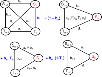
Figure 2: First step of the pivotal decomposition : the removal of edge $b_{n}$. Three structurally identical, secondary graphs are obtained.

Let us first illustrate this method by calculating ${\mathcal{R}}_{n}={\rm Rel}_{2}(S_{0}\!\rightarrow\!S_{n})$ for the $K_{4}$-ladder (top of figure 1). Following the guidelines of the preceding section, we first consider $b_{n}$ for deletion as detailed in figure 2. Note that the three secondary graphs have essentially the same structure. The renewed application of (1) leads to two families of contributions. The first one is a sum of ${\mathcal{R}}_{n-1}$-like terms with prefactors, in which the ‘old’ $a_{n-1}$, …, $T_{n-1}$ are renormalized by one or more of the ‘new’ $a_{n}$, …, $T_{n}$. The second one is a sum of ${\rm Rel}_{2}(S_{0}\!\rightarrow\!T_{n-1})$-like terms. There is no need for coupled recursion relations for the two destinations $S_{n}$ and $T_{n}$, since they are essentially identical through the permutations $a_{n}\!\leftrightarrow\!e_{n}$, $c_{n}\!\leftrightarrow\!d_{n}$, and $S_{n}\!\leftrightarrow\!T_{n}$. ${\mathcal{R}}_{n}$ may be expressed as the sum of five polynomials in $a_{n}$, …, $T_{n}$ (see below). The five prefactors at step $n$ are obtained from those at step $n-1$ by a recursion relation which translates as a $5\times 5$ transfer matrix (such calculations are routinely performed by mathematical software). The value of ${\mathcal{R}}_{1}$ leads to

$${\mathcal{R}}_{n} = (1\;0\;0\;0\;0)\,M_{n}\,M_{n-1}\,\cdots M_{1}\,M_{0}\,\left(\begin{array}[]{c}1\\ 0\\ 0\\ 0\\ 0\end{array}\right),$$ (7)

where $M_{i}$’s coefficients $M_{kl}$ are ($\overline{x}\equiv 1-x$)

$$M_{11} = (a_{i}+b_{i}\,e_{i}\,T_{i}-a_{i}\,b_{i}\,e_{i}\,T_{i})\,S_{i},$$ (8a)

$$M_{12} = (d_{i}+b_{i}\,c_{i}\,T_{i}-d_{i}\,b_{i}\,c_{i}\,T_{i})\,S_{i},$$ (8b)

$$M_{13} = a_{i}\,d_{i}\,S_{i}+b_{i}\,(\chi_{i}+c_{i}\,e_{i})\,S_{i}\,T_{i},$$ (8c)

$$M_{14} = -M_{44}=a_{i}\,\,e_{i}\,M_{42},$$ (8d)

$$M_{15} = -M_{45}=c_{i}\,\,d_{i}\,M_{41},$$ (8e)

$$M_{21} = (e_{i}+b_{i}\,a_{i}\,S_{i}-e_{i}\,b_{i}\,a_{i}\,S_{i})\,T_{i},$$ (8f)

$$M_{22} = (c_{i}+b_{i}\,d_{i}\,S_{i}-c_{i}\,b_{i}\,d_{i}\,S_{i})\,T_{i},$$ (8g)

$$M_{23} = c_{i}\,e_{i}\,T_{i}+b_{i}\,(\chi_{i}+a_{i}\,d_{i})\,S_{i}\,T_{i},$$ (8h)

$$M_{24} = -M_{54}=a_{i}\,\,e_{i}\,M_{52},$$ (8i)

$$M_{25} = -M_{55}=c_{i}\,\,d_{i}\,M_{51},$$ (8j)

$$M_{31} = -(a_{i}\,b_{i}+a_{i}\,e_{i}+b_{i}\,e_{i}-2\,a_{i}\,b_{i}\,e_{i})\,S_{i}\,T_{i},$$ (8k)

$$M_{32} = -(b_{i}\,c_{i}+b_{i}\,d_{i}+c_{i}\,d_{i}-2\,b_{i}\,c_{i}\,d_{i})\,S_{i}\,T_{i},$$ (8l)

$$M_{33} = \left((1-2\,b_{i})\,\chi_{i}-b_{i}\,(c_{i}\,e_{i}+a_{i}\,d_{i})\right)\,S_{i}\,T_{i},$$ (8m)

$$M_{34} = -M_{14}-M_{24},$$ (8n)

$$M_{35} = -M_{15}-M_{25},$$ (8o)

$$M_{41} = \overline{a_{i}}\,\overline{b_{i}}\,e_{i}\,S_{i}\,T_{i},$$ (8p)

$$M_{42} = \overline{b_{i}}\,c_{i}\,\overline{d_{i}}\,S_{i}\,T_{i},$$ (8q)

$$M_{43} = \overline{b_{i}}\,(\chi_{i}+c_{i}\,e_{i})\,S_{i}\,T_{i},$$ (8r)

$$M_{51} = a_{i}\,\overline{b_{i}}\,\overline{e_{i}}\,S_{i}\,T_{i},$$ (8s)

$$M_{52} = \overline{b_{i}}\,\overline{c_{i}}\,d_{i}\,S_{i}\,T_{i},$$ (8t)

$$M_{53} = \overline{b_{i}}(\chi_{i}+a_{i}\,d_{i})\,S_{i}\,T_{i},$$ (8u)

with $\chi_{i}=\overline{a_{i}}\,\overline{c_{i}}\,d_{i}\,e_{i}+a_{i}\,c_{i}\,\overline{d_{i}}\,\overline{e_{i}}-a_{i}\,c_{i}\,d_{i}\,e_{i}$. In the $n=0$ case, $a_{0}=1$ and $c_{0}=d_{0}=e_{0}=0$. The five above-mentioned polynomials are actually given by the first row of $M_{n}$. ${\rm Rel}_{2}(S_{0}\!\rightarrow\!T_{n})$ is given by (7) if the left vector is $(0\;1\;0\;0\;0)$. We have here another useful instance of a product of random matrices [19].

The case of identical reliabilities $a_{i}=\cdots=e_{i}=p$ (unless $i=0$, see the restriction above) and $S_{i}=T_{i}=\rho$ is worth investigating, since only the $n$th power of a unique matrix needs be taken. Because of the recursion relation between successive values of ${\mathcal{R}}_{n}$, the generating function ${\mathcal{G}}(z)=\sum_{n=0}^{\infty}\,{\mathcal{R}}_{n}\,z^{n}$ is a rational fraction of $z$. Its denominator ${\mathcal{D}}(z)$ is derived from the characteristic polynomial of the transfer matrix, taken at $1/z$. The numerator of ${\mathcal{G}}(z)$ is then deduced from the computed first terms of the ${\mathcal{G}}(z)\,{\mathcal{D}}(z)$’s expansion. The final result reads:

$${\mathcal{G}}(z) = \frac{1}{2}\,\rho\,(1-p\,\rho)+\frac{{\mathcal{N}}(z)}{{\mathcal{D}}(z)},$$ (8i)

$${\mathcal{N}}(z) = \frac{1}{2}\,\rho\,(1+p\,\rho)$$ (8j)

$$-\frac{1}{2}\,p^{2}\,\rho^{3}\,(2-10\,p+13\,p^{2}-4\,p^{3}-p^{3}\,\rho)\,z$$

$$+(1-p)^{2}\,p^{5}\,(2-4\,p+p^{2})\,(1-\rho)\,\rho^{5}\,z^{2},$$

$${\mathcal{D}}(z) = 1-p\,\rho\,\left(2+4\,p\,\rho-14\,p^{2}\,\rho+13\,p^{3}\,\rho-4\,p^{4}\,\rho\right)\,z$$ (8k)

$$+2\,\left(1-p\right)\,p^{3}\,{\rho}^{3}\,\left(2-7\,p+4\,p^{2}+7\,p^{2}\,\rho\right.$$

$$\left.\hskip 71.13188pt-10\,p^{3}\,\rho+5\,p^{4}\,\rho-p^{5}\,\rho\right)\,z^{2}$$

$$-4\,\left(2-p\right)\,{\left(1-p\right)}^{3}\,p^{6}\,\left(1-\rho\right)\,{\rho}^{5}\,z^{3}.$$

Equations (8i–8k) are simpler for perfect nodes, because the denominator is of degree 2 in $z$; a partial fraction decomposition provides

$${\mathcal{R}}_{n} = \frac{1-p}{2}\,\delta_{n,0}+a_{+}\,\lambda_{+}^{n}+a_{-}\,\lambda_{-}^{n},$$ (8l)

$$\lambda_{\pm} = \frac{p}{2}\,\left[2+4\,p-14\,p^{2}+13\,p^{3}-4\,p^{4}\pm\sqrt{{\mathcal{A}}}\right],$$ (8m)

$$a_{\pm} = \frac{1+p}{4}\pm\frac{2+2\,p+10\,p^{2}-27\,p^{3}+19\,p^{4}-4\,p^{5}}{4\,\sqrt{{\mathcal{A}}}},$$

$${\mathcal{A}} = 4+32\,p^{2}-204\,p^{3}+452\,p^{4}-516\,p^{5}$$ (8o)

$$+329\,p^{6}-112\,p^{7}+16\,p^{8}.$$

As $n$ grows, ${\mathcal{R}}_{n}\approx a_{+}\,\lambda_{+}^{n}$: the two-terminal reliability exhibits a power-law behaviour, the scaling factor being $\lambda_{+}$, the eigenvalue of largest modulus. Alternatively, ${\mathcal{R}}_{n}\sim\exp(-n/\xi)$, where $\xi=-1/\ln(\lambda_{+})$ is the correlation length of percolation theory [7].

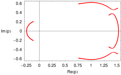
Figure 3: Location of the complex zeros of the two-terminal reliability polynomial ${\mathcal{R}}_{n}(p,\rho)$ for $n=150$ and $\rho=1$.

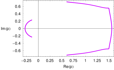
Figure 4: Same as figure 3, with $\rho=0.8$.

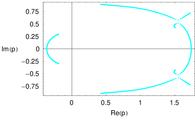
Figure 5: Same as figure 3, with $\rho=0.5$.

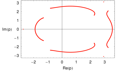
Figure 6: Same as figure 3, with $\rho=0.01$.

The location of the zeros of ${\rm Rel}_{2}(p)$ in the complex plane is also worth investigating. The situation differs from that for chromatic [4, 11] and all-terminal polynomials [9], because ${\rm Rel}_{2}(p)$ is not a graph invariant. However, the node reliability $\rho$ is an extra parameter that has a deep impact on the curves to which the zeros of ${\rm Rel}_{2}(p)$ converge as $n\rightarrow\infty$. The critical values of $\rho$ at which shape transitions occur may be deduced [20] from the three roots of ${\mathcal{D}}(1/z)$. The straightforward but tedious procedures used to determine these values, along with a few asymptotic expansions as $\rho\to 0$, are outlined in the Appendix (they are also applied to the $K_{3}$-cylinder configuration). We limit ourselves to the final results in the following sections.

A sample of the richness of behaviour is displayed in figures 3–6 for the $K_{4}$-ladder and decreasing values of $\rho$. We initially observe four well-separated ‘curves’ that merge into two when $\rho$ is exactly equal to 0.8 (see figure 4) and separate again. When $\rho$ further decreases, other isolated zeros appear, as in figure 6. These zeros occur in pairs, the separation of which vanishes exponentially with $n$, and converge to roots of the algebraic equation

$$0 = 2+2\,\rho+4\,(3\,\rho+1)\,\rho\,p-(40\,\rho+11)\,\rho\,p^{2}$$ (8p)

$$+(45\,\rho+4)\,\rho\,p^{3}-20\,\rho^{2}\,p^{4}+3\,\rho^{2}\,p^{5}\,.$$

Equation (8p) is obtained by ensuring that ${\mathcal{N}}(z)$ and ${\mathcal{D}}(z)$ have a common root. The true limiting isolated points are such that this root is the eigenvalue of greatest complex modulus at the given $p$ and $\rho$. Actually, the triplet of figure 6 appears only when $\rho<\rho_{{\rm c}_{1}}\approx 0.175221381869$, where $\rho_{{\rm c}_{1}}$ is a solution of (see the Appendix)

$$0 = -32768-198656\,\rho+3990544\,{\rho}^{2}-12843528\,{\rho}^{3}$$ (8q)

$$+16258037\,{\rho}^{4}-6757568\,{\rho}^{5}-2015436\,{\rho}^{6}-575540\,{\rho}^{7}$$

$$+4636356\,{\rho}^{8}-3082436\,{\rho}^{9}+624640\,{\rho}^{10}\,,$$

whereas the associated $p_{{\rm c}_{1}}\approx-0.604692601721$ is a solution of

$$0 = 40-364\,p+1064\,p^{2}-700\,p^{3}-1946\,p^{4}+4296\,p^{5}$$ (8r)

$$-3465\,p^{6}+1074\,p^{7}+146\,p^{8}-176\,p^{9}+32\,p^{10}\,.$$

If $\rho_{{\rm c}_{1}}<\rho<\rho_{{\rm c}_{2}}\approx 0.406657811123$ (the algebraic equation satisfied by $\rho_{{\rm c}_{2}}$ is actually of degree 65 in $\rho$), only the two rightmost isolated points are present.

The leftmost isolated point, located on the real negative axis, is asymptotically given by $-(2\,\rho)^{-1/3}+25/24+\Or(\rho^{1/3})$; for the other two, $\rho$ must be replaced by $\rho\,e^{\pm 2\,\rmi\,\pi}$. By contrast, the algebraic curves’ asymptotic limit is a circle of radius $(2\,\rho)^{-1/4}$ centred at $(27/32,0)$, demonstrating a different power-law behaviour with $\rho$. Finally, a third critical value $\rho_{{\rm c}_{3}}\approx 0.49137068$ also appears, for which we have not been able to find the defining algebraic equation satisfied by $\rho$ (its degree is likely to be large); at this value, there is an asymptotic (anti-)crossing of the curves in the vicinity of $p\approx 1.55533445+\rmi\,0.55314582$.

4 $K_{3}$-cylinder

In the second architecture of figure 1, $S_{0}$ is still the source while $S_{n}$, $T_{n}$, and $U_{n}$ are the three possible destinations (the last two are equivalent through a permutation of variables). The crucial point is to take all $f_{i}\neq 0$, because in the successive applications of (1), the merging of nodes entails a secondary graph in which $S_{n-1}$ and $U_{n-1}$ are connected. As mentioned above, the dummy — with respect to the Manhattan-like strip — link $f_{n}$ between $S_{n}$ and $U_{n}$ must therefore be present right at the start; this allows us to unveil the coupled recursion relations between the source and all the destinations. Each source-destination reliability is a sum of eight polynomials in reliabilities indexed by $n$. This could lead to $24\times 24$ transfer matrices $\widetilde{M}_{i}$. However, several rows of these matrices, if not identical, are linearly dependent; rearrangements of terms actually reduce their size to $13\times 13$, even when $f_{i}=0$.

The final result reads

$${\widetilde{\mathcal{R}}}_{n} = {\mathbf{v}}_{L}\,\widetilde{M}_{n}\,\widetilde{M}_{n-1}\,\cdots\widetilde{M}_{1}\,\widetilde{M}_{0}\,{\mathbf{v}}_{R},$$ (8s)

where ${\mathbf{v}_{R}}$ is the column vector defined by $({\mathbf{v}_{R}})_{k}=\delta_{k1}$ for $1\leq k\leq 13$ (using the Kronecker notation: $\delta_{kl}$ is equal to 1 if $k=l$ and 0 if $k\neq l$), and ${\mathbf{v}_{L}}$ is a row vector which depends on the destination: $\left({\mathbf{v}}_{S_{n}}\right)_{k}=\delta_{1k}$, $\left({\mathbf{v}}_{T_{n}}\right)_{k}=\delta_{2k}$, and $\left({\mathbf{v}}_{U_{n}}\right)_{k}=\delta_{3k}$. The matrix elements are much lengthier than in (8a–8u), and are given in the Appendix for the sake of completeness.

4.1 $f_{i}=0$

Following the procedure outlined in the preceding section, we can compute the new generating function. For perfect nodes, $\widetilde{{\mathcal{G}}}(S_{0}\!\rightarrow\!U_{n})$ is given by $\widetilde{{\mathcal{N}}}/(\widetilde{{\mathcal{D}}}_{1}\,\widetilde{{\mathcal{D}}}_{2})$:

$$\widetilde{{\mathcal{N}}} = p^{2}-\left(1-p\right)\,p^{4}\,\left(3+3\,p-4\,p^{2}\right)\,z$$ (8t)

$$\hskip-28.45274pt+{\left(1-p\right)}^{3}\,p^{6}\,\left(2+11\,p-3\,p^{2}-2\,p^{3}\right)\,z^{2}$$

$$\hskip-28.45274pt+{\left(1-p\right)}^{3}\,p^{8}\,\left(2-4\,p+3\,p^{2}+11\,p^{3}-13\,p^{4}+3\,p^{5}\right)\,z^{3}$$

$$\hskip-28.45274pt-{\left(1-p\right)}^{4}\,p^{10}\,\left(3+6\,p-12\,p^{2}+10\,p^{3}-10\,p^{4}+4\,p^{5}\right)\,z^{4}$$

$$\hskip-28.45274pt+{\left(1-p\right)}^{6}\,p^{12}\,\left(1+8\,p-p^{2}-5\,p^{3}-p^{4}+p^{5}\right)\,z^{5}$$

$$\hskip-28.45274pt-{\left(1-p\right)}^{8}\,p^{15}\,\left(2+5\,p-4\,p^{2}\right)\,z^{6}+{\left(1-p\right)}^{10}\,p^{18}\,z^{7},$$

$$\widetilde{{\mathcal{D}}}_{1} = 1-\left(1-p^{2}\right)\,p\,\left(1+p-p^{2}\right)\,z$$ (8u)

$$\hskip-28.45274pt+{\left(1-p\right)}^{2}\,p^{3}\,\left(1+p+p^{2}-2\,p^{3}\right)\,z^{2}-{\left(1-p\right)}^{4}\,p^{6}\,z^{3},$$

$$\widetilde{{\mathcal{D}}}_{2} = 1-p\,\left(2+2\,p+p^{2}-9\,p^{3}+5\,p^{4}\right)\,z$$ (8v)

$$+\left(1-p\right)\,p^{2}\,\left(1+5\,p+5\,p^{2}-6\,p^{3}-15\,p^{4}\right.$$

$$\left.\hskip 62.59596pt+13\,p^{5}+p^{6}-2\,p^{7}\right)\,z^{2}$$

$$-{\left(1-p\right)}^{2}\,p^{4}\,\left(2+6\,p+6\,p^{2}-26\,p^{3}+17\,p^{4}\right.$$

$$\left.\hskip 62.59596pt-18\,p^{5}+27\,p^{6}-16\,p^{7}+3\,p^{8}\right)\,z^{3}$$

$$+{\left(1-p\right)}^{4}\,p^{6}\,\left(1+6\,p+4\,p^{2}-p^{3}-17\,p^{4}\right.$$

$$\left.\hskip 62.59596pt+9\,p^{5}+3\,p^{6}-2\,p^{7}\right)\,z^{4}$$

$$-{\left(1-p\right)}^{6}\,p^{9}\,\left(2+4\,p+p^{2}-7\,p^{3}+3\,p^{4}\right)\,z^{5}$$

$$+{\left(1-p\right)}^{8}\,p^{12}\,z^{6}.$$

When $\rho\neq 1$, the degrees of $\widetilde{{\mathcal{N}}}$, $\widetilde{{\mathcal{D}}}_{1}$, $\widetilde{{\mathcal{D}}}_{2}$ are still 7, 3 and 6, respectively; their expressions are only lengthier.

The eigenvalue of greatest modulus $\lambda_{\rm max}$ involved in the asymptotic power-law behaviour obeys $\widetilde{{\mathcal{D}}}_{2}(1/\lambda_{\rm max})=0$. The degree of the denominator leads us to expect that the ‘width’ of the network should drastically affect the size of the transfer matrices.

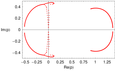
Figure 7: Complex zeros of the two-terminal reliability polynomial for the $K_{3}$-cylinder, $f_{i}=0$, $n=100$ and $\rho=1$.

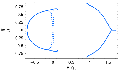
Figure 8: Same as figure 7, with $\rho=0.6$.

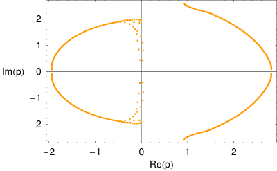
Figure 9: Same as figure 7, with $\rho=0.1$.

The associated complex zeros are displayed for various values of $\rho$ in figures 7–9. The overall structure is more complicated than that for the $K_{4}$-ladder, but some features are quite similar.

A segment of the real axis appears as a limit curve when $0.4202958<\rho<0.8092264$. These critical values obey different criteria. Indeed, the higher one (with the associated critical, real $p\approx 1.53039659$) occurs when two complex roots of $\widetilde{{\mathcal{D}}}_{2}(z)$ have the same (lowest) modulus as a real negative root of $\widetilde{{\mathcal{D}}}_{1}(z)$. By contrast, the lower critical value 0.4202958 appears when $\widetilde{{\mathcal{D}}}_{2}(z)$ exhibits two complex roots and a real positive root with the same modulus (the critical $p$ is about 1.8363587).

What happens when $\rho\to 0$ ? The outermost parts of the curves tend asymptotically to a circle of radius $\displaystyle\frac{\left(5-\sqrt{17}\right)^{1/4}}{\sqrt{2\,\rho}}$, i.e., approximately $\displaystyle\frac{0.684261}{\sqrt{\rho}}$. The closed curve on the left survives. For instance, a triple point $p_{t}$ goes asymptotically as $\displaystyle\pm\frac{\rmi\,a}{\sqrt{\rho}}+b$, with $a\approx 0.4610389$ and $b\approx-0.08457522$ ($a^{2}$ is a root of a polynomial of degree 10, and $b$ is a rational fraction of $a$). From each of these points, two curves head back to the origin. One of them crosses the imaginary axis at $\displaystyle p\sim\pm\frac{\rmi\,a^{\prime}}{\sqrt{\rho}}$, with $a^{\prime}\approx 0.33529987$ (${a^{\prime}}^{2}$ is actually the root of a polynomial of degree 17).

4.2 $f_{i}\neq 0$

In this case, the generating function $\widetilde{{\mathcal{G}}^{\prime}}(S_{0}\!\rightarrow\!U_{n})$ is now equal to $\widetilde{{\mathcal{N}}^{\prime}}/(\widetilde{{\mathcal{D}}^{\prime}}_{1}\,\widetilde{{\mathcal{D}}^{\prime}}_{2})$, where for perfect nodes

$$\widetilde{{\mathcal{N}}^{\prime}} = p\,(1+p-p^{2})$$ (8w)

$$-(2-p)\,{(1-p)}^{2}\,p^{3}\,(1+p)\,(1+3\,p-3\,p^{2})\,z$$

$$+{(1-p)}^{5}\,p^{5}\,(1+10\,p+8\,p^{2}-5\,p^{3}-2\,p^{4})\,z^{2}$$

$$-{(1-p)}^{6}\,p^{8}\,(3+8\,p-25\,p^{2}+9\,p^{3}+4\,p^{4}-p^{5})\,z^{3}$$

$$+{(1-p)}^{8}\,p^{11}\,(1-2\,p)\,(3+3\,p-7\,p^{2}+2\,p^{3})\,z^{4}$$

$$-{(1-p)}^{11}\,p^{14}\,(1-3\,p+p^{2})\,z^{5},$$

$$\widetilde{{\mathcal{D}}^{\prime}}_{1} = 1-{\left(1-p\right)}^{2}\,p\,\left(1+p\right)\,\left(1+p-p^{2}\right)\,z$$ (8x)

$$+{\left(1-p\right)}^{4}\,p^{3}\,\left(1+p+p^{2}-2\,p^{3}\right)\,z^{2}$$

$$-{\left(1-p\right)}^{7}\,p^{6}\,z^{3},$$

$$\widetilde{{\mathcal{D}}^{\prime}}_{2} = 1-p\,(1+3\,p+4\,p^{2}-23\,p^{3}+23\,p^{4}-7\,p^{5})\,z$$ (8y)

$$+{(1-p)}^{2}\,p^{3}\,(1+6\,p+2\,p^{2}-9\,p^{3}$$

$$\hskip 62.59596pt-8\,p^{4}+16\,p^{5}-6\,p^{6})\,z^{2}$$

$$-{(1-p)}^{4}\,p^{6}\,(2+4\,p+p^{2}-15\,p^{3}+12\,p^{4}-3\,p^{5})\,z^{3}$$

$$+{(1-p)}^{7}\,p^{9}\,z^{4}.$$

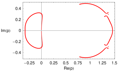
Figure 10: Complex zeros of the two-terminal reliability polynomial for the $K_{3}$-cylinder, $f_{i}\neq 0$, $n=100$ and $\rho=1$.

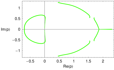
Figure 11: Same as figure 10, with $\rho=0.3$.

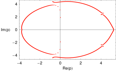
Figure 12: Same as figure 10, with $\rho=0.01$.

Note that $\widetilde{{\mathcal{D}}^{\prime}}_{2}$ is of degree 4 in $z$ (even when $\rho\neq 1$), so that a complete analytical solution for the two-terminal reliability could be obtained — but would be very cumbersome.

The location of complex zeros are displayed in figures 10–12. Critical values of different nature occur in this case. Two isolated zeros exist as long as $0.3633122889<\rho\leq 1$. They do not survive in the $\rho\to 0$ limit, in contrast with the $K_{4}$ case. For $\rho\approx 0.3633122889$, they merge with a continuous curve at $p\approx 1.466816\pm\rmi\,0.5823927$. For these isolated points, the relevant $p$ and $\rho$ obey the polynomial constraint

$$0 = -2\,\left(1-2\,p\right)\,\left(1+5\,p-4\,p^{2}\right)$$ (8z)

$$-p\,\left(1+39\,p-172\,p^{2}+316\,p^{3}-230\,p^{4}+56\,p^{5}\right)\,\rho$$

$$+p^{2}\,\left(12+42\,p-416\,p^{2}+947\,p^{3}-899\,p^{4}\right.$$

$$\left.\hskip 28.45274pt+382\,p^{5}-60\,p^{6}\right)\,{\rho}^{2}$$

$$+p^{3}\,\left(27-45\,p+33\,p^{2}-90\,p^{3}+135\,p^{4}\right.$$

$$\left.\hskip 28.45274pt-77\,p^{5}+15\,p^{6}\right)\,{\rho}^{3},$$

the origin of which is similar to that of (8p).

Another feature is the segment on the real axis (see figure 11) which occurs when $0.016301418<\rho<0.83140245$. These two critical values are actually solutions of a polynomial in $\rho$ of degree 95, and the associated critical $p$’s, namely 1.60638989 and 4.56013168, are also roots of a polynomial in $p$ of degree 95. These transitions occur when the equation $\widetilde{{\mathcal{D}}^{\prime}}_{2}(z)=0$ has a double, real (negative) root, the opposite of which is also a root.

As in the preceding subsection, the global structure expands as $\rho\to 0$. The outer curves tend asymptotically to a circle of radius $\displaystyle\frac{1}{7^{1/5}\,\rho^{2/5}}\approx 0.677611\,\rho^{-2/5}$. The closed curve on the left also survives (see figure 12). Here again, it crosses the imaginary axis asymptotically at $\displaystyle p\sim\pm\rmi\,\left(\frac{10^{-1/6}}{\rho^{1/3}}-\frac{3}{5\,\sqrt{10}}\right)$.

5 Transfer matrices for the all-terminal reliability ${\rm Rel}_{A}$

Nodes may be viewed as perfect in this case since the node reliabilities can be factored out, and simpler calculations may be done because (1) has one less term. For the $K_{4}$-ladder, the transfer matrix is $2\times 2$:

$${\rm Rel}_{A}(n)=(1\,0)\;\widehat{M}_{n}\;\cdots\;\widehat{M}_{n-1}\;\widehat{M}_{0}\left(\begin{array}[]{c}1\\ 0\end{array}\right);$$ (8aa)

The matrix elements $(\widehat{M}_{i})_{kl}$ of $\widehat{M}_{i}$ are ($\overline{x}\equiv 1-x$)

$$(\widehat{M}_{i})_{11} = [(a_{i}+e_{i})\,(c_{i}+d_{i})-2\,a_{i}\,c_{i}\,d_{i}\,e_{i}]\,\overline{b_{i}}$$ (8ab)

$$+[(a_{i}/\!/e_{i})+(c_{i}/\!/d_{i})]\,b_{i},$$

$$(\widehat{M}_{i})_{12} = a_{i}\,c_{i}\,d_{i}\,e_{i}\,[\frac{1}{a_{i}}+\frac{1}{c_{i}}+\frac{1}{d_{i}}+\frac{1}{e_{i}}-3]\,\overline{b_{i}}$$ (8ac)

$$+[(a_{i}/\!/e_{i})\,(c_{i}/\!/d_{i})]\,b_{i},$$

$$(\widehat{M}_{i})_{21} = [(a_{i}/\!/c_{i})+(d_{i}/\!/e_{i})-2\,(a_{i}\,e_{i}/\!/c_{i}\,d_{i})]\,\overline{b_{i}}$$ (8ad)

$$-(\widehat{M}_{i})_{11},$$

$$(\widehat{M}_{i})_{22} = (c_{i}+d_{i}-2\,c_{i}\,d_{i})\,(a_{i}+e_{i}-2\,a_{i}\,e_{i})\,\overline{b_{i}}$$ (8ae)

$$-(\widehat{M}_{i})_{12};$$

in $\widehat{M}_{0}$, $a_{0}=1$ and $c_{0}=d_{0}=e_{0}=0$. This is a special case of a multivariate Tutte polynomial [21]. If $a_{i}=\cdots=e_{i}\equiv p$ ($0\leq i\leq n$), we recover Chang and Shrock’s result (appendix 4.2 of [9]) $\widehat{{\mathcal{G}}}_{A}(z)=\widehat{{\mathcal{N}}}_{A}(z)/\widehat{{\mathcal{D}}}_{A}(z)$ with

$$\widehat{{\mathcal{N}}}_{A}(z) = p+p^{3}\,(1-p)\,(4-3\,p)\,z,$$ (8af)

$$\widehat{{\mathcal{D}}}_{A}(z) = 1-p^{2}\,\left(12-26\,p+21\,p^{2}-6\,p^{3}\right)\,z$$ (8ag)

$$+2\,p^{5}\,{\left(1-p\right)}^{3}\,\left(2-p\right)\,z^{2}.$$

The asymptotic power-law scaling factor is controlled by $\zeta_{+}=\frac{1}{2}\,p^{2}\,(12-26\,p+21\,p^{2}-6\,p^{3}+\sqrt{{\mathcal{B}}})$ with ${\mathcal{B}}=144-640\,p+1236\,p^{2}-1308\,p^{3}+793\,p^{4}-260\,p^{5}+36\,p^{6}$.

6 Conclusion and perspectives

The two-terminal reliability of undirected networks may be expressed by a product of transfer matrices, in which each edge and node reliability is exactly taken into account. This result is easily extended to the all-terminal reliability with nonuniform links, as well as to directed graphs. We can now go beyond series-parallel simplifications and look for new (wider) families of exactly solvable, meshed architectures that may be useful for general reliability studies (as building blocks for more complex networks), for the enumeration of self-avoiding walks on lattices, and for percolation with imperfect bonds and sites. Since the true generating function is itself a rational fraction, Padé approximants should provide efficient upper or lower bounds for these studies. Moreover, individual reliabilities can be viewed as average values of random variables. Having access to each edge or node allows the introduction of disorder or correlations in calculations. The location of complex zeros of the two-terminal reliability polynomials exhibits numerous structure transitions, with the possible occurrence of isolated points, convergence to segments of the real axis, and also an expansion from the origin as $\rho$ goes to 0 which obeys power-law behaviours with rational exponents which may differ strongly for seemingly not too dissimilar graphs. All critical values of the node reliability are actually algebraic values. Finally, in a more applied perspective, let us mention that the failure frequency $\nu$ of a given connection is another important performance index of networks. If equipment $i$ with reliability $p_{i}$ has a failure rate $\lambda_{i}$, $\nu=\sum_{i}\,\lambda_{i}\,p_{i}\,\partial{\rm Rel}_{2}/\partial p_{i}$. The matrix factorization makes the calculation straightforward, since each $p_{i}$ appears in one transfer matrix only.

Appendix A A few recipes on the determination of the complex zeros of two-variate polynomials

Our method relies on well-known results for the zeros of recursively defined one-parameter polynomials [4, 9, 11, 20]. Since we are dealing here with two-variate ($p$,$\rho$) polynomials, let us outline the procedure used to obtain the figures, the critical values, and the asymptotic expansions given in the text.

A.1 Determination of the two-variate polynomial

As shown by many published studies, the convergence of the zeros to limiting sets of algebraic curves is already apparent for $n$ roughly equal to 50. To be on the safe side, we calculated these polynomials for $n=100$ or $n=150$ in order to (i) be very close to the asymptotic limit (ii) get a good sampling of the zeros, since — especially in the small-$\rho$ limit — they are not uniformly distributed over the asymptotic curves when $n\to\infty$ (see figures 7–9 and 12).

We have calculated these polynomials using Mathematica and recursion relations based on the denominator of the generating function. If

$${\mathcal{D}}(z)=1+b_{1}(p,\rho)\,z+b_{2}(p,\rho)\,z^{2}+\cdots+b_{m}(p,\rho)\,z^{m}\,,$$ (8ah)

then

$${\rm Rel}_{2}^{(n)}=-b_{1}(p,\rho)\,{\rm Rel}_{2}^{(n-1)}-b_{2}(p,\rho)\,{\rm Rel}_{2}^{(n-2)}-\cdots-b_{m}(p,\rho)\,{\rm Rel}_{2}^{(n-m)}\,.$$ (8ai)

Knowledge of the first $m$ polynomials deduced from the generating function allows the quick determination of ${\rm Rel}_{2}^{(n)}$ for a given $\rho$. $\rho$ has not been kept as a parameter because of the explosion in the number of terms, but has been given rational values in order to prevent numerical errors; this gives polynomials with integral coefficients that may be very large (hundreds of digits sometimes). Their zeros have been obtained using Mathematica’s routine NSolve, the accuracy of which must be set accordingly (higher than hundreds of digits).

A.2 Limiting curves and isolated zeros

The zeros of recursively defined (one-parameter) polynomials mostly tend to aggregate close to curves such as (at least) two eigenvalues have the same modulus (the largest one for all the eigenvalues). Assuming that the ratio of the two eigenvalues is equal to $e^{{\rm i}\,\theta}$, we can write

$${\mathcal{D}}(z)=(1-\zeta\,e^{{\rm i}\,\theta/2}\,z)\,(1-\zeta\,e^{-{\rm i}\,\theta/2}\,z)\,(1-\widetilde{b}_{1}\,z-\cdots-\widetilde{b}_{m-2}\,z^{m-2}),$$ (8aj)

which must be compared with (8ah). Elimination of $\zeta$ and the $\widetilde{b}_{k}$’s leads to a (polynomial) relationship between $p$, $\rho$ and even powers of $t=\cos(\theta/2)$. Replacing $t$ by the more practical $T=\cos\theta$ gives a polynomial constraint ${\mathcal{C}}(p,\rho,T)=0$. However, the true limiting curves are defined by only a subset of this constraint’s many solutions for a given $\rho$ and $T$ ranging from -1 to +1, because $|\zeta|$ must be the largest. In this context, it does no harm to investigate special points of these curves.

A.2.1 Double roots of ${\mathcal{D}}(z)=0$

In our case studies the endpoints of the limiting curves are such that both roots are equal ($\theta=0$ or equivalently $T=+1$): they are thus obtained from a subset of the solutions of ${\widehat{\mathcal{C}}}(p,\rho)={\mathcal{C}}(p,\rho,T=+1)=0$. For the $K_{4}$-ladder with $\rho=1$, this leads to

$$0 = (2-p)^{2}\,(1-p)^{4}\,(1-p+p^{2})^{2}\,$$ (8ak)

$$(4+32\,p^{2}-204\,p^{3}+452\,p^{4}-516\,p^{5}+329\,p^{6}-112\,p^{7}+16\,p^{8})\,$$

which gives the true endpoints of figure 3: $-0.1175415\pm{\rm i}\,0.2041183$, $0.7609223\pm{\rm i}\,0.5877642$, $1.343654\pm{\rm i}\,0.3456238$, and $1.512965\pm{\rm i}\,0.4931547$ (all the solutions are actually roots of the polynomial of degree 8). A quicker way to find these endpoints is to investigate when ${\mathcal{D}}(z)$ and $\displaystyle\frac{\partial{\mathcal{D}}(z)}{\partial z}$ are both equal to zero. Elimination of $z$ from these two equations leads to the desired ${\widehat{\mathcal{C}}}(p,\rho)$, or more accurately, to a product of two-variate polynomials. Confrontation with numerical estimates of the zeros allows to remove spurious solutions.

A.2.2 Opposite roots of ${\mathcal{D}}(z)=0$

While they are usually not associated to remarkable points in the numerical plots of the complex zeros, they are nonetheless quite useful. Indeed, they pinpoint the limiting curves and can be obtained more easily because they satisfy ${\mathcal{D}}(z)=0$ and ${\mathcal{D}}(-z)=0$. Considering the even and odd components of ${\mathcal{D}}(z)$ as functions of $Z=z^{2}$ and performing the elimination of $Z$ gives a new constraint ${\widetilde{\mathcal{C}}}(p,\rho)$, which is nothing but ${\mathcal{C}}(p,\rho,T=-1)=0$. This task is simpler because the degree of the polynomials has been divided by two (this definitely helps because even computer-assisted computations become ugly when the degree of ${\mathcal{D}}(z)$ increases). A few real zeros may correspond to opposite roots. For the $K_{4}$-ladder with $\rho=1$, -0.2430623 and 1.527648 are indeed two such examples of intersections of the curves with the real axis, which may ultimately be tracked down to solutions of $-2-4\,p+14\,p^{2}-13\,p^{3}+4\,p^{4}=0$ (see figure 3).

A.2.3 Real roots and segments on the real axis

They are frequent features of the complex zeros’ structure. We mentioned in the previous paragraph that algebraic curves may intersect the real axis at a given $p$, the location of which can be traced back to particular roots of ${\mathcal{D}}(z)=0$. Whole segments of the real (positive or negative) axis may also occur for some graphs (see figures 8 and 11). It happens when, for a fixed $\rho$, two complex conjugate eigenvalues have the largest modulus for an extended range of real $p$’s. The proper assessment of the endpoints of this segment generally requires careful, numerical tests of the roots of ${\mathcal{D}}(z)=0$. The existence of segments of the real axis may be restricted to a limited range of $\rho$’s or may persist down to $\rho\to 0$; it depends on the graph under consideration. When an algebraic curve (and its symmetrical twin with respect to the real axis) crosses the real axis, we have ${\mathcal{C}}(p,\rho,T)=0$ and $\displaystyle\frac{\partial{\mathcal{C}}}{\partial p}(p,\rho,T)=0$, because $p$ is a double (real) root at the intersection. The elimination of $T$ gives another polynomial constraint between $p$ and $\rho$.

A.2.4 Isolated zeros, intersections with the imaginary axis, and roots of higher order

Isolated zeros correspond to values of $p$ and $\rho$ such that the residue of the generating function — taken at one of the eigenvalues of largest modulus — simply vanishes. This implies that ${\mathcal{D}}(z)$ and ${\mathcal{N}}(z)$ are both equal to zero. Here again, the elimination of $z$ gives a constraint between $p$ and $\rho$. In the $K_{4}$-ladder and the $K_{3}$-cylinder with $f_{i}\neq 0$, this leads to (8p) and (8z), respectively.

In a few cases (see figures 7 and 10), algebraic curves intersect the imaginary axis, even for vanishing $\rho$. Noting that if $p$ is a solution, then so is $-p$, we get a new constraint allowing the elimination of $T$.

In yet other instances, sets of algebraic curves join at triple points (see figures 7–9). This occurs when three roots of ${\mathcal{D}}(z)=0$ have the same modulus. These points are usually harder to pinpoint in practice, especially away from the real axis.

A.3 Critical values

Changes — sometimes quite drastic — in the global structure of the complex zeros occur at particular values of $\rho$: the apparition or disappearance of real segments, isolated zeros, and small closed curves. These changes take place when, as $\rho$ varies, different pairs of eigenvalues have the largest modulus. Such a situation may be described in the following, simplified way. Let us assume that a particular point of the complex zeros’ structure is described by ${\mathcal{C}}_{1}(p,\rho)=0$. As $\rho$ decreases, this feature’s origin changes and can be traced back to another constraint ${\mathcal{C}}_{2}(p,\rho)=0$. At the critical ($p_{c},\rho_{c}$), both constraints must be satisfied. Elimination of one variable among $p$ and $\rho$ leads to the desired critical value. Since $\rho$ is kept real, we usually eliminate $p$. Not surprisingly, $\rho_{c}$ is a root of an algebraic equation, the degree and (integral) coefficients of which may become quite large. For instance, let us consider the apparition of the third isolated zero in the $K_{4}$-ladder configuration. Its existence is based on (8p), which is apparently satisfied for $\rho\leq\rho_{c}$. When $\rho$ is slightly smaller than $\rho_{c}$, the isolated zero — which remains on the real axis — approaches the leftmost algebraic curve, which intersects the real axis at a point such that ${\mathcal{C}}(p,\rho,T=-1)=0$. $\rho_{c}$ and the associated $p_{c}$ are therefore defined by their obeying the following two conditions, (8p) and

$$0 = 4-14\,p+8\,p^{2}$$ (8al)

$$+\left(8\,p-46\,p^{2}+130\,p^{3}-153\,p^{4}+80\,p^{5}-16\,p^{6}\right)\,\rho$$

$$+\left(4\,p^{2}+18\,p^{3}-130\,p^{4}+249\,p^{5}-232\,p^{6}\right.$$

$$\left.\hskip 14.22636pt+119\,p^{7}-33\,p^{8}+4\,p^{9}\right)\,{\rho}^{2}\,.$$

The elimination of either $p$ or $\rho$ leads to the defining algebraic equation for the remaining parameter, which can be expressed as a product of polynomials. Comparison with the numerical data (one can always bracket $\rho_{c}$ or $p_{c}$ by trial and error) allows to select the relevant polynomial, given in (8q) and (8r).

Obviously, the elimination procedure, which heavily relies on computer software (Mathematica in the present case), works best when the degrees (in the variables to be eliminated) of the polynomials are not too large. A point may be worth mentioning: finding critical values involving only real $\rho_{c}$ and $p_{c}$ is usually much easier than for a real $\rho_{c}$ and complex conjugate $p_{c}$’s, because $p_{c}$ is associated with $T_{c}$ which is seldom equal to $\pm 1$. We have been able to calculate the critical $\rho_{c}$ corresponding to the apparition of the first two isolated (complex conjugate) zeros for the $K_{4}$-ladder, by considering the conditions ${\mathcal{C}}(p,\rho,T)=0$ and (8p), which can be decomposed in real and imaginary parts. This gives four equations and four parameters, namely $\rho$, $T$, ${\rm Re}(p)$, and ${\rm Im}(p)$. While it does not present any conceptual difficulty, this task may become numerically challenging since after each elimination procedure, the degrees in the remaining variables have a tendency to ‘explode’. Suffice it to say that the polynomial defining this critical $\rho_{c}$ is of degree 65, much larger than the degree 10 exhibited by (8q–8r).

A.4 Asymptotic expansions

Our general method is to first assess numerically the expansion rate of the different substructures, which must behave as a negative fractional power of $\rho$ (because of the polynomial constraints in $p$ and $\rho$). This can be done by calculating the complex zeros for $\rho$ equal to $10^{-3}$, $10^{-6}$, etc. For instance, we infer from numerical calculations that the isolated zeros move from the origin with an expansion rate proportional to $\rho^{-1/3}$. Setting $p=\chi\,\rho^{-1/3}$ in (8p) gives to lowest order $0=2+4\,\chi^{3}+{\mathcal{O}}(\rho^{1/3})$ and implies that $\displaystyle\chi^{3}=-\frac{1}{2}$. The leading term is therefore easily obtained, down to its prefactor (note the symmetry of order 3 lying at the heart of the triplet of isolated zeros). The following terms of the asymptotic expansion may be deduced iteratively in a straightforward way.

As regards the sets of algebraic curves, the procedure is identical, with possibly different exponents. The ‘best’ equation to start with is obtained for opposite roots (see above). For instance, setting $p=\chi\,\rho^{-1/4}$ in (8al) gives $\displaystyle 0=8\,\chi^{2}\,\frac{1-2\,\chi^{4}}{\sqrt{\rho}}+{\mathcal{O}}(\rho^{-1/4})$, implying $\displaystyle\chi^{4}=\frac{1}{2}$.

Note that because the asymptotic structure is not strictly circular, the following terms of the expansion may depend on the argument (not only on the modulus) of the leading term of $\chi$. Finally, in such cases as the $K_{3}$-cylinder with $f_{i}=0$, the above procedure gives several possible analytical solutions for $\chi$ with an expansion rate in $\rho^{-1/2}$, with very close numerical values which makes the correct identification of the true prefactor quite tedious. After careful numerical tests, we finally identified the expansion rate as $\displaystyle\frac{\left(5-\sqrt{17}\right)^{1/4}}{\sqrt{2\,\rho}}$.

Appendix B Transfer matrix for the $K_{3}$-cylinder

The elements $m_{k,l}$ of the $13\times 13$ transfer matrix $\widetilde{M}_{i}$ are

$$m_{1,1} = a_{i}\,S_{i}$$

$$m_{1,2} = c_{i}\,S_{i}\,T_{i}\,(b_{i}+d_{i}\,f_{i}\,U_{i}-b_{i}\,d_{i}\,f_{i}\,U_{i})=-m_{4,2}$$

$$m_{1,3} = e_{i}\,S_{i}\,U_{i}\,(f_{i}+b_{i}\,d_{i}\,T_{i}-b_{i}\,d_{i}\,f_{i}\,T_{i})$$

$$=-m_{5,3}=-m_{11,3}$$

$$m_{1,4} = a_{i}\,m_{1,2}=m_{2,4}$$

$$m_{1,5} = a_{i}\,m_{1,3}=m_{3,11}=-m_{5,11}=-m_{11,5}$$

$$m_{1,6} = a_{i}\,c_{i}\,e_{i}\,S_{i}\,T_{i}\,U_{i}\,(d_{i}+b_{i}\,f_{i}-b_{i}\,d_{i}\,f_{i})=-m_{11,6}$$

$$m_{1,7} = c_{i}\,e_{i}\,S_{i}\,T_{i}\,U_{i}\,(b_{i}\,d_{i}+b_{i}\,f_{i}+d_{i}\,f_{i}-2\,b_{i}\,d_{i}\,f_{i})$$

$$=m_{13,7}=-m_{4,7}=-m_{11,7}$$

$$m_{1,8} = a_{i}\,m_{1,7}=m_{2,6}=m_{2,8}=m_{3,13}=m_{8,13}$$

$$=-m_{5,13}=-m_{7,13}=-m_{9,6}=-m_{9,8}=-m_{11,8}$$

$$m_{2,1} = a_{i}\,S_{i}\,T_{i}\,(b_{i}+d_{i}\,f_{i}\,U_{i}-b_{i}\,d_{i}\,f_{i}\,U_{i})=-m_{4,1}$$

$$m_{2,2} = c_{i}\,T_{i}$$

$$m_{2,3} = e_{i}\,T_{i}\,U_{i}\,(d_{i}+b_{i}\,f_{i}\,S_{i}-b_{i}\,d_{i}\,f_{i}\,S_{i})$$

$$=-m_{7,3}=-m_{9,3}$$

$$m_{2,5} = a_{i}\,e_{i}\,S_{i}\,T_{i}\,U_{i}\,(b_{i}\,d_{i}+b_{i}\,f_{i}+d_{i}\,f_{i}-2\,b_{i}\,d_{i}\,f_{i})$$

$$=-m_{9,5}$$

$$m_{2,9} = c_{i}\,m_{2,3}=m_{3,9}$$

$$m_{2,10} = a_{i}\,(1-b_{i})\,c_{i}\,(1-d_{i})\,e_{i}\,f_{i}\,S_{i}\,T_{i}\,U_{i}$$

$$=m_{8,10}=m_{9,12}=m_{13,10}=-m_{4,10}$$

$$=-m_{7,10}=-m_{9,10}$$

$$m_{3,1} = a_{i}\,S_{i}\,U_{i}\,(f_{i}+b_{i}\,d_{i}\,T_{i}-b_{i}\,d_{i}\,f_{i}\,T_{i})$$

$$=-m_{5,1}=-m_{11,1}$$

$$m_{3,2} = c_{i}\,T_{i}\,U_{i}\,(d_{i}+b_{i}\,f_{i}\,S_{i}-b_{i}\,d_{i}\,f_{i}\,S_{i})$$

$$=-m_{7,2}=-m_{9,2}$$

$$m_{3,3} = e_{i}\,U_{i}$$

$$m_{3,4} = a_{i}\,c_{i}\,S_{i}\,T_{i}\,U_{i}\,(b_{i}\,d_{i}+b_{i}\,f_{i}+d_{i}\,f_{i}-2\,b_{i}\,d_{i}\,f_{i})$$

$$m_{3,12} = a_{i}\,c_{i}\,e_{i}\,S_{i}\,T_{i}\,U_{i}\,(b_{i}+d_{i}\,f_{i}-b_{i}\,d_{i}\,f_{i})$$

$$=m_{8,12}=-m_{5,12}=-m_{7,12}$$

$$m_{4,3} = -e_{i}\,S_{i}\,T_{i}\,U_{i}\,(b_{i}\,d_{i}+b_{i}\,f_{i}+d_{i}\,f_{i}-2\,b_{i}\,d_{i}\,f_{i})$$

$$=-m_{13,3}$$

$$m_{4,4} = a_{i}\,c_{i}\,S_{i}\,T_{i}\,(1-2\,b_{i}-2\,d_{i}\,f_{i}\,U_{i}+2\,b_{i}\,d_{i}\,f_{i}\,U_{i})$$

$$m_{4,5} = a_{i}\,e_{i}\,S_{i}\,T_{i}\,U_{i}\,(d_{i}-2\,b_{i}\,d_{i}-b_{i}\,f_{i}-2\,d_{i}\,f_{i}$$

$$+3\,b_{i}\,d_{i}\,f_{i})=-m_{13,5}$$

$$m_{4,6} = a_{i}\,c_{i}\,e_{i}\,S_{i}\,T_{i}\,U_{i}\,(-b_{i}\,d_{i}+f_{i}-2\,b_{i}\,f_{i}-2\,d_{i}\,f_{i}$$

$$+3\,b_{i}\,d_{i}\,f_{i})=-m_{13,6}$$

$$m_{4,8} = a_{i}\,c_{i}\,e_{i}\,S_{i}\,T_{i}\,U_{i}\,(d_{i}-2\,b_{i}\,d_{i}+f_{i}-2\,b_{i}\,f_{i}$$

$$-3\,d_{i}\,f_{i}+4\,b_{i}\,d_{i}\,f_{i})=-m_{13,8}$$

$$m_{4,9} = (1-b_{i})\,c_{i}\,(1-d_{i})\,e_{i}\,f_{i}\,S_{i}\,T_{i}\,U_{i}=m_{12,9}$$

$$m_{5,2} = -c_{i}\,S_{i}\,T_{i}\,U_{i}\,(b_{i}\,d_{i}+b_{i}\,f_{i}+d_{i}\,f_{i}-2\,b_{i}\,d_{i}\,f_{i})$$

$$=m_{11,2}$$

$$m_{5,4} = a_{i}\,c_{i}\,S_{i}\,T_{i}\,U_{i}\,(d_{i}-2\,b_{i}\,d_{i}-b_{i}\,f_{i}-2\,d_{i}\,f_{i}$$

$$+3\,b_{i}\,d_{i}\,f_{i})=m_{11,4}$$

$$m_{5,5} = a_{i}\,e_{i}\,(1-f_{i})\,S_{i}\,U_{i}\,(1-b_{i}\,d_{i}\,T_{i})=m_{11,11}$$

$$m_{5,6} = a_{i}\,b_{i}\,c_{i}\,(1-d_{i})\,e_{i}\,(1-f_{i})\,S_{i}\,T_{i}\,U_{i}$$

$$m_{5,7} = c_{i}\,(b_{i}+d_{i}-2\,b_{i}\,d_{i})\,e_{i}\,(1-f_{i})\,S_{i}\,T_{i}\,U_{i}$$

$$m_{5,8} = a_{i}\,m_{5,7}=m_{10,6}=m_{10,8}=m_{11,13}$$

$$m_{5,9} = -c_{i}\,e_{i}\,S_{i}\,T_{i}\,U_{i}\,(d_{i}+b_{i}\,f_{i}-b_{i}\,d_{i}\,f_{i})$$

$$m_{6,2} = (1-b_{i})\,c_{i}\,(1-d_{i})\,f_{i}\,S_{i}\,T_{i}\,U_{i}=m_{12,2}$$

$$m_{6,3} = b_{i}\,(1-d_{i})\,e_{i}\,(1-f_{i})\,S_{i}\,T_{i}\,U_{i}=m_{10,3}$$

$$m_{6,4} = a_{i}\,m_{6,2}$$

$$m_{6,5} = a_{i}\,m_{6,3}=m_{9,11}$$

$$m_{6,6} = a_{i}\,c_{i}\,(1-d_{i})\,e_{i}\,(1-b_{i}\,f_{i})\,S_{i}\,T_{i}\,U_{i}$$

$$m_{6,7} = c_{i}\,(1-d_{i})\,e_{i}\,(b_{i}+f_{i}-2\,b_{i}\,f_{i})\,S_{i}\,T_{i}\,U_{i}$$

$$m_{6,8} = a_{i}\,m_{6,7}=m_{7,6}=m_{7,8}=m_{9,13}$$

$$m_{7,1} = -a_{i}\,S_{i}\,T_{i}\,U_{i}\,(b_{i}\,d_{i}+b_{i}\,f_{i}+d_{i}\,f_{i}-2\,b_{i}\,d_{i}\,f_{i})$$

$$=m_{9,1}=-m_{8,1}$$

$$m_{7,4} = a_{i}\,c_{i}\,S_{i}\,T_{i}\,U_{i}\,(-b_{i}\,d_{i}+f_{i}-2\,b_{i}\,f_{i}-2\,d_{i}\,f_{i}$$

$$+3\,b_{i}\,d_{i}\,f_{i})=m_{9,4}$$

$$m_{7,5} = a_{i}\,(1-d_{i})\,e_{i}\,(b_{i}+f_{i}-2\,b_{i}\,f_{i})\,S_{i}\,T_{i}\,U_{i}$$

$$m_{7,9} = c_{i}\,e_{i}\,T_{i}\,U_{i}\,(1-2\,d_{i}-2\,b_{i}\,f_{i}\,S_{i}+2\,b_{i}\,d_{i}\,f_{i}\,S_{i})$$

$$=m_{9,9}$$

$$m_{7,11} = -a_{i}\,e_{i}\,S_{i}\,T_{i}\,U_{i}\,(b_{i}\,d_{i}+f_{i}-b_{i}\,d_{i}\,f_{i})=-m_{8,11}$$

$$m_{8,2} = -c_{i}\,S_{i}\,T_{i}\,U_{i}\,(-b_{i}\,d_{i}+f_{i}-2\,b_{i}\,f_{i}-2\,d_{i}\,f_{i}$$

$$+3\,b_{i}\,d_{i}\,f_{i})=m_{13,2}$$

$$m_{8,3} = -e_{i}\,S_{i}\,T_{i}\,U_{i}\,(b_{i}-2\,b_{i}\,d_{i}-2\,b_{i}\,f_{i}-d_{i}\,f_{i}$$

$$+3\,b_{i}\,d_{i}\,f_{i})=m_{13,2}$$

$$m_{8,4} = -a_{i}\,c_{i}\,S_{i}\,T_{i}\,U_{i}\,(d_{i}-2\,b_{i}\,d_{i}+2\,f_{i}-3\,b_{i}\,f_{i}$$

$$-4\,d_{i}\,f_{i}+5\,b_{i}\,d_{i}\,f_{i})$$

$$m_{8,5} = -a_{i}\,e_{i}\,S_{i}\,T_{i}\,U_{i}\,(2\,b_{i}+d_{i}-3\,b_{i}\,d_{i}+f_{i}-3\,b_{i}\,f_{i}$$

$$-2\,d_{i}\,f_{i}+4\,b_{i}\,d_{i}\,f_{i})$$

$$m_{8,6} = -2\,a_{i}\,m_{6,7}$$

$$m_{8,7} = -c_{i}\,e_{i}\,S_{i}\,T_{i}\,U_{i}\,(2\,b_{i}+d_{i}-3\,b_{i}\,d_{i}+f_{i}-3\,b_{i}\,f_{i}$$

$$-2\,d_{i}\,f_{i}+4\,b_{i}\,d_{i}\,f_{i})$$

$$m_{8,8} = -a_{i}\,c_{i}\,e_{i}\,S_{i}\,T_{i}\,U_{i}\,(-1+3\,b_{i}+2\,d_{i}-4\,b_{i}\,d_{i}+3\,f_{i}$$

$$-5\,b_{i}\,f_{i}-4\,d_{i}\,f_{i}+6\,b_{i}\,d_{i}\,f_{i})$$

$$m_{8,9} = -c_{i}\,e_{i}\,S_{i}\,T_{i}\,U_{i}\,(-d_{i}+f_{i}-2\,b_{i}\,f_{i}-d_{i}\,f_{i}$$

$$+2\,b_{i}\,d_{i}\,f_{i})$$

$$m_{10,1} = a_{i}\,(1-b_{i})\,d_{i}\,(1-f_{i})\,S_{i}\,T_{i}\,U_{i}=m_{12,1}$$

$$m_{10,4} = c_{i}\,m_{10,1}$$

$$m_{10,5} = a_{i}\,(b_{i}+d_{i}-2\,b_{i}\,d_{i})\,e_{i}\,(1-f_{i})\,S_{i}\,T_{i}\,U_{i}=-m_{13,11}$$

$$m_{10,9} = b_{i}\,c_{i}\,(1-d_{i})\,e_{i}\,(1-f_{i})\,S_{i}\,T_{i}\,U_{i}=m_{11,9}$$

$$m_{10,10} = a_{i}\,(1-b_{i})\,c_{i}\,(1-d_{i})\,e_{i}\,(1-f_{i})\,S_{i}\,T_{i}\,U_{i}$$

$$m_{11,12} = a_{i}\,(1-b_{i})\,c_{i}\,d_{i}\,e_{i}\,(1-f_{i})\,S_{i}\,T_{i}\,U_{i}$$

$$m_{12,4} = a_{i}\,(1-b_{i})\,c_{i}\,(d_{i}+f_{i}-2\,d_{i}\,f_{i})\,S_{i}\,T_{i}\,U_{i}$$

$$m_{12,11} = e_{i}\,m_{10,1}$$

$$m_{12,12} = a_{i}\,(1-b_{i})\,c_{i}\,e_{i}\,(1-d_{i}\,f_{i})\,S_{i}\,T_{i}\,U_{i}$$

$$m_{12,13} = e_{i}\,m_{12,4}=-m_{13,12}$$

$$m_{13,1} = -a_{i}\,S_{i}\,T_{i}\,U_{i}\,(d_{i}-2\,b_{i}\,d_{i}-b_{i}\,f_{i}-2\,d_{i}\,f_{i}$$

$$+3\,b_{i}\,d_{i}\,f_{i})$$

$$m_{13,4} = -a_{i}\,c_{i}\,S_{i}\,T_{i}\,U_{i}\,(2\,d_{i}-3\,b_{i}\,d_{i}+2\,f_{i}-3\,b_{i}\,f_{i}$$

$$-5\,d_{i}\,f_{i}+6\,b_{i}\,d_{i}\,f_{i})$$

$$m_{13,9} = c_{i}\,(1-d_{i})\,e_{i}\,(-b_{i}-2\,f_{i}+3b_{i}\,f_{i})\,S_{i}\,T_{i}\,U_{i}$$

$$m_{13,13} = -a_{i}\,c_{i}\,e_{i}\,S_{i}\,T_{i}\,U_{i}\,(-1+2\,b_{i}+2\,d_{i}-3\,b_{i}\,d_{i}+2\,f_{i}$$

$$-3\,b_{i}\,f_{i}-3\,d_{i}\,f_{i}+4\,b_{i}\,d_{i}\,f_{i})$$

All the following matrix elements are equal to zero: $m_{1,9}$, $m_{1,10}$, $m_{1,11}$, $m_{1,12}$, $m_{1,13}$, $m_{2,7}$, $m_{2,11}$, $m_{2,12}$, $m_{2,13}$, $m_{3,5}$, $m_{3,6}$, $m_{3,7}$, $m_{3,8}$, $m_{3,10}$, $m_{4,11}$, $m_{4,12}$, $m_{4,13}$, $m_{5,10}$, $m_{6,1}$, $m_{6,9}$, $m_{6,10}$, $m_{6,11}$, $m_{6,12}$, $m_{6,13}$, $m_{7,7}$, $m_{9,7}$, $m_{10,2}$, $m_{10,7}$, $m_{10,11}$, $m_{10,12}$, $m_{10,13}$, $m_{11,10}$ $m_{12,3}$, $m_{12,5}$, $m_{12,6}$, $m_{12,7}$, $m_{12,8}$, $m_{12,10}$.

Note that for $i=0$, one must set $a_{0}=1$ and $c_{0}=e_{0}=0$.

References

References

• [1] Moore E F and Shannon C E 1956 Journal Franklin Institute 262 191; Moore E F and Shannon C E 1956 Journal Franklin Institute 262 281.
• [2] Singh C and Billinton R 1977 System Reliability Modelling and Evaluation (London: Hutchinson).
• [3] Wu F Y 1982 J. Phys. A: Math. Gen.15 L395.
• [4] Biggs N L and Meredith G H J 1976 J. Combin. Theory B 20 5; Biggs N 1993 Algebraic Graph Theory (Cambridge: Cambridge University Press); Biggs N L 2001 J. Combin. Theory B 82 19; Biggs N L, Klin M H, and Reinfeld P 2004 Europ. J. Combinatorics 25 147.
• [5] Colbourn C J 1987 The Combinatorics of Network Reliability (Oxford: Oxford University Press).
• [6] Shier D R 1991 Network Reliability and Algebraic Structures (Oxford: Clarendon Press).
• [7] Grimmett G 1999 Percolation (Berlin: Springer).
• [8] Hughes B D 1996 Random Walks and Random Environments: Random Environments (Oxford: Clarendon Press).
• [9] Chang S C and Shrock R 2001 Int. J. Mod. Phys. B15 443.
• [10] Chang S C and Shrock R 2003 J. Statist. Phys. 112 1019; Chang S C and Shrock R 2006 Physica A 364 231.
• [11] Salas J and Sokal A D 2001 J. Statist. Phys. 104 609; Jacobsen J, Salas J, and Sokal A D 2003 J. Statist. Phys. 112 921.
• [12] Welsh D J A and Merino C 2000 J. Math. Phys.41 1127.
• [13] Royle G F and Sokal A D 2004 J. Combin. Theory B 91 345.
• [14] Albert R and BarabΓ‘si A L 2002 Rev. Mod. Phys.74 47.
• [15] Oxley J and Welsh D 2002 Combin. Probab. Comput. 11 403.
• [16] D. Welsh 1993 Complexity: Knots, Colourings and Counting (Cambridge: Cambridge University Press).
• [17] Derrida B and Vannimenus J 1980 J. Phys. (Lettres) 41 L473.
• [18] Seymour P D and Welsh D J A 1978 Ann. Discr. Math. 3 227.
• [19] Crisanti A, Paladin G, and Vulpiani A 1999 Products of Random Matrices in Statistical Physics (Berlin: Springer).
• [20] Beraha S, Kahane J, and Weiss N J 1978, Studies in Foundations and Combinatorics, Advances in Mathematics Supplementary Studies vol 1 ed G-C Rota (New York: Academic Press) p 213.
• [21] Sokal A D 2005, Surveys in Combinatorics 2005 ed B S Webb (Cambridge: Cambridge University Press) p 173.