Exact Failure Frequency Calculations for Extended Systems

Abstract

This paper shows how the steady-state availability and failure frequency can be calculated in a single pass for very large systems, when the availability is expressed as a product of matrices. We apply the general procedure to $k$-out-of-$n$:G and linear consecutive $k$-out-of-$n$:F systems, and to a simple ladder network in which each edge and node may fail. We also give the associated generating functions when the components have identical availabilities and failure rates. For large systems, the failure rate of the whole system is asymptotically proportional to its size.

This paves the way to ready-to-use formulae for various architectures, as well as proof that the differential operator approach to failure frequency calculations is very useful and straightforward.

Acronyms

GVI	grouped variable inversion (method)
SVI	single variable inversion (method)
IE	inclusion-exclusion (principle)
OBDD	Ordered Binary Decision Diagram

Notation

$p_{i},q_{i}$	[success, failure] probability of component $i$
	($q_{i}=1-p_{i}$)
$p,q$	implies $p_{i}=p$, $q_{i}=q$ (for edges).
$\rho$	identical availability of nodes (when $\rho\neq p$).
$\lambda_{i}$, $\mu_{i}$	[failure, repair] rate of component $i$
$\lambda$, $\mu$	common [failure, repair] rate of components
$A$	steady-state availability of the system
$U$	steady-state unavailability of the system
$\overline{\nu}$	mean failure frequency of the system
$\overline{\lambda}$	mean failure rate of the system ($\overline{\nu}=A\,\overline{\lambda}$)
$M^{\prime}$	$\displaystyle\left(\sum_{i}\,\lambda_{i}\,p_{i}\,\frac{\partial}{\partial p_{i}}\right)M$
${\mathcal{G}}(z)$	generating function for the availability
$\widehat{{\mathcal{G}}}(z)$	generating function for the failure frequency
$A_{k,n}$	availability of a $k$-out-of-$n$:G system

I Introduction

Steady-state system availability and failure frequency are important performance indices of a repairable system [1, 2, 3, 4], from which other key parameters such as the mean time between failures, average failure rate, Birnbaum importance, etc. may be deduced. In the steady-state regime, the frequency of system failure was first calculated by a cut-set [5] or a tie-set approach [6] in the case of statistically independent failures, which will also be considered here. These approaches are based on the inclusion-exclusion (IE) principle, where the failure or repair rates (more generally, the inverses of the mean down or up times), are adequately given for each term of the relevant expansion.

When all the terms of its IE expansion are kept, the exact availability is obtained as a function of each component availability. Several papers have provided a few simple recipes, describing how the system failure frequency and the failure rate can then be derived [7, 8, 9]. Recent refinements have been proposed when availability expressions are obtained from various instances (SVI, GVI) of sum-of-disjoint-products algorithms [10]. All these formal calculations boil down to a simple fact: the failure frequency may be derived from the availability through the application of a linear differential operator [11, 12]. This requires knowledge of the exact availability, which is hard to come by except for trivially small networks, and may have hindered the use of this method.

Unsurprisingly, several algorithms have been put forward, in which availability and failure frequency are computed side by side in a common procedure: triangle-star transformation [13], OBDD calculations [14], and another instance of differential operator calculations [15].

In this paper, we want to promote the differential operator method for the calculation of the failure frequency by showing it gives the exact result for numerous, widely used configurations, with an arbitrary large number of components. We take advantage of recent results establishing that the availability of recursive networks may be expressed as a product of transfer matrices that take each edge and node availabilities exactly into account [16, 17, 18].

Our paper is organized as follows. In Section II, we show how the failure frequency of a system may generally be deduced from the steady-state availability when the latter is expressed by a product of transfer matrices. We first apply this method in Section III, which is devoted to $k$-out-of-$n$ systems (either $k$-out-of-$n$:G or linear consecutive $k$-out-of-$n$:F ones) with distinct components. Section IV provides a generic example for the two-terminal failure frequency of a simple ladder network, which has been solved recently for arbitrary edge and node availabilities [16]; the same procedure could easily be used for more complex networks and their all-terminal reliability too [17, 18]. In each configuration, we pay attention to the case of identical components, for which the common availability is $p$ (for edges) and $\rho$ (for nodes). For large systems, we show that the asymptotic failure rate has a linear dependence with size, and is given by derivatives of the largest eigenvalue of the unique transfer matrix with respect to $p$ and $\rho$. We conclude by a brief outlook.

II General procedure

In many systems, as will be explicitly shown in the following sections, the availability $A$ (or the unavailability $U$) is given by an expression of the form

$$A={\mathbf{v}}_{L}\,M_{n}\,\cdots\,M_{1}\,{\mathbf{v}}_{R}\,,$$ (1)

where $M_{k}\ (1\leq k\leq n)$ is a transfer matrix, the elements of which are multilinear polynomials of individual component availabilities, and where ${\mathbf{v}}_{L}$ and ${\mathbf{v}}_{R}$ are two vectors in which these availabilities do not appear. The mean failure frequency $\overline{\nu}$ is obtained from [11, 12]

$$\overline{\nu}=\sum_{i}\lambda_{i}\,p_{i}\,\frac{\partial A}{\partial p_{i}}=\sum_{i}\mu_{i}\,q_{i}\,\,\frac{\partial U}{\partial q_{i}}.$$ (2)

In order to avoid unnecessarily heavy notation, we call $M^{\prime}_{k}$ the matrix obtained by applying the linear differential operator $\displaystyle\sum_{i}\,\lambda_{i}\,p_{i}\,\frac{\partial}{\partial p_{i}}$ to $M_{k}$. Therefore,

$$\overline{\nu} = {\mathbf{v}}_{L}\,M^{\prime}_{n}\,M_{n-1}\,\cdots\,M_{1}\,{\mathbf{v}}_{R}$$ (3)

$$+{\mathbf{v}}_{L}\,M_{n}\,M^{\prime}_{n-1}\,\cdots\,M_{1}\,{\mathbf{v}}_{R}$$

$$+\cdots$$

$$+{\mathbf{v}}_{L}\,M_{n}\,M_{n-1}\,\cdots\,M^{\prime}_{1}\,{\mathbf{v}}_{R}\,.$$

Since $M_{k}$’s elements are at most linear functions of each $p_{i}$, the derivation of $M^{\prime}_{k}$ is straightforward. For instance, a matrix element $p_{1}+p_{2}\,p_{3}-p_{1}\,p_{2}\,p_{3}$ in $M_{k}$ would give rise to $\lambda_{1}\,p_{1}+(\lambda_{2}+\lambda_{3})\,p_{2}\,p_{3}-(\lambda_{1}+\lambda_{2}+\lambda_{3})\,p_{1}\,p_{2}\,p_{3}$; the recipes given in [7, 8, 11] fully apply.

Both availability and failure frequency may be obtained in a single pass in the following way. Let us initialize the procedure by setting

$${\mathcal{A}}_{1} = M_{1}\,{\mathbf{v}}_{R}\,,$$ (4)

$${\mathcal{V}}_{1} = M^{\prime}_{1}\,{\mathbf{v}}_{R}\,.$$ (5)

The recursion equations are

$${\mathcal{A}}_{k} = M_{k}\,{\mathcal{A}}_{k-1}\,,$$ (6)

$${\mathcal{V}}_{k} = M_{k}\,{\mathcal{V}}_{k-1}+M^{\prime}_{k}\,{\mathcal{A}}_{k-1}\,,$$ (7)

from which we deduce the final results

$$A = {\mathbf{v}}_{L}\,{\mathcal{A}}_{n}\,,$$ (8)

$$\overline{\nu} = {\mathbf{v}}_{L}\,{\mathcal{V}}_{n}\,.$$ (9)

We can now turn to a few ‘real-life’ applications.

III $k$-out-of-$n$ systems

$k$-out-of-$n$ systems are widely used, in various configurations; they have therefore contributed to a huge body of literature (see [4, 19, 20] and references therein). We start our discussion with these systems because each transfer matrix actually refers to a single equipment only.

III-A $k$-out-of-$n$:G systems

We first consider the simple $k$-out-of-$n$:G system, where each component has an availability $p_{i}$ ($1\leq i\leq n$). To operate as a whole, the system needs at least $k$ elements to function. Its availability $A_{k,n}$ may be written as (see [4], p. 244)

$$A_{k,n}=1-(1,0,\,\cdots\,,0)_{k}\;{\mathbf{\Lambda}}_{n}\,{\mathbf{\Lambda}}_{n-1}\,{\mathbf{\Lambda}}_{1}\;\left(\begin{array}[]{c}1\\ 1\\ \vdots\\ 1\end{array}\right)_{\!\!\!k}\,,$$ (10)

with

$${\mathbf{\Lambda}}_{i}=\left(\begin{array}[]{ccccc}q_{i}&p_{i}&0&\cdots&0\\ 0&q_{i}&p_{i}&0&0\\ 0&0&\ddots&\ddots&0\\ \vdots&\vdots&0&q_{i}&p_{i}\\ 0&0&\cdots&0&q_{i}\\ \end{array}\right)_{\!\!\!k\times k}\,.$$ (11)

We have reduced the size of the matrix to a $k\times k$ one, instead of the original $(k+1)\times(k+1)$, because of the nature of ${\mathbf{v}}_{L}=(1,0,\ldots,0)_{k}$ and ${\mathbf{v}}_{R}$ in eq. (10).

The ‘derivative’ of ${\mathbf{\Lambda}}_{i}$ is

$${\mathbf{\Lambda}}^{\prime}_{i}=\left(\begin{array}[]{ccccc}-\lambda_{i}\,p_{i}&\lambda_{i}\,p_{i}&0&\cdots&0\\ 0&-\lambda_{i}\,p_{i}&\lambda_{i}\,p_{i}&0&0\\ 0&0&\ddots&\ddots&0\\ \vdots&\vdots&0&-\lambda_{i}\,p_{i}&\lambda_{i}\,p_{i}\\ 0&0&\cdots&0&-\lambda_{i}\,p_{i}\\ \end{array}\right)_{\!\!\!k\times k}\,,$$ (12)

so that the computation of the failure frequency following the method given in section II is straightforward (care should of course be taken of the minus sign in eq. (10)).

Let us revisit Example 7.2 of [4] (see p. 245) for the 5-out-of-8:G system with $p_{i}$ = 0.90, 0.89, …, 0.83. Assuming a unique repair rate for all components, namely $\mu$, the failure rates $\lambda_{i}$ are such that $\lambda_{i}\,p_{i}=\mu\,(1-p_{i})$. From the procedure detailed in Section II, we deduce $A_{5,8}=\frac{615925280183}{625000000000}\approx 0.98548045$ and a failure frequency $\overline{\nu}_{5,8}=\frac{8012914359}{156250000000}\,\mu\approx 0.051283\,\mu$. The failure rate $\overline{\lambda}_{5,8}=\overline{\nu}_{5,8}/A_{5,8}$ is then equal to $0.0520382\,\mu$.

When all components are identical ($p_{i}\equiv p$ and $\lambda_{i}\equiv\lambda$), only one transfer matrix appears. Admittedly, $A_{k,n}$ is so simple that a matrix formulation is hardly necessary. Nonetheless, we can give a compact expression for the generating function $\displaystyle{\mathcal{G}}_{k}(z)=\sum_{n=0}^{\infty}\,A_{k,n}\,z^{n}$ (the derivation is given in the appendix):

$${\mathcal{G}}_{k}(\mbox{$k$-out-of-$n$:G};z)=\frac{p^{k}\,z^{k}}{(1-z)\,(1-(1-p)\,z)^{k}}\,.$$ (13)

Since the generating function is a formal power-series expansion, we can apply the linear differential operator $\lambda\,p\,\frac{\partial}{\partial p}$ to eq. (13) so that $\displaystyle\widehat{{\mathcal{G}}}_{k}(z)=\sum_{n=0}^{\infty}\overline{\nu}_{k,n}\,z^{n}$ is easily found to be

$$\widehat{{\mathcal{G}}}(\mbox{$k$-out-of-$n$:G};z)=\frac{\lambda\,k\,p^{k}\,z^{k}}{(1-(1-p)\,z)^{k+1}}\,,$$ (14)

which is another formulation of the well-known result $\overline{\nu}_{k,n}=\lambda\,k\,\left(\!\!\!\begin{array}[]{c}n\\ l\end{array}\!\!\!\right)\,p^{k}\,(1-p)^{n-k}$ (eq. (7.10) of [4], p. 234).

III-B Linear consecutive $k$-out-of-$n$:F systems

These systems have been studied in many papers [19, 20] and a recent textbook [4]. The reliability $\widetilde{A}_{k,n}$ — the probability of operation of a system of $n$ components, which fails if at least $k$ consecutive elements fail — of such a system is given by (see also eq. (9.48) of [4], p. 344)

$$\widetilde{A}_{k,n}=(1,0,\ldots,0)_{k}\;\widetilde{{\mathbf{\Lambda}}}_{n}\,\widetilde{{\mathbf{\Lambda}}}_{n-1}\,\widetilde{{\mathbf{\Lambda}}}_{1}\;\left(\begin{array}[]{c}1\\ 1\\ \vdots\\ 1\end{array}\right)_{\!\!\!k}\,,$$ (15)

with

$$\widetilde{{\mathbf{\Lambda}}}_{i}=\left(\begin{array}[]{ccccc}p_{i}&q_{i}&0&\cdots&0\\ p_{i}&0&q_{i}&0&\vdots\\ \vdots&\vdots&0&\ddots&0\\ p_{i}&0&\cdots&0&q_{i}\\ p_{i}&0&0&\cdots&0\end{array}\right)_{\!\!\!k\times k}\,.$$ (16)

Here again, we have reduced the size of the matrix and the vectors with respect to their original formulation. Consequently,

$$\widetilde{{\mathbf{\Lambda}}}^{\prime}_{i}=\left(\begin{array}[]{ccccc}\lambda_{i}\,p_{i}&-\lambda_{i}\,p_{i}&0&\cdots&0\\ \lambda_{i}\,p_{i}&0&-\lambda_{i}\,p_{i}&0&\vdots\\ \vdots&\vdots&0&\ddots&0\\ \lambda_{i}\,p_{i}&0&\cdots&0&-\lambda_{i}\,p_{i}\\ \lambda_{i}\,p_{i}&0&0&\cdots&0\end{array}\right)_{\!\!\!k\times k}\,,$$ (17)

leading once again to a straightforward calculation of the failure frequency.

A numerical application may be found in the Lin/Con/4/11:F model, as in Example 9.6 of [4], where the $p_{i}$’s range from 0.7 to 0.9 by steps of 0.02. Assuming again that the repair rate for each equipment is $\mu$, we get $A_{4,11}=\frac{30105385968617}{30517578125000}\approx 0.98649329$ and a failure frequency $\overline{\nu}_{4,11}=\frac{155495836041}{30517578125000}\,\mu\approx 0.050953\,\mu$. The corresponding failure rate is then equal to $0.0516505\,\mu$.

For the sake of completeness, we give the generating function for identical components is (see eq. (2.2) of [21, 22])

$${\mathcal{G}}_{k}(\mbox{Lin/Con/$k$/$n$:F};z)=\frac{1-(1-p)^{k}\,z^{k}}{1-z+p\,(1-p)^{k}\,z^{k+1}}\,.$$ (18)

Use of eq. (18) to obtain the failure frequency generating function is straightforward, and will not be repeated here.

IV Simple ladder

We consider in this section the two-terminal availability of a simple ladder network, displayed in Fig. 1, where successive nodes are labelled $S_{i}$ or $T_{j}$, and where the larger black dots mark the source $s$ and terminal $t$. This network is a simplified description of a standard architecture for long-hail communication networks: it consists in primary and backup paths, plus additional connections between transit nodes enabling the so-called “local protection” policy by bypassing faulty intermediate nodes or edges. Such an architecture of “absolutely reliable nodes and unreliable edges,” with up to 25 edges, was chosen as Example 5 in [23] for a comparison of different “sum of disjoint products” minimizing algorithms, or by Rauzy [24] as well as Kuo and collaborators in OBDD test calculations [25, 26, 27]. We showed [16] that the two-terminal availability has a beautiful algebraic structure [28], since its exact expression is given by a product of $3\times 3$ transfer matrices (see eqs. (22–27) below). Consequently, it can also be determined for a network of arbitrary size.

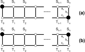
Figure 1: Different source-terminal connections for a simple ladder. Edges and nodes are indexed by their availabilities: $(a_{i},b_{i},c_{i})$ and $(S_{i},T_{i})$.

Using the notation ${\mathcal{R}}_{S_{n}}$ (resp. ${\mathcal{R}}_{T_{n}}$) for the two-terminal availability between $S_{0}$ and $S_{n}$ (resp. $T_{n}$), we find that [16, 18]

$${\mathcal{R}}_{S_{n}} = (1\hskip 5.69054pt0\hskip 5.69054pt0)\,M_{n}\,\cdots\,M_{0}\,\left(\begin{array}[]{ccc}1\\ 0\\ 0\end{array}\right)\,,$$ (22)

$${\mathcal{R}}_{T_{n}} = (0\hskip 5.69054pt1\hskip 5.69054pt0)\,M_{n}\,\cdots\,M_{0}\,\left(\begin{array}[]{ccc}1\\ 0\\ 0\end{array}\right)\,.$$ (26)

The transfer matrix $M_{n}$ is given by

$$M_{n}=\left(\begin{array}[]{lll}a_{n}\,S_{n}&b_{n}\,c_{n}\,S_{n}\,T_{n}&a_{n}\,b_{n}\,c_{n}\,S_{n}\,T_{n}\\ a_{n}\,b_{n}\,S_{n}\,T_{n}&c_{n}\,T_{n}&a_{n}\,b_{n}\,c_{n}\,S_{n}\,T_{n}\\ -a_{n}\,b_{n}\,S_{n}\,T_{n}&-b_{n}\,c_{n}\,S_{n}\,T_{n}&a_{n}\,(1-2\,b_{n})\,c_{n}\,S_{n}\,T_{n}\end{array}\right)\,.$$ (27)

For $n=0$, we must set $a_{0}=1$, and may choose $c_{0}=0$ because it does not change the final result. It is worth noting that all five availabilities of the $n^{\rm th}$ “cell” or building block of the network appear in a single transfer matrix $M_{n}$, which is not sparse, contrary to the matrices of Section III.

Equations (22–27) apply to the most general ladder in terms of individual availabilities. If an edge or a node is missing, its reliability $p_{i}$ should be set to zero, and its failure rate may be considered arbitrary, because it will not alter the final result. Similarly, if a given edge or node is perfect, its reliability should be equal to one; its failure rate $\lambda_{i}$ should then, of course, be set to zero.

The associated matrix $M^{\prime}_{n}$ is

$$M^{\prime}_{n}=\left(\begin{array}[]{lll}m^{\prime}_{11}&m^{\prime}_{12}&m^{\prime}_{13}\\ m^{\prime}_{21}&m^{\prime}_{22}&m^{\prime}_{23}\\ m^{\prime}_{31}&m^{\prime}_{32}&m^{\prime}_{33}\end{array}\right)\,,$$ (28)

with

$$m^{\prime}_{11} = (\lambda_{a_{n}}+\lambda_{S_{n}})\,a_{n}\,S_{n}\,,$$

$$m^{\prime}_{12} = (\lambda_{b_{n}}+\lambda_{c_{n}}+\lambda_{S_{n}}+\lambda_{T_{n}})\,b_{n}\,c_{n}\,S_{n}\,T_{n}\,,$$

$$m^{\prime}_{13} = (\lambda_{a_{n}}+\lambda_{b_{n}}+\lambda_{c_{n}}+\lambda_{S_{n}}+\lambda_{T_{n}})\,a_{n}\,b_{n}\,c_{n}\,S_{n}\,T_{n}\,,$$

$$m^{\prime}_{21} = (\lambda_{a_{n}}+\lambda_{b_{n}}+\lambda_{S_{n}}+\lambda_{T_{n}})\,a_{n}\,b_{n}\,S_{n}\,T_{n}\,,$$

$$m^{\prime}_{22} = (\lambda_{c_{n}}+\lambda_{T_{n}})\,c_{n}\,T_{n}\,,$$

$$m^{\prime}_{23} = m^{\prime}_{13}\,,$$

$$m^{\prime}_{31} = -m^{\prime}_{21}\,,$$

$$m^{\prime}_{32} = -m^{\prime}_{12}\,,$$

$$m^{\prime}_{33} = (\lambda_{a_{n}}+\lambda_{c_{n}}+\lambda_{S_{n}}+\lambda_{T_{n}})\,a_{n}\,c_{n}\,S_{n}\,T_{n}-2\,m^{\prime}_{13}\,.$$

When $a_{i}=b_{i}=c_{i}\equiv p$ and $S_{i}=T_{i}\equiv\rho$ the three eigenvalues $\zeta_{0}$ and $\zeta_{\pm}$ of the transfer matrix are [16]

$$\zeta_{0} = p\,\rho\,(1-p\,\rho),$$ (29)

$$\zeta_{\pm} = \frac{p\,\rho}{2}\,\left(1+2\,p\,(1-p)\,\rho\pm\sqrt{{\mathcal{B}}}\right)\,,$$ (30)

with ${\mathcal{B}}=1+4\,p^{2}\,\rho-8\,p^{3}\,\rho^{2}+4\,p^{4}\,\rho^{2}$. The two-terminal availabilities are [16]

$${\mathcal{R}}_{T_{n}}(p,\rho) = \frac{1}{2\,p}\,\left(-\zeta_{0}^{n+1}+p\,\rho\,(1+p\,\rho)\,\frac{\zeta_{+}^{n+1}-\zeta_{-}^{n+1}}{\zeta_{+}-\zeta_{-}}\right.$$ (31)

$$\left.-(1-2\,p+p\,\rho)\,p^{3}\,\rho^{3}\,\frac{\zeta_{+}^{n}-\zeta_{-}^{n}}{\zeta_{+}-\zeta_{-}}\right)\,,$$

$${\mathcal{R}}_{S_{n}}(p,\rho) = \frac{1}{2\,p}\,\left(+\zeta_{0}^{n+1}+p\,\rho\,(1+p\,\rho)\,\frac{\zeta_{+}^{n+1}-\zeta_{-}^{n+1}}{\zeta_{+}-\zeta_{-}}\right.$$ (32)

$$\left.-(1-2\,p+p\,\rho)\,p^{3}\,\rho^{3}\,\frac{\zeta_{+}^{n}-\zeta_{-}^{n}}{\zeta_{+}-\zeta_{-}}\right)\,.$$

These expressions are identical except for the $\pm$ sign in front of the $\zeta_{0}^{n+1}$ term. Assuming that the common link failure rate is $\lambda$ while that for the nodes is $\xi$, the failure frequency for the $S_{0}\rightarrow T_{n}$ connection is

$$\overline{\nu}=\lambda\,p\,\frac{\partial{\mathcal{R}}_{T_{n}}(p,\rho)}{\partial p}+\xi\,\rho\,\frac{\partial{\mathcal{R}}_{T_{n}}(p,\rho)}{\partial\rho}\,;$$ (33)

a similar expression applies to ${\mathcal{R}}_{S_{n}}(p,\rho)$. When $n$ is large, both availabilities are actually of the form $\alpha_{+}\,\zeta_{+}^{n}$, because the modulus of $\zeta_{+}$ is larger than that of the remaining eigenvalues for $0\leq p\leq 1$ [16]. When nodes are perfect, we have therefore in this limit

$$\overline{\nu}\approx\lambda\,p\,\left(\frac{\partial\alpha_{+}}{\partial p}\,\zeta_{+}^{n}+n\,\alpha_{+}\,\frac{\partial\zeta_{+}}{\partial p}\,\zeta_{+}^{n-1}\right)\,,$$ (34)

so that the failure rate is

$$\overline{\lambda}\approx\lambda\,\left(\frac{\partial\ln\alpha_{+}}{\partial\ln p}+n\,\frac{\partial\ln\zeta_{+}}{\partial\ln p}\right)\,,$$ (35)

with

$$\frac{\partial\ln\zeta_{+}}{\partial\ln p} = \frac{-1+4\,p-6\,p^{2}+4\,p^{3}+(3-4\,p)\,\sqrt{1+4\,p^{2}\,(1-p)^{2}}}{2\,(1-p)\,\sqrt{1+4\,p^{2}\,(1-p)^{2}}}\,,$$ (36)

$$\frac{\partial\ln\alpha_{+}}{\partial\ln p} = \frac{4-5\,p+8\,p^{2}-20\,p^{3}+16\,p^{4}-4\,p^{5}-(4-7\,p+4\,p^{2}-2\,p^{3})\,\sqrt{1+4\,p^{2}\,(1-p)^{2}}}{2\,(1-p)\,[1+4\,p^{2}\,(1-p)^{2}]}\,.$$ (37)

The variations with $p$ of $\partial\ln\zeta_{+}/\partial\ln p$ and $\partial\ln\alpha_{+}/\partial\ln p$ are displayed in Figs. 2 and 3. Since $|\zeta_{+}|<1$ for $p<1$, the contribution of $\partial\ln\alpha_{+}/\partial\ln p$ will prevail, and $\overline{\lambda}$ will have a linear dependence with $n$ in the large network limit (this is a general property when the eigenvalue of highest modulus is different from unity).

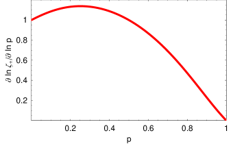
Figure 2: Variation of $\partial\ln\zeta_{+}/\partial\ln p$ with $p$ for a simple ladder with perfect nodes (eq. (36)). The maximum, reached for $p\approx 0.251641$, is about $1.13827$.

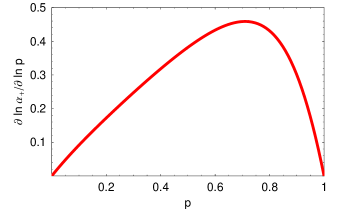
Figure 3: Variation of $\partial\ln\alpha_{+}/\partial\ln p$ with $p$ for a simple ladder with perfect nodes (eq. (37)). The maximum, reached for $p\approx 0.709902$, is about $0.458825$.

For very reliable components, eqs. (35–37) simplify. It is easy to show by a series expansion in the link unavailability $q$ that the global failure rate is given (to first order) by $\overline{\lambda}\to(2\,n+4)\,\lambda\,q$; this result could also have been obtained by visual inspection and enumeration of the minimal cuts.

V Conclusion and outlook

We have shown that the linear differential method for computing the failure frequency is a very simple and useful one for $k$-out-of-$n$ systems as well as the two-terminal availability for recursive networks (this should hold for the all-terminal availability, too [18]). Its application is not limited to the case of extremely reliable components. Even though we restricted our discussion to expressions dealing with availabilities, a similar treatment could be performed for expressions where unavailabilities are the input data (see eq. (2)). For more complex networks, the size of the transfer matrix increases (for instance, it is a $13\times 13$ one for the ‘street $3\times n$’ of [26]) but the calculations remain straightforward. Finally, the expressions given for steady-state availabilities can also be used for time-dependent systems provided that failures and reparations are still statistically independent events, because the expressions are formally identical (the availabilities of components must be replaced by the reliabilities).

Appendix A Proof of eq. (13)

$A_{k,n}$ is given by

$$A_{k,n}=\sum_{l=k}^{n}\,\left(\!\!\!\begin{array}[]{c}n\\ l\end{array}\!\!\!\right)\,p^{l}\,(1-p)^{n-l}\,.$$ (38)

The fundamental equality between binomials

$$\left(\!\!\!\begin{array}[]{c}n+1\\ l\end{array}\!\!\!\right)=\left(\!\!\!\begin{array}[]{c}n\\ l\end{array}\!\!\!\right)+\left(\!\!\!\begin{array}[]{c}n\\ l-1\end{array}\!\!\!\right)\,$$ (39)

leads to

$$A_{k,n+1}=(1-p)\,A_{k,n}+p\,A_{k-1,n}\,.$$ (40)

Setting $\displaystyle{\mathcal{G}}_{k}(z)=\sum_{n=0}^{\infty}\,A_{k,n}\,z^{n}$ implies

$$\frac{1}{z}\,{\mathcal{G}}_{k}(z)=(1-p)\,{\mathcal{G}}_{k}(z)+p\,{\mathcal{G}}_{k-1}(z)\,.$$ (41)

so that

$${\mathcal{G}}_{k}(z)=\frac{p\,z}{1-(1-p)\,z}\,{\mathcal{G}}_{k-1}(z)=\left(\frac{p\,z}{1-(1-p)\,z}\right)^{k}\,{\mathcal{G}}_{0}(z)\,.$$ (42)

Since $A_{0,n}=1,\forall n$, ${\mathcal{G}}_{0}(z)=1/(1-z)$; eq. (13) follows.

Annie Druault-Vicard joined France Telecom Division R&D in 2000. She obtained a PhD in computer science from Institut National de Recherche en Informatique et Automatique (INRIA-Rocquencourt) in 1999.

Christian Tanguy joined the Centre National d’Études des Télécommunications in 1987, and worked in the Laboratoire de Bagneux from 1990 until 2001. He obtained a PhD in atomic physics from University Paris 6 in 1983 and a “Habilitation à diriger des recherches” in condensed matter physics from University Paris 7 in 1996.

References

- [1] M. L. Shooman, Probabilistic reliability: an engineering approach, McGraw-Hill, New York, 1968.
- [2] C. Singh and R. Billinton, System reliability modelling and evaluation, Hutchinson, London, 1977.
- [3] C. J. Colbourn, The Combinatorics of Network Reliability, Oxford University Press, Oxford, 1987.
- [4] W. Kuo and M. J. Zuo, Optimal Reliability Modeling: Principles and Applications, Wiley, Hoboken, 2003.
- [5] C. Singh and R. Billinton, “A new method to determine the failure frequency of a complex system,” IEEE Trans. Reliability, vol. R-23, pp. 231–234, October 1974.
- [6] C. Singh, “Tie set approach to determine the frequency of system failure,” Microelectron. & Reliab., vol. 14, pp. 293–294, 1975.
- [7] W. G. Schneeweiss, “Computing failure frequency, MTBF & MTTR via mixed products of availabilities and unavailabilities,” IEEE Trans. Reliability, vol. R-30, pp. 362–363, October 1981.
- [8] D.-H. Shi, “General formulas for calculating the steady-state frequency of system failure,” IEEE Trans. Reliability, vol. R-30, pp. 444–447, December 1981.
- [9] J. Yuan and S.-B. Chou, “Boolean algebra method to calculate network system reliability indices in terms of a proposed FMEA,” Reliability Engineering, vol. 14, pp. 193–203, 1986.
- [10] S. V. Amari, “Generic rules to evaluate system-failure frequency,” IEEE Trans. Reliability, vol. 49, pp. 85–87, March 2000.
- [11] W. G. Schneeweiss, “Addendum to: Computing failure frequency via mixed products of availabilities and unavailabilities,” IEEE Trans. Reliability, vol. R-32, pp. 461–462, December 1983.
- [12] M. Hayashi, “System failure-frequency analysis using a differential operator,” IEEE Trans. Reliability, vol. 40, pp. 601–609, 614, December 1991.
- [13] J. P. Gadani, “System effectiveness evaluation using star and delta transformations,” IEEE Transactions on Reliability, vol. 30, pp. 43–47, April 1981.
- [14] Y.-R. Chang, S. V. Amari, and S.-Y. Kuo, “Computing System Failure Frequencies and Reliability Importance Measures Using OBDD,” IEEE Trans. Computers, vol. 53, pp. 54–68, January 2004.
- [15] M. Hayashi, T. Abe, and I. Nakajima, “Transformation from availability expression to failure frequency expression,” IEEE Trans. Reliability, vol. 55, pp. 252–261, June 2006.
- [16] C. Tanguy, “Exact solutions for the two- and all-terminal reliabilities of a simple ladder network,” submitted to Networks.
- [17] C. Tanguy, “Exact solutions for the two- and all-terminal reliabilities of the Brecht-Colbourn ladder and the generalized fan,” submitted to Discrete Applied Mathematics.
- [18] C. Tanguy, “What is the probability of connecting two points ?,” submitted to Europhysics Letters.
- [19] M. T. Chao, J. C. Fu, and M. V. Koutras, “Survey of reliability studies of consecutive--out-of-:F & related systems,” IEEE Trans. Reliability, vol. 44, pp. 120–127, March 1995.
- [20] W. Kuo, J. C. Fu, and F. K. Hwang, “Opinions on consecutive--out-of-:F systems,” IEEE Trans. Reliability, vol. 43, pp. 659–662, December 1994.
- [21] E. R. Canfield and W. P. McCormick, “Asymptotic reliability of consecutive k-out-of-n systems,” J. of Appl. Prob., vol. 29, pp. 142–155, March 1992.
- [22] This expression shows that for ( is an obvious zero of the denominator of ) a partial fraction decomposition of eq. (18) gives the explicit, analytical and slightly tedious expression of the eigenvalues as functions of .
- [23] K. D. Heidtmann, “Smaller sums of disjoint products by subproduct inversion,” IEEE Trans. Reliability, vol. 38, pp. 305–311, 1989.
- [24] A. Rauzy, “A new methodology to handle Boolean models with loops,” IEEE Trans. Reliability, vol. 52, pp. 96–105, 2003.
- [25] S. Kuo, S. Lu, and F. Yeh, “Determining terminal pair reliability based on edge expansion diagrams using OBDD,” IEEE Trans. Reliability, vol. 48 (3) (1999), 234–246.
- [26] F. M. Yeh, S. K. Lu, and S. Y. Kuo, “OBDD-based evaluation of k-terminal network reliability,” IEEE Trans. Reliability, vol. 51, pp. 443–451, 2002.
- [27] Fu-Min Yeh, Hung-Yau Lin, and Sy-Yen Kuo, “Analyzing network reliability with imperfect nodes using OBDD,” Proceedings of the 2002 Pacific Rim International Symposium on Dependable Computing (PRDC’02), pp. 89–96.
- [28] D. R. Shier, Network Reliability and Algebraic Structures, Clarendon Press, Oxford, 1991.