The Effect of Finite Rate Feedback on CDMA Signature Optimization and MIMO Beamforming Vector Selection^∗

Abstract

We analyze the effect of finite rate feedback on CDMA (code-division multiple access) signature optimization and MIMO (multi-input-multi-output) beamforming vector selection. In CDMA signature optimization, for a particular user, the receiver selects a signature vector from a codebook to best avoid interference from other users, and then feeds the corresponding index back to the specified user. For MIMO beamforming vector selection, the receiver chooses a beamforming vector from a given codebook to maximize throughput, and feeds back the corresponding index to the transmitter. These two problems are dual: both can be modeled as selecting a unit norm vector from a finite size codebook to “match” a randomly generated Gaussian matrix. In signature optimization, the least match is required while the maximum match is preferred for beamforming selection.

Assuming that the feedback link is rate limited, our main result is an exact asymptotic performance formula where the length of the signature/beamforming vector, the dimensions of interference/channel matrix, and the feedback rate approach infinity with constant ratios. The proof rests on a large deviation principle over a random matrix ensemble. Further, we show that random codebooks generated from the isotropic distribution are asymptotically optimal not only on average, but also with probability one.

I Introduction

In a direct-sequence code-division multiple access (DS-CDMA) system, the performance is mainly limited by interference among users. We assume that the receiver (base station) has perfect information of all users’ signature. For a particular user, the receiver selects a signature to minimize the interference from other users, and then feeds the corresponding index to the specified user through a feedback link. Dually, consider a multi-input-multi-output (MIMO) system with beamforming vector selection. Take the Rayleigh fading channel model, where the channel matrix has independent and identically distributed (i.i.d.) symmetric complex Gaussian entries with mean zero and unit variance ($\mathcal{CN}\left(0,1\right)$). Now assume that the receiver knows the channel state matrix perfectly. To aid the transmitter, the receiver chooses a beamforming vector from the codebook to maximize the throughput, and then feeds back the corresponding index to the transmitter. In both scenarios, we consider a finite feedback rate up to $R_{\mathrm{fb}}$ bits. Ideally, if the feedback rate is unlimited, the transmitter is able to obtain interference/channel information with arbitrary accuracy, but this is not practically feasible and it is essential to real systems to understand the effect of finite rate feedback.

This paper is the first to rigorously obtain exact asymptotic performance formulae for both problems when letting the length of the signature/beamforming vector, the dimensions of interference/channel matrix, and the feedback rate approach infinity with constant ratios. The same set-ups had been considered previously in [1] and [2], in which a one-sided bound was presented (this was a lower bound on the CDMA performance, and an upper bound in the case of MIMO). Our approach is fundamentally different. Identifying the underlying problem as a large deviation question for the connected random matrix ensemble, we have a unified framework which handles both CDMA and MIMO cases simultaneously. Further, while [2] discusses the fact that random codebooks are asymptotically optimal on average (their mean performance is the best achievable performance), here we prove the stronger result that random codebooks are asymptotically optimal with probability one.

The paper is organized as follows. After describing the system models in more detail, Section III presents various needed facts from Random Matrix Theory. Section IV contains the main results. The basic convergence result is Theorem 1, which in turn is based on a random codebook version, Theorem 2, along with a separate argument that any given codebook will not asymptotically outperform its random counterpart. This section concludes with the almost sure optimality, Theorem 4. Once again, all this is based on a large deviation principle for the spectrum of a Wishart type random matrix. That proof is found in the appendices.

Remark 1

Our methods carry over to the problem of the average throughput of an MMSE receiver in CDMA systems. Each appearance of $\frac{1}{n}\mathbf{H}\mathbf{H}^{\dagger}$, in say (2) below, is replaced by $\left(\mathbf{I}+\frac{1}{n}\mathbf{H}\mathbf{H}^{\dagger}\right)^{-1}$, and the proof may be followed verbatim except for the few obvious (and trivial) modifications.

II System Model

II-A CDMA Signature Optimization

In a sampled discrete-time symbol-synchronous DS-CDMA system with $m$ users, the received vector $\mathbf{Y}$ can be written as

$$\mathbf{Y}=\sum_{j=1}^{m}B_{j}\mathbf{s}_{j}+\mathbf{W},$$

where $B_{j}\in\mathbb{C}$ and $\mathbf{s}_{j}\in\mathbb{C}^{n\times 1}$ are the transmitted symbol and the signature vector for user $j$ respectively, and $\mathbf{W}\in\mathbb{C}^{n\times 1}$ is the additive white Gaussian noise vector with zero mean and covariance matrix $\sigma^{2}\mathbf{I}$. Throughout this paper, we assume that the transmitted symbols $B_{j}$’s are i.i.d. $\mathcal{CN}\left(0,1\right)$ random variables. The signature vectors $\mathbf{s}_{j}$’s satisfy $\mathbf{s}_{j}^{\dagger}\mathbf{s}_{j}=1$, $1\leq j\leq m$. Their length $n$ is often referred to as processing gain in literature.

This paper focuses on matched filter receiver. As already mentioned, the analysis for a MMSE receiver is effectively the same. With a matched filter receiver, the throughput of user $1$ is

$$\log\left(1+\frac{1}{\sigma^{2}+\sum_{j=2}^{m}\mathbf{s}_{1}^{\dagger}\mathbf{S}_{1}\mathbf{S}_{1}^{\dagger}\mathbf{s}_{1}}\right),$$

where $\mathbf{S}_{1}=\left[\mathbf{s}_{2}\cdots\mathbf{s}_{m}\right]$.

The signature optimization is described as follows. Assume that the receiver has perfect knowledge of the $\mathbf{s}_{j}$’s. It guides a particular user, say user 1, to avoid the others’ interference. Here, a codebook $\mathcal{B}$ of signature vectors is declared to both the receiver and user 1. Given the other users’ signatures $\mathbf{s}_{2},\cdots,\mathbf{s}_{m}$, the receiver selects

$$\mathbf{s}_{1}=\underset{\mathbf{v}\in\mathcal{B}}{\arg\;\min}\;\mathbf{v}^{\dagger}\mathbf{S}_{1}\mathbf{S}_{1}^{\dagger}\mathbf{v}.$$

Then it feeds the corresponding index back to user $1$ through a finite rate feedback link, whose rate is up to $R_{\mathrm{fb}}$ bits. This finite feedback rate assumption imposes a constraint on the size of the codebook, $\left|\mathcal{B}\right|\leq 2^{R_{\mathrm{fb}}}$. Therefore, the average interference for user $1$ is given by

$$\underset{\mathcal{B}:\;\left|\mathcal{B}\right|\leq 2^{R_{\mathrm{fb}}}}{\inf}\mathrm{E}_{\mathbf{S}_{1}}\left[\underset{\mathbf{v}\in\mathcal{B}}{\min}\;\mathbf{v}^{\dagger}\mathbf{S}_{1}\mathbf{S}_{1}^{\dagger}\mathbf{v}\right].$$

II-B MIMO Beamforming Vector Selection

The signal model for a MIMO system with beamforming vector selection is

$$\mathbf{Y}=\mathbf{H}^{\dagger}\mathbf{q}X+\mathbf{W},$$

where $\mathbf{Y}\in\mathbb{C}^{m\times 1}$ is the received signal vector, $\mathbf{H}\in\mathbb{C}^{n\times m}$ is the channel state matrix, $\mathbf{q}\in\mathbb{C}^{n\times 1}$ is the beamforming vector satisfying $\mathbf{q}^{\dagger}\mathbf{q}=1$, $X$ is the transmitted signal $\mathcal{CN}\left(0,1\right)$, $\mathbf{W}\in\mathbb{C}^{m\times 1}$ is the white Gaussian noise vector with mean zero and covariance $\sigma^{2}\mathbf{I}_{m}$. The dimensions $n$ and $m$ are the numbers of antennas at the transmitter and receiver.

In the above setting, beamforming vector selection proceeds as follows. Assume that the receiver knows the realization of $\mathbf{H}$ perfectly, and feeds beamforming vector selection information back to the transmitter through a feedback link with rate up to $R_{\mathrm{fb}}$bits. A codebook $\mathcal{B}$ containing $2^{R_{\mathrm{fb}}}$ many candidate beamforming vector is declared to both transmitter and receiver. For any $\mathbf{H}$ realization, the receiver selects the beamforming vector to maximize the throughput

$$\mathbf{q} =\underset{\mathbf{v}\in\mathcal{B}}{\arg\;\max}\;\log\left|\mathbf{I}_{m}+\frac{1}{\sigma^{2}}\mathbf{H}^{\dagger}\mathbf{v}\mathbf{v}^{\dagger}\mathbf{H}\right|$$

$$=\underset{\mathbf{v}\in\mathcal{B}}{\arg\;\max}\;\mathbf{v}^{\dagger}\left(\frac{1}{n}\mathbf{H}\mathbf{H}^{\dagger}\right)\mathbf{v}.$$

The corresponding index is fed back to the transmitter, which then employs $\mathbf{q}$ for transmission. The average received signal power is

$$\underset{\mathcal{B}:\;\left|\mathcal{B}\right|\leq 2^{R_{\mathrm{fb}}}}{\sup}\mathrm{E}_{\mathbf{H}}\left[\underset{\mathbf{v}\in\mathcal{B}}{\max}\;\mathbf{v}^{\dagger}\left(\frac{1}{n}\mathbf{H}\mathbf{H}^{\dagger}\right)\mathbf{v}\right].$$

II-C Unified Formulation

It is difficult to quantify both the average interference in Section II-A and the average received power in Section II-B. However, when $n$, $m$ and $R_{\mathrm{f}b}$ approach infinity linearly with constant ratios, each converges to a constant. To be precise, let $\mathcal{B}\triangleq\left\{\mathbf{v}\in\mathbb{C}^{n\times 1}:\;\mathbf{v}^{\dagger}\mathbf{v}=1\right\}$ be a codebook. Let $\mathbf{H}\in\mathbb{C}^{n\times m}$ be a random Gaussian matrix with i.i.d. $\mathcal{CN}\left(0,1\right)$ entries. Define

$$c_{\min,n}=\underset{\mathcal{B}:\;\left|\mathcal{B}\right|=2^{R_{\mathrm{fb}}}}{\inf}\mathrm{E}_{\mathbf{H}}\left[\underset{\mathbf{v}\in\mathcal{B}}{\min}\;\mathbf{v}^{\dagger}\left(\frac{1}{n}\mathbf{H}\mathbf{H}^{\dagger}\right)\mathbf{v}\right]$$ (1)

and

$$c_{\max,n}=\underset{\mathcal{B}:\;\left|\mathcal{B}\right|=2^{R_{\mathrm{fb}}}}{\sup}\mathrm{E}_{\mathbf{H}}\left[\underset{\mathbf{v}\in\mathcal{B}}{\max}\;\mathbf{v}^{\dagger}\left(\frac{1}{n}\mathbf{H}\mathbf{H}^{\dagger}\right)\mathbf{v}\right].$$ (2)

As $n,m,R_{\mathrm{fb}}\rightarrow\infty$ with with $\frac{m}{n}\rightarrow\frac{1}{\beta}\in\mathbb{R}^{+}$ and $\frac{R_{\mathrm{fb}}}{n}\rightarrow r\in\mathbb{R}^{+}$, we shall show that $c_{\min,n}$ and $c_{\max,n}$ converge to constants and compute their limits in Section IV.

Remark 2

We assume that $\mathbf{H}\in\mathbb{C}^{n\times m}$ has i.i.d. entries in this unified formulation while the matrix $\mathbf{S}_{1}\in\mathbb{C}^{n\times\left(m-1\right)}$ in the CDMA signature optimization is composed of independent and isotropically distributed columns. Notably, the asymptotic statistics of $\mathbf{S}_{1}\mathbf{S}_{1}^{\dagger}$ and $\frac{1}{n}\mathbf{H}\mathbf{H}^{\dagger}$ are the same as $\frac{m}{n}\rightarrow\frac{1}{\beta}\in\mathbb{R}$. The limit of $c_{\min,n}$ will gives the asymptotic average interference for user 1 in a CDMA system.

III Preliminaries

III-A Asymptotic Random Matrix Theory

The performance calculation is based on the asymptotic spectral distribution of the matrix $\frac{1}{m}\mathbf{H}\mathbf{H}^{\dagger}$. Let $\lambda_{1},\cdots,\lambda_{n}$ be the $n$ singular values of $\frac{1}{m}\mathbf{H}\mathbf{H}^{\dagger}$. Define the empirical distribution of the singular values

$$\mu_{n,\bm{\lambda}}\left(\lambda\right)\triangleq\frac{1}{n}\left|\left\{j:\;\lambda_{j}\leq\lambda\right\}\right|.$$

As $n,m\rightarrow\infty$ with $\frac{m}{n}\rightarrow\frac{1}{\beta}\in\mathbb{R}^{+}$,

$$d\mu_{\lambda}=\underset{\left(n,m\right)\rightarrow\infty}{\lim}d\mu_{n,\bm{\lambda}}\left(\lambda\right)=\left(\left(1-\frac{1}{\beta}\right)^{+}\delta\left(\lambda\right)+\frac{\sqrt{\left(\lambda-\lambda^{-}\right)^{+}\left(\lambda^{+}-\lambda\right)^{+}}}{2\pi\beta\lambda}\right)\,d\lambda$$ (3)

almost surely, where $\lambda^{\pm}=\left(1\pm\sqrt{\beta}\right)^{2}$ and $\left(x\right)^{+}=\max\left(x,0\right)$. (A good reference for this type of result is [5].) For later it will be useful to define

$$\lambda_{t}^{-}\triangleq\begin{cases}0&\mathrm{if}\;\beta\geq 1\\ \lambda^{-}&\mathrm{if}\;\beta<1\end{cases},\;\mathrm{and}\;\bar{\lambda}=\int\lambda\cdot d\mu_{\lambda}.$$

Consider as well a linear spectral statistic

$$g\left(\frac{1}{m}\mathbf{H}\mathbf{H}^{\dagger}\right)=\frac{1}{n}\sum_{i=1}^{n}g\left(\lambda_{i}\right).$$

If $g$ is Lipschitz on $\left[\lambda_{t}^{-},\lambda^{+}\right]$, then we also have that

$$\underset{\left(n,m\right)\rightarrow\infty}{\lim}g\left(\frac{1}{m}\mathbf{H}\mathbf{H}^{\dagger}\right)=\int g\left(\lambda\right)d\mu_{\lambda}$$

almost surely, see for example [6] for a modern approach.

Last, the asymptotic properties of the minimum and maximum eigenvalues will figure into our analysis. For any finite $n$, set $\lambda_{\min,\bm{\lambda}}=\underset{1\leq i\leq n}{\min}\lambda_{i}$ and $\lambda_{\max,\bm{\lambda}}=\underset{1\leq i\leq n}{\max}\lambda_{i}$.

Proposition 1

Let $n,m\rightarrow\infty$ linearly with $\frac{m}{n}\rightarrow\frac{1}{\beta}\in\mathbb{R}^{+}$.

1. $\lambda_{\min,n}\rightarrow\lambda_{t}^{-}$ and $\lambda_{\max,n}\rightarrow\lambda^{+}$ almost surely.

2. All moments of $\lambda_{\min,n}$ and $\lambda_{\max,n}$ also converge.

The almost sure convergence goes back to [7, 8]. The convergence of moments is implied by the results in [9]. A direct application of this proposition is that for $\forall A_{n}\subset\mathbb{R}^{n}$ such that $\mu_{n,\bm{\lambda}}\left(A_{n}\right)\rightarrow 0$, $\mathrm{E}_{\bm{\lambda}}\left[\lambda_{\max,\bm{\lambda}},\;A_{n}\right]\rightarrow 0$; this fact will be employed repeatedly below.

III-B Isotropic Distribution

We also bring in the isotropic distribution for

$$\mathcal{U}_{n\times m}\triangleq\left\{\mathbf{U}\in\mathbb{C}^{n\times m}:\;\mathbf{U}^{\dagger}\mathbf{U}=\mathbf{I}_{m}\right\},$$

by which we mean the (left) Haar measure $\mu$ of $\mathcal{U}_{n\times m}$. In particular, for any set $\mathcal{M}\subset\mathcal{U}_{n\times m}$ and any $\mathbf{U}\in\mathcal{U}_{n\times n}$, $\mu\left(\mathbf{U}\mathcal{M}\right)=\mu\left(\mathcal{M}\right)$.

IV Main Results

For $\forall x\in\left(\lambda_{t}^{-},\lambda^{+}\right)$, define

$$\psi_{x}\left(\alpha\right) \triangleq\begin{cases}-\int\log\left(1-\alpha\left(\lambda-x\right)\right)d\mu_{\lambda}&\mathrm{if}\;\alpha\in\left[-\frac{1}{x-\lambda_{t}^{-}},\frac{1}{\lambda^{+}-x}\right]\\ +\infty&\mathrm{otherwise}\end{cases}$$ (4)

and

$$\psi_{x}^{*}\left(t\right)\triangleq\underset{\alpha\in\mathbb{R}}{\sup}\;\alpha t-\psi_{x}\left(\alpha\right)$$ (5)

for any $t\in\mathbb{R}$. Our basic convergence result for $c_{\min,n}$ and $c_{\max,n}$ reads:

Theorem 1

Let $n$, $m$ and $R_{\mathrm{fb}}$ approach infinity linearly with $\frac{m}{n}\rightarrow\frac{1}{\beta}\in\mathbb{R}^{+}$ and $\frac{R_{\mathrm{fb}}}{n}\rightarrow r\in\mathbb{R}^{+}$. There exist unique $x_{r}^{-}\in\left(\lambda_{t}^{-},\bar{\lambda}\right)$ and $x_{r}^{+}\in\left(\bar{\lambda},\lambda^{+}\right)$ such that $r\log 2=\psi_{x_{r}^{-}}^{*}\left(0\right)=\psi_{x_{r}^{+}}^{*}\left(0\right)$. Furthermore,

$$\underset{\left(n,m,R_{\mathrm{fb}}\right)\rightarrow\infty}{\lim}\;c_{\min,n}=x_{r}^{-}/\beta,$$

and

$$\underset{\left(n,m,R_{\mathrm{fb}}\right)\rightarrow\infty}{\lim}\;c_{\max,n}=x_{r}^{+}/\beta.$$

Remark 3

From the properties of $\psi_{x}^{*}\left(0\right)$ (Proposition 4),

$$\begin{cases}c_{\min,n}\rightarrow\bar{\lambda}/\beta,\;c_{\max,n}\rightarrow\bar{\lambda}/\beta&\mathrm{as}\;r\downarrow 0\\ c_{\min,n}\rightarrow\lambda_{t}^{-}/\beta,\;c_{\max,n}\rightarrow\lambda^{+}/\beta\;&\mathrm{as}\;r\uparrow\infty\end{cases}.$$

This is consistent with intuition: $r=0$ and $r=\infty$ representing either no, or perfect information.

Using ideas from [10], we may also obtain fairly explicit formulas for $x_{r}^{-}$ and $x_{r}^{+}$. (It should be noted that [4] also takes on this computation, but from a different vantage point.)

Corollary 1

Let $r_{\min}=\frac{-\log\left(1-\sqrt{\beta}\right)-\sqrt{\beta}}{\beta\log 2}$ for $\forall\beta<1$ and $r_{\max}=\frac{\sqrt{\beta}-\log\left(1+\sqrt{\beta}\right)}{\beta\log 2}$ for $\forall\beta\in\mathbb{R}^{+}$. Then for any $r\in\mathbb{R}^{+}$, $x_{r}^{-}\in\left(\lambda_{t}^{-},1\right)$ satisfies

$$\begin{cases}x_{r}^{-}=\left(1-\sqrt{\beta}\right)^{2}+\sqrt{\beta}\left(1-\sqrt{\beta}\right)^{1-\frac{1}{\beta}}\exp\left(-\frac{1}{\sqrt{\beta}}-r\log 2\right)&\mathrm{if}\;\beta<1\;\mathrm{and}\;r>r_{\min}\\ x_{r}^{-}=e^{x_{r}^{-}-1}2^{-\beta r}&\mathrm{otherwise}\end{cases},$$

and $x_{r}^{+}\in\left(1,\lambda^{+}\right)$ satisfies

$$\begin{cases}x_{r}^{+}=\left(1+\sqrt{\beta}\right)^{2}-\sqrt{\beta}\left(1+\sqrt{\beta}\right)^{1-\frac{1}{\beta}}\exp\left(\frac{1}{\sqrt{\beta}}-r\log 2\right)&\mathrm{if}\;r>r_{\max}\\ x_{r}^{+}=e^{x_{r}^{+}-1}2^{-\beta r}&\mathrm{otherwise}\end{cases}.$$

Granted the existence and uniqueness of $x_{r}^{-}$ and $x_{r}^{+}$, which follow from basic properties of $\psi_{x}^{*}\left(0\right)$ established in Proposition 4 of Appendix -A, the proof of Theorem 1 takes the following course. First, by calculating the average performance of random codes, we are construct upper and lower bounds on $\lim c_{\min,n}$ and $\lim c_{\max,n}$ respectively. Let $\mathcal{B}_{\mathrm{rand}}$ be a randomly constructed codebook of i.i.d. unit-norm vectors from the isotropic distribution. In particular, $\mathcal{B}_{\mathrm{rand}}=\left\{\mathbf{v}_{1},\cdots,\mathbf{v}_{2^{R_{\mathrm{fb}}}}\right\}$, where $\mathbf{v}_{k}=\mathbf{z}_{k}/\left\|\mathbf{z}_{k}\right\|$, $\mathbf{z}_{k}=\left[z_{k,1},\cdots,z_{k,n}\right]^{\dagger}$ and $z_{k,i}$ are i.i.d. $\mathcal{CN}\left(0,1\right)$ for all $1\leq k\leq 2^{R_{\mathrm{fb}}}$ and $1\leq i\leq n$. Define

$$c_{\min,n,\mathrm{rand}}=\mathrm{E}_{\mathcal{B}_{\mathrm{rand}}}\left[\mathrm{E}_{\mathbf{H}}\left[\underset{\mathbf{v}\in\mathcal{B}_{\mathrm{rand}}}{\min}\;\mathbf{v}^{\dagger}\left(\frac{1}{n}\mathbf{H}\mathbf{H}^{\dagger}\right)\mathbf{v}\right]\right]$$

and

$$c_{\max,n,\mathrm{rand}}=\mathrm{E}_{\mathcal{B}_{\mathrm{rand}}}\left[\mathrm{E}_{\mathbf{H}}\left[\underset{\mathbf{v}\in\mathcal{B}_{\mathrm{rand}}}{\max}\;\mathbf{v}^{\dagger}\left(\frac{1}{n}\mathbf{H}\mathbf{H}^{\dagger}\right)\mathbf{v}\right]\right].$$

The following theorem calculates the average performance of random codes.

Theorem 2

As $n,m,R_{\mathrm{fb}}\rightarrow\infty$ with $\frac{m}{n}\rightarrow\frac{1}{\beta}\in\mathbb{R}^{+}$ and $\frac{R_{\mathrm{fb}}}{n}\rightarrow r\in\mathbb{R}^{+}$,

$$\underset{\left(n,m,R_{\mathrm{fb}}\right)\rightarrow\infty}{\lim}\;c_{\min,n,\mathrm{rand}}=x_{r}^{-}/\beta$$

and

$$\underset{\left(n,m,R_{\mathrm{fb}}\right)\rightarrow\infty}{\lim}\;c_{\max,n,\mathrm{rand}}=x_{r}^{+}/\beta.$$

Clearly, $\lim\;c_{\min,n}\leq\lim\;c_{\min,n,\mathrm{rand}}$ and $\lim\;c_{\max,n}\geq\lim\;c_{\max,n,\mathrm{rand}}$, and the next step is to obtain a lower bound $\lim\;c_{\min,n}$ and and upper bound $\lim\;c_{\max,n}$. Introduce the singular value decomposition, $\frac{1}{m}\mathbf{H}\mathbf{H}^{\dagger}=\mathbf{U}\mathbf{\Lambda}\mathbf{U}^{\dagger}$ where $\mathbf{U}\in\mathcal{U}_{n\times n}$ and $\mathbf{\Lambda}\in\mathbb{R}^{n\times n}$ is the diagonal matrix of eigenvalues $\lambda_{1},\cdots,\lambda_{n}$. It is well known that $\mathbf{U}$ is isotropically distributed and independent with $\mathbf{\Lambda}$. For any codebook $\mathcal{B}=\left\{\mathbf{v}\in\mathcal{U}_{n\times 1}\right\}$, define

$$c_{\min,n,\bm{\lambda},\mathcal{B}}\triangleq\mathrm{E}_{\mathbf{U}}\left[\left.\underset{\mathbf{v}\in\mathcal{B}}{\min}\;\mathbf{v}^{\dagger}\mathbf{U}\mathrm{diag}\left(\bm{\lambda}\right)\mathbf{U}^{\dagger}\mathbf{v}\right|\bm{\lambda}\right]$$ (6)

and

$$c_{\max,n,\bm{\lambda},\mathcal{B}}\triangleq\mathrm{E}_{\mathbf{U}}\left[\left.\underset{\mathbf{v}\in\mathcal{B}}{\max}\;\mathbf{v}^{\dagger}\mathbf{U}\mathrm{diag}\left(\bm{\lambda}\right)\mathbf{U}^{\dagger}\mathbf{v}\right|\bm{\lambda}\right].$$ (7)

As $n,m,R_{\mathrm{fb}}\rightarrow\infty$ linearly with constant ratios $\frac{1}{\beta}$ and $r$, Define

$$c_{\min,\bm{\lambda}}\triangleq\underset{\left(n,m,R_{\mathrm{fb}}\right)\rightarrow\infty}{\lim}\;\underset{\mathcal{B}:\;\left|\mathcal{B}\right|=2^{R_{\mathrm{fb}}}}{\inf}\;c_{\min,n,\bm{\lambda},\mathcal{B}}$$

and

$$c_{\max,\bm{\lambda}}\triangleq\underset{\left(n,m,R_{\mathrm{fb}}\right)\rightarrow\infty}{\lim}\;\underset{\mathcal{B}:\;\left|\mathcal{B}\right|=2^{R_{\mathrm{fb}}}}{\inf}\;c_{\max,n,\bm{\lambda},\mathcal{B}}.$$

It is clear that $c_{\min,\bm{\lambda}}$ and $c_{\max,\bm{\lambda}}$ are random variables depending on $\bm{\lambda}$. The following theorem provides bounds on $c_{\min,\bm{\lambda}}$ and $c_{\max,\bm{\lambda}}$, and therefore bounds on $\lim\;c_{\min,n}$ and $\lim\;c_{\max,n}$.

Theorem 3

As $n,\;m,\;R_{\mathrm{fb}}\rightarrow\infty$ with $\frac{m}{n}\rightarrow\frac{1}{\beta}\in\mathbb{R}^{+}$ and $\frac{R_{\mathrm{fb}}}{n}\rightarrow r\in\mathbb{R}^{+}$,

1. $c_{\min,\bm{\lambda}}\geq x_{r}^{-}$ and $c_{\max,\bm{\lambda}}\leq x_{r}^{+}$ with probability 1 in $\bm{\lambda}$, and

2. $\underset{\left(n,m,R_{\mathrm{fb}}\right)\rightarrow\infty}{\lim}c_{\min,n}\geq x_{r}^{-}/\beta$ and $\underset{\left(n,m,R_{\mathrm{fb}}\right)\rightarrow\infty}{\lim}c_{\max,n}\leq x_{r}^{+}/\beta$.

By combining the above results, Theorem 1 is proved.

Finally, while Theorem 2 implies that random codebooks are asymptotically optimal on average, we actually have the stronger result that they are asymptotically optimal with probability one.

Theorem 4

As $n,\;m,\;R_{\mathrm{fb}}\rightarrow\infty$ with $\frac{m}{n}\rightarrow\frac{1}{\beta}\in\mathbb{R}^{+}$ and $\frac{R_{\mathrm{fb}}}{n}\rightarrow r\in\mathbb{R}^{+}$, for any $\epsilon>0$

$$\underset{\left(n,m,R_{\mathrm{fb}}\right)\rightarrow\infty}{\lim}\mu_{n,\mathcal{B}_{\mathrm{rand}}}\left(\mathrm{E}_{\mathbf{H}}\left[\underset{\mathbf{v}\in\mathcal{B}_{\mathrm{rand}}}{\min}\frac{1}{n}\mathbf{v}^{\dagger}\mathbf{H}\mathbf{H}^{\dagger}\mathbf{v}\right]>\beta\cdot x_{r}^{-}+\epsilon\right)=0$$

and

$$\underset{\left(n,m,R_{\mathrm{fb}}\right)\rightarrow\infty}{\lim}\mu_{n,\mathcal{B}_{\mathrm{rand}}}\left(\mathrm{E}_{\mathbf{H}}\left[\underset{\mathbf{v}\in\mathcal{B}_{\mathrm{rand}}}{\max}\frac{1}{n}\mathbf{v}^{\dagger}\mathbf{H}\mathbf{H}^{\dagger}\mathbf{v}\right]<\beta\cdot x_{r}^{+}-\epsilon\right)=0.$$

Remark 4

The asymptotic achievable throughputs of the above CDMA and MIMO systems are

$$\log\left(1+\frac{1}{\sigma^{2}+\lim\;c_{\min,n}}\right)$$

and

$$\log\left(1+\frac{\lim\;c_{\max,n}}{\sigma^{2}}\right)$$

respectively. These facts are direct applications of the proof of Theorem 3.

The proofs of Theorem 2-4 occupy the next sections (IV-A-IV-C). The key step is a large deviation principle established in Theorem 5 in Appendix -B. Last, the computation in Corollary 1 is conducted in Appendix -C.

IV-A Average Performance of Random Codes

Since the calculations of $c_{\max,n,\mathrm{rand}}$ and $c_{\min,n,\mathrm{rand}}$ follow the same line, we only give the details for $c_{\min,n,\mathrm{rand}}$. In the following, we first prove that

$$\underset{\left(n,m,R_{\mathrm{fb}}\right)\rightarrow\infty}{\lim}\;c_{\min,n,\mathrm{rand}}\geq x_{r}^{-}/\beta$$ (8)

by Chebyshev’s inequality, then show that

$$\underset{\left(n,m,R_{\mathrm{fb}}\right)\rightarrow\infty}{\lim}\;c_{\min,n,\mathrm{rand}}\leq x_{r}^{-}/\beta$$ (9)

by exponential change of a probability measure.

We express $c_{\min,n,\mathrm{rand}}$ in a convenient form. Recall the singular value decomposition $\frac{1}{m}\mathbf{H}\mathbf{H}^{\dagger}=\mathbf{U}\mathbf{\Lambda}\mathbf{U}^{\dagger}$.

$$c_{\min,n,\mathrm{rand}} =\mathrm{E}_{\mathbf{H}}\left[\mathrm{E}_{\mathcal{B}_{\mathrm{rand}}}\left[\frac{1}{n}\underset{k}{\min}\frac{\mathbf{z}_{k}^{\dagger}\mathbf{H}\mathbf{H}^{\dagger}\mathbf{z}_{k}}{\left\|\mathbf{z}_{k}\right\|^{2}}\right]\right]$$

$$=\frac{m}{n}\mathrm{E}_{\mathbf{H}}\left[\mathrm{E}_{\mathcal{B}_{\mathrm{rand}}}\left[\underset{k}{\min}\frac{\mathbf{z}_{k}^{\dagger}\left(\frac{1}{m}\mathbf{H}\mathbf{H}^{\dagger}\right)\mathbf{z}_{k}}{\left\|\mathbf{z}_{k}\right\|^{2}}\right]\right]$$

$$=\frac{m}{n}\mathrm{E}_{\mathbf{H}}\left[\mathrm{E}_{\mathcal{B}_{\mathrm{rand}}}\left[\underset{k}{\min}\frac{\mathbf{z}_{k}^{\dagger}\mathbf{U}\mathbf{\Lambda}\mathbf{U}^{\dagger}\mathbf{z}_{k}}{\left\|\mathbf{z}_{k}\right\|^{2}}\right]\right]$$

$$=\frac{m}{n}\mathrm{E}_{\mathbf{H}}\left[\mathrm{E}_{\mathcal{B}_{\mathrm{rand}}}\left[\underset{k}{\min}\frac{\sum_{i=1}^{n}\lambda_{i}\left|z_{k,i}\right|^{2}}{\sum_{i=1}^{n}\left|z_{k,i}\right|^{2}}\right]\right],$$

where the last equality follows from the fact that $\mathbf{z}_{k}$ and $\mathbf{U}\mathbf{z}_{k}$ are statistically equal for any given $n\times n$ unitary matrix $\mathbf{U}$. Let $Y_{k,i}=\left|Z_{k,i}\right|^{2}$. Then $Y_{k,i}$’s ($1\leq k\leq 2^{R_{\mathrm{fb}}}$ and $1\leq i\leq n$) are i.i.d. random variables with probability measure $d\mu_{y}=e^{-y}dy$. Note that for a given $\bm{\lambda}$ vector, the random variables $\sum_{i=1}^{n}\lambda_{i}Y_{k,i}/\sum_{i=1}^{n}Y_{k,i}$’s ($k=1,\cdots,2^{R_{\mathrm{fb}}}$) are conditional independent (conditioned on $\bm{\lambda}$). Define the corresponding conditional probability measure

$$\mu_{n,\mathbf{Y}}\left(x|\bm{\lambda}\right) \triangleq\mu_{n,\mathbf{Y}}\left(\left.\frac{\sum_{i=1}^{n}\lambda_{i}Y_{i}}{\sum_{i=1}^{n}Y_{i}}\leq x\right|\bm{\lambda}\right)$$ (10)

$$=\mu_{n,\mathbf{Y}}\left(\left.\sum_{i=1}^{n}\left(\lambda_{i}-x\right)Y_{i}\leq 0\right|\bm{\lambda}\right).$$

Then

$$\Pr\left(\left.\underset{k}{\min}\frac{\sum_{i=1}^{n}\lambda_{i}Y_{i}}{\sum_{i=1}^{n}Y_{i}}\leq x\right|\bm{\lambda}\right)=1-\left(1-\mu_{n,\mathbf{Y}}\left(x|\bm{\lambda}\right)\right)^{2^{R_{\mathrm{fb}}}}.$$

Thus

$$\mathrm{E}_{\mathcal{B}_{\mathrm{rand}}}\left[\underset{k}{\min}\frac{\sum_{i=1}^{n}\lambda_{i}\left|z_{k,i}\right|^{2}}{\sum_{i=1}^{n}\lambda_{i}\left|z_{k,i}\right|^{2}}\right]=\lambda_{\min,\bm{\lambda}}+\int_{\lambda_{\min,\bm{\lambda}}}^{\lambda_{\max,\bm{\lambda}}}\left(1-\mu_{n,\mathbf{Y}}\left(x|\bm{\lambda}\right)\right)^{2^{R_{\mathrm{fb}}}}dx$$

and

$$c_{\min,n,\mathrm{rand}}=\frac{\min\left(n,m\right)}{n}\mathrm{E}_{\bm{\lambda}}\left[\lambda_{\min,\bm{\lambda}}+\int_{\lambda_{\min,\bm{\lambda}}}^{\lambda_{\max,\bm{\lambda}}}\left(1-\mu_{n,\mathbf{Y}}\left(x|\bm{\lambda}\right)\right)^{2^{R_{\mathrm{fb}}}}dx\right].$$ (11)

In order to prove the bounds in (8) and (9), we need the large deviations of $\mu_{n,\mathbf{Y}}\left(x|\bm{\lambda}\right)$ in Theorem 5. Specifically, as $n,m\rightarrow\infty$ with $\frac{m}{n}\rightarrow\frac{1}{\beta}$, for $\forall x\in\left(\lambda_{t}^{-},\bar{\lambda}\right)$

$$\underset{\left(n,m\right)\rightarrow\infty}{\lim}\frac{1}{n}\log\mu_{n,\mathbf{Y}}\left(\left.x\right|\bm{\lambda}\right)=-\psi_{x}^{*}\left(0\right)$$ (12)

almost surely in $\bm{\lambda}$.

IV-A1 Proof of the Lower Bound

We prove the lower bound in (8). Take an $\epsilon>0$ small enough such that $\lambda_{t}^{-}<x_{r}^{-}-\epsilon$. Since $\psi_{x_{r}^{-}-\epsilon}^{*}\left(0\right)>\psi_{x_{r}^{-}}^{*}\left(0\right)$ (Proposition 4(4)), there exists a $\delta_{\epsilon}>0$ s.t. $\psi_{x_{r}^{-}-\epsilon}^{*}\left(0\right)>\psi_{x_{r}^{-}}^{*}\left(0\right)+2\delta_{\epsilon}$ and $\lambda_{t}^{-}+\delta_{\epsilon}<x_{r}^{-}-\epsilon<\lambda^{+}-\delta_{\epsilon}$. Define

$$A_{n,\bm{\lambda}} \triangleq\left\{\bm{\lambda}:\;\left|\frac{1}{n}\log\mu_{n,\mathbf{Y}}\left(\left.x_{r}^{-}-\epsilon\right|\bm{\lambda}\right)+\psi_{x_{r}^{-}-\epsilon}^{*}\left(0\right)\right|<\delta_{\epsilon},\right.$$

$$\quad\quad\quad\quad\quad\left.\left|\lambda_{\min,\bm{\lambda}}-\lambda_{t}^{-}\right|<\delta_{\epsilon},\;\left|\lambda_{\max,\bm{\lambda}}-\lambda^{+}\right|<\delta_{\epsilon}\right\}.$$

According to the large deviation principle in (12) and the almost sure convergence of $\lambda_{\min,n}$ and $\lambda_{\max,n}$ (Proposition 1), $\underset{\left(n,m\right)\rightarrow\infty}{\lim}\mu_{n,\bm{\lambda}}\left(A_{n,\bm{\lambda}}\right)=1$. Note that on the set $A_{n,\bm{\lambda}}$

$$\mu_{n,\mathbf{Y}}\left(\left.x_{r}^{-}-\epsilon\right|\bm{\lambda}\right)\leq e^{-n\left(\psi_{x_{r}^{-}-\epsilon}^{*}\left(0\right)-\delta_{\epsilon}\right)}\leq e^{-n\left(\psi_{x_{r}^{-}}^{*}\left(0\right)+\delta_{\epsilon}\right)}.$$

When $n$ is sufficiently large, on the set $A_{n,\bm{\lambda}}$

$$\left(1-\mu_{n,\mathbf{Y}}\left(\left.x_{r}^{-}-\epsilon\right|\bm{\lambda}\right)\right)^{2^{R_{\mathrm{fb}}}}$$

$$\geq\exp\left\{2^{R_{\mathrm{fb}}}\cdot\log\left(1-e^{-n\left(\psi_{x_{r}^{-}}^{*}\left(0\right)+\delta_{\epsilon}\right)}\right)\right\}$$

$$=\exp\left\{e^{n\left(r\log 2+o\left(1\right)\right)}\cdot\left[-e^{-n\left(\psi_{x_{r}^{-}}^{*}\left(0\right)+\delta_{\epsilon}\right)}\left(1+o\left(1\right)\right)\right]\right\}$$

$$=\exp\left\{-e^{-n\left(\delta_{\epsilon}-o\left(1\right)\right)}\left(1+o\left(1\right)\right)\right\}$$

$$\geq 1-\delta_{\epsilon}.$$

Therefore, when $n$ is large enough,

$$\mathrm{E}_{\bm{\lambda}}\left[\int_{\lambda_{\min,\bm{\lambda}}}^{\lambda_{\max,\bm{\lambda}}}\left(1-\mu_{n,\mathbf{Y}}\left(\left.x\right|\bm{\lambda}\right)\right)^{2^{R_{\mathrm{fb}}}}dx\right]$$

$$\geq\mathrm{E}_{\bm{\lambda}}\left[\int_{\lambda_{t}^{-}+\delta_{\epsilon}}^{x_{r}^{-}-\epsilon}\left(1-\mu_{n,\mathbf{Y}}\left(\left.x\right|\bm{\lambda}\right)\right)^{2^{R_{\mathrm{fb}}}}dx,\;A_{n,\bm{\lambda}}\right]$$

$$\geq\mathrm{E}_{\bm{\lambda}}\left[\int_{\lambda_{t}^{-}+\delta_{\epsilon}}^{x_{r}^{-}-\epsilon}\left(1-\mu_{n,\mathbf{Y}}\left(\left.x_{r}^{-}-\epsilon\right|\bm{\lambda}\right)\right)^{2^{R_{\mathrm{fb}}}}dx,\;A_{n,\bm{\lambda}}\right]$$

$$\geq\mathrm{E}_{\bm{\lambda}}\left[\int_{\lambda_{t}^{-}+\delta_{\epsilon}}^{x_{r}^{-}-\epsilon}\left(1-\delta_{\epsilon}\right),\;A_{n,\bm{\lambda}}\right]$$

$$\geq\left(1-\delta_{\epsilon}\right)^{2}\left(x_{r}^{-}-\epsilon-\lambda_{t}^{-}-\delta_{\epsilon}\right)$$

where the last inequality follows from the fact that $\mu_{n,\bm{\lambda}}\left(A_{n,\bm{\lambda}}\right)\geq 1-\delta_{\epsilon}$ for sufficiently large $n$. Decrease $\delta_{\epsilon}>0$ to zero and then let $\epsilon>0$ approach zero. We have

$$\mathrm{E}_{\bm{\lambda}}\left[\int_{\lambda_{\min,\bm{\lambda}}}^{\lambda_{\max,\bm{\lambda}}}\left(1-\mu_{n,\mathbf{Y}}\left(\left.x\right|\bm{\lambda}\right)\right)^{2^{R_{\mathrm{fb}}}}dx\right]\geq x_{r}^{-}-\lambda_{t}^{-}.$$

Substitute it into (11) and note that $\mathrm{E}_{\bm{\lambda}}\left[\lambda_{\min,\bm{\lambda}}\right]\rightarrow\lambda_{t}^{-}$ (Proposition 1). The lower bound (8) is proved.

IV-A2 Proof of the Upper Bound

Now we prove the upper bound in (9).

Take an $\epsilon>0$ small enough such that $x_{r}^{-}+\epsilon<\bar{\lambda}$. Since $\psi_{x_{r}^{-}}^{*}\left(0\right)>\psi_{x_{r}^{-}+\epsilon}^{*}\left(0\right)$ (Proposition 4(4)), there exists a $\delta_{\epsilon}>0$ s.t. $\psi_{x_{r}^{-}}^{*}\left(0\right)>\psi_{x_{r}^{-}+\epsilon}^{*}\left(0\right)+2\delta_{\epsilon}$ and $\lambda_{t}^{-}+\delta_{\epsilon}<x_{r}^{-}+\epsilon<\lambda^{+}-\delta_{\epsilon}$. Define

$$B_{n,\bm{\lambda}} \triangleq\left\{\bm{\lambda}:\;\left|\frac{1}{n}\log\mu_{n,\mathbf{Y}}\left(\left.x_{r}^{-}+\epsilon\right|\bm{\lambda}\right)+\psi_{x_{r}^{-}+\epsilon}^{*}\left(0\right)\right|<\delta_{\epsilon},\right.$$

$$\quad\quad\quad\quad\quad\left.\left|\lambda_{\min,\bm{\lambda}}-\lambda_{t}^{-}\right|<\delta_{\epsilon},\;\left|\lambda_{\max,\bm{\lambda}}-\lambda^{+}\right|<\delta_{\epsilon}\right\}.$$

Then $\underset{\left(n,m\right)\rightarrow\infty}{\lim}\mu_{n,\bm{\lambda}}\left(B_{n,\bm{\lambda}}\right)=1$. Note that on the set $B_{n,\bm{\lambda}}$

$$\mu_{n,\mathbf{Y}}\left(\left.x_{r}^{-}+\epsilon\right|\bm{\lambda}\right)\geq e^{-n\left(\psi_{x_{r}^{-}+\epsilon}^{*}\left(0\right)+\delta_{\epsilon}\right)}\geq e^{-n\left(\psi_{x_{r}^{-}}^{*}\left(0\right)-\delta_{\epsilon}\right)}.$$

When $n$ is sufficiently large, on the set $B_{n,\bm{\lambda}}$

$$\left(1-\mu_{n,\mathbf{Y}}\left(\left.x_{r}^{-}+\epsilon\right|\bm{\lambda}\right)\right)^{2^{R_{\mathrm{fb}}}}$$

$$\leq\exp\left\{2^{R_{\mathrm{fb}}}\log\left(1-e^{-n\left(\psi_{x_{r}^{-}}^{*}\left(0\right)-\delta_{\epsilon}\right)}\right)\right\}$$

$$=\exp\left\{e^{n\left(r\log 2+o\left(1\right)\right)}\cdot\left[-e^{-n\left(\psi_{x_{r}^{-}}^{*}\left(0\right)-\delta_{\epsilon}\right)}\left(1+o\left(1\right)\right)\right]\right\}$$

$$=\exp\left\{-e^{n\left(\delta_{\epsilon}+o\left(1\right)\right)}\left(1+o\left(1\right)\right)\right\}$$

$$\leq\delta_{\epsilon}.$$

Note that

$$\mathrm{E}_{\bm{\lambda}}\left[\int_{\lambda_{\min,\bm{\lambda}}}^{\lambda_{\max,\bm{\lambda}}}\left(1-\mu_{n,\mathbf{Y}}\left(\left.x\right|\bm{\lambda}\right)\right)^{2^{R_{\mathrm{fb}}}}dx\right]$$

$$\leq\mathrm{E}_{\bm{\lambda}}\left[\int_{\lambda_{\min,\bm{\lambda}}}^{\lambda_{\max,\bm{\lambda}}}\left(1-\mu_{n,\mathbf{Y}}\left(\left.x\right|\bm{\lambda}\right)\right)^{2^{R_{\mathrm{fb}}}}dx,\;B_{n,\bm{\lambda}}\right]+\mathrm{E}_{\bm{\lambda}}\left[\int_{\lambda_{\min,\bm{\lambda}}}^{\lambda_{\max,\bm{\lambda}}}1\cdot dx,\;B_{n,\bm{\lambda}}^{c}\right].$$ (13)

The first term is upper bounded by

$$\mathrm{E}_{\bm{\lambda}}\left[\int_{\lambda_{\min,\bm{\lambda}}}^{\lambda_{\max,\bm{\lambda}}}\left(1-\mu_{n,\mathbf{Y}}\left(\left.x\right|\bm{\lambda}\right)\right)^{2^{R_{\mathrm{fb}}}}dx,\;B_{n,\bm{\lambda}}\right]$$

$$\leq\mathrm{E}_{\bm{\lambda}}\left[\int_{\lambda_{t}^{-}-\delta_{\epsilon}}^{x_{r}^{-}+\epsilon}1dx+\int_{x_{r}^{-}+\epsilon}^{\lambda^{+}+\delta_{\epsilon}}\left(1-\mu_{n,\mathbf{Y}}\left(\left.x\right|\bm{\lambda}\right)\right)^{2^{R_{\mathrm{fb}}}}dx,\;B_{n,\bm{\lambda}}\right]$$

$$\leq\left(x_{r}^{-}+\epsilon-\lambda_{t}^{-}+\delta_{\epsilon}\right)\mu_{n,\bm{\lambda}}\left(B_{n,\bm{\lambda}}\right)$$

$$\quad+\mathrm{E}_{\bm{\lambda}}\left[\int_{x_{r}^{-}+\epsilon}^{\lambda^{+}+\delta_{\epsilon}}\left(1-\mu_{n,\mathbf{Y}}\left(\left.x_{r}^{-}+\epsilon\right|\bm{\lambda}\right)\right)^{2^{R_{\mathrm{fb}}}}dx,\;B_{n,\bm{\lambda}}\right]$$

$$\leq\left(x_{r}^{-}+\epsilon-\lambda_{t}^{-}+\delta_{\epsilon}\right)\mu_{n,\bm{\lambda}}\left(B_{n,\bm{\lambda}}\right)+\left(\lambda^{+}+\delta_{\epsilon}-x_{r}^{-}-\epsilon\right)\delta_{\epsilon}\cdot\mu_{n,\bm{\lambda}}\left(B_{n,\bm{\lambda}}\right)$$

$$\leq\left[\left(x_{r}^{-}+\epsilon-\lambda_{t}^{-}+\delta_{\epsilon}\right)+\left(\lambda^{+}+\delta_{\epsilon}-x_{r}^{-}-\epsilon\right)\delta_{\epsilon}\right]\left(1-\delta_{\epsilon}\right)$$

when $n$ is sufficiently large. The second term in (13) can be upper bounded by

$$\mathrm{E}_{\bm{\lambda}}\left[\int_{\lambda_{\min,\bm{\lambda}}}^{\lambda_{\max,\bm{\lambda}}}1\cdot dx,\;B_{n,\bm{\lambda}}^{c}\right]$$

$$=\mathrm{E}_{\bm{\lambda}}\left[\lambda_{\max,\bm{\lambda}},\;B_{n,\bm{\lambda}}^{c}\right]-\mathrm{E}_{\bm{\lambda}}\left[\lambda_{\min,\bm{\lambda}},\;B_{n,\bm{\lambda}}^{c}\right]$$

$$\leq\mathrm{E}_{\bm{\lambda}}\left[\lambda_{\max,\bm{\lambda}},\;B_{n,\bm{\lambda}}^{c}\right]+\mathrm{E}_{\bm{\lambda}}\left[\lambda_{\min,\bm{\lambda}},\;B_{n,\bm{\lambda}}^{c}\right]$$

$$\leq 2\delta_{\epsilon},$$

for sufficiently large $n$, where the last inequality is implied by Proposition 1. Let $\delta_{\epsilon}\downarrow 0$ and then $\epsilon\downarrow 0$.

$$\underset{\left(n,m\right)\rightarrow\infty}{\lim}\mathrm{E}_{\bm{\lambda}}\left[\int_{\lambda_{\min,\bm{\lambda}}}^{\lambda_{\max,\bm{\lambda}}}\left(1-\mu_{n,\mathbf{Y}}\left(\left.x\right|\bm{\lambda}\right)\right)^{2^{R_{\mathrm{fb}}}}dx\right]\leq x_{r}^{-}-\lambda_{t}^{-},$$

and therefore the upper bound (9) is proved.

IV-B Uniform Bounds for Arbitrary Codebooks

Here we prove Theorem 3 for which the following fact is important. Let $\mathbf{U}\in\mathcal{U}_{n\times n}$ be isotropically distributed, then for any given $\mathbf{v}\in\mathcal{U}_{n\times 1}$ and $\bm{\lambda}$, $\mathbf{U}^{\dagger}\mathbf{v}\in\mathcal{U}_{n\times 1}$ is isotropically distributed and

$$\mu_{n,\mathbf{U}}\left(\left.\mathbf{v}^{\dagger}\mathbf{U}\mathbf{\Lambda}\mathbf{U}^{\dagger}\mathbf{v}\leq x\right|\mathbf{v},\bm{\lambda}\right)=\mu_{n,\mathbf{Y}}\left(\left.x\right|\bm{\lambda}\right),$$

where $\mu_{n,\mathbf{Y}}\left(\left.x\right|\bm{\lambda}\right)$ is defined in (10). Furthermore, as $\lambda_{\min,\bm{\lambda}}<\lambda_{\max,\bm{\lambda}}$, $\mu_{n,\mathbf{Y}}\left(\left.\lambda_{\min,\bm{\lambda}}\right|\bm{\lambda}\right)=0$, $\mu_{n,\mathbf{Y}}\left(\left.\lambda_{\max,\bm{\lambda}}\right|\bm{\lambda}\right)=1$, and there exists a unique $x_{p}\in\left(\lambda_{\min,\bm{\lambda}},\lambda_{\max,\bm{\lambda}}\right)$ such that $\mu_{n,\mathbf{Y}}\left(\left.x_{p}\right|\bm{\lambda}\right)=p$.

Recall the definitions in (6) and (7). For any given $n\in\mathbb{N}$, singular value vector $\bm{\lambda}$ and codebook $\mathcal{B}$, the following lemma provides lower and upper bounds on $c_{\min,n,\bm{\lambda},\mathcal{B}}$ and $c_{\max,n,\bm{\lambda},\mathcal{B}}$.

Lemma 1

Let $\bm{\lambda}$ be such that $\lambda_{\min,\bm{\lambda}}<\lambda_{\max,\bm{\lambda}}$. Then

$$\underset{\mathcal{B}:\;\left|\mathcal{B}\right|=2^{R_{\mathrm{fb}}}}{\inf}\;c_{\min,n,\bm{\lambda},\mathcal{B}}\geq 2^{R_{\mathrm{fb}}}\int_{\lambda_{\min,\bm{\lambda}}}^{x_{n,\bm{\lambda}}^{-}}x\cdot d\mu_{n,\mathbf{Y}}\left(\left.x\right|\bm{\lambda}\right)$$

and

$$\underset{\mathcal{B}:\;\left|\mathcal{B}\right|=2^{R_{\mathrm{fb}}}}{\sup}\;c_{\max,n,\bm{\lambda},\mathcal{B}}\leq 2^{R_{\mathrm{fb}}}\int_{x_{n,\bm{\lambda}}^{+}}^{\lambda_{\max,\bm{\lambda}}}x\cdot d\mu_{n,\mathbf{Y}}\left(\left.x\right|\bm{\lambda}\right)$$

where $\mu_{n,\mathbf{Y}}\left(\left.x_{n,\bm{\lambda}}^{-}\right|\bm{\lambda}\right)=2^{-R_{\mathrm{fb}}}$ and $\mu_{n,\mathbf{Y}}\left(\left.x_{n,\bm{\lambda}}^{+}\right|\bm{\lambda}\right)=1-2^{-R_{\mathrm{fb}}}$.

Proof:

We give the details behind the lower bound on $c_{\min,n,\bm{\lambda},\mathcal{B}}$ omitting those for $c_{\max,n,\bm{\lambda},\mathcal{B}}$. For any given $\mathcal{B}$ such that $\left|\mathcal{B}\right|=2^{R_{\mathrm{fb}}}$,

$$\mu_{n,\mathbf{U}}\left(\left.\underset{\mathbf{v}\in\mathcal{B}}{\min}\mathbf{v}^{\dagger}\mathbf{U}\mathbf{\Lambda}\mathbf{U}^{\dagger}\mathbf{v}\leq x\right|\bm{\lambda},\mathcal{B}\right)$$

$$=\mu\left(\left.\cup_{k=1}^{2^{R_{\mathrm{fb}}}}\left\{\mathbf{U}\in\mathcal{U}_{n\times n}:\;\mathbf{v}_{k}^{\dagger}\mathbf{U}\mathbf{\Lambda}\mathbf{U}^{\dagger}\mathbf{v}_{k}=\underset{\mathbf{v}\in\mathcal{B}}{\min}\mathbf{v}^{\dagger}\mathbf{U}\mathbf{\Lambda}\mathbf{U}^{\dagger}\mathbf{v}\leq x\right\}\right|\bm{\lambda},\mathcal{B}\right)$$

$$\leq\sum_{k=1}^{2^{R_{\mathrm{fb}}}}\mu\left(\left.\left\{\mathbf{U}\in\mathcal{U}_{n\times n}:\;\mathbf{v}_{k}^{\dagger}\mathbf{U}\mathbf{\Lambda}\mathbf{U}^{\dagger}\mathbf{v}_{k}=\underset{\mathbf{v}\in\mathcal{B}}{\min}\mathbf{v}^{\dagger}\mathbf{U}\mathbf{\Lambda}\mathbf{U}^{\dagger}\mathbf{v}\leq x\right\}\right|\bm{\lambda},\mathcal{B}\right)$$

$$\leq\sum_{k=1}^{2^{R_{\mathrm{fb}}}}\mu_{n,\mathbf{U}}\left\{\left.\mathbf{U}\in\mathcal{U}_{n\times n}:\;\mathbf{v}_{k}^{\dagger}\mathbf{U}\mathbf{\Lambda}\mathbf{U}^{\dagger}\mathbf{v}_{k}\leq x\right|\bm{\lambda},\mathbf{v}_{k}\right\}$$

$$=2^{R_{\mathrm{fb}}}\mu_{n,\mathbf{Y}}\left(\left.x\right|\bm{\lambda}\right).$$

Thus,

$$c_{\min,n,\bm{\lambda},\mathcal{B}} =\int_{\lambda_{\min,\bm{\lambda}}}^{\lambda_{\max,\bm{\lambda}}}x\cdot d\mu_{n,\mathbf{U}}\left(\left.x\right|\bm{\lambda},\mathcal{B}\right)$$

$$=\lambda_{\max,\bm{\lambda}}-\int_{\lambda_{\min,\bm{\lambda}}}^{\lambda_{\max,\bm{\lambda}}}\mu_{n,\mathbf{U}}\left(\left.x\right|\bm{\lambda},\mathcal{B}\right)dx$$

$$\geq\lambda_{\max,\bm{\lambda}}-\int_{\lambda_{\min,\bm{\lambda}}}^{\lambda_{\max,\bm{\lambda}}}\min\left(2^{R_{\mathrm{fb}}}\mu_{n,\mathbf{Y}}\left(\left.x\right|\bm{\lambda}\right),1\right)dx$$

$$=\int_{\lambda_{\min,\bm{\lambda}}}^{\lambda_{\max,\bm{\lambda}}}x\cdot d\min\left(2^{R_{\mathrm{fb}}}\mu_{n,\mathbf{Y}}\left(\left.x\right|\bm{\lambda}\right),1\right)$$

$$=2^{R_{\mathrm{fb}}}\int_{\lambda_{\min,\bm{\lambda}}}^{x_{n,\bm{\lambda}}^{-}}x\cdot d\mu_{n,\mathbf{Y}}\left(\left.x\right|\bm{\lambda}\right).$$

The proof is finished. ∎

The next lemma shows that $x_{n,\bm{\lambda}}^{\pm}$ converge $\bm{\lambda}$-almost surely to the advertised constants.

Lemma 2

As $n,m,R_{\mathrm{fb}}\rightarrow\infty$ linearly with $\frac{m}{n}\rightarrow\beta\in\mathbb{R}^{+}$ and $\frac{R_{\mathrm{fb}}}{n}\rightarrow r\in\mathbb{R}^{+}$, $\underset{\left(n,m,R_{\mathrm{fb}}\right)\rightarrow\infty}{\lim}x_{n,\bm{\lambda}}^{-}=x_{r}^{-}$ and $\underset{\left(n,m,R_{\mathrm{fb}}\right)\rightarrow\infty}{\lim}x_{n,\bm{\lambda}}^{+}=x_{r}^{+}$ almost surely in $\bm{\lambda}$.

Proof:

Take the case of $x_{n,\bm{\lambda}}^{-}$, that for $x_{n,\bm{\lambda}}^{+}$ being much the same. Note that $\psi_{x}^{*}\left(0\right)$ monotone decreases as $x$ increases in $\left(-\frac{1}{x-\lambda_{t}^{-}},0\right)$ (Proposition 4(4)). For $\forall\epsilon>0$ small enough such that $\lambda_{t}^{-}<x_{r}^{-}-\epsilon<x_{r}^{-}+\epsilon<\bar{\lambda}$, there exists a $\delta_{\epsilon}>0$ such that $\psi_{x_{r}^{-}-\epsilon}^{*}\left(0\right)-\delta_{\epsilon}>r\log 2=\psi_{x_{r}^{-}}^{*}\left(0\right)>\psi_{x_{r}^{-}+\epsilon}^{*}\left(0\right)+\delta_{\epsilon}$. According to the large deviation principle in (12),

$$\underset{\left(n,m\right)\rightarrow\infty}{\lim}\frac{1}{n}\log\mu_{n,\mathbf{Y}}\left(\left.x_{r}^{-}-\epsilon\right|\bm{\lambda}\right)<-\left(r\log 2+\delta_{\epsilon}\right)$$

and

$$\underset{\left(n,m\right)\rightarrow\infty}{\lim}\frac{1}{n}\log\mu_{n,\mathbf{Y}}\left(\left.x_{r}^{-}+\epsilon\right|\bm{\lambda}\right)>-\left(r\log 2-\delta_{\epsilon}\right)$$

almost surely in $\bm{\lambda}$. By the definition of $x_{n,\bm{\lambda}}^{-}$,

$$\underset{\left(n,m,R_{\mathrm{fb}}\right)\rightarrow\infty}{\lim}\frac{1}{n}\log\mu_{n,\mathbf{v}}\left(\left.x_{n,\bm{\lambda}}^{-}\right|\bm{\lambda}\right)==\underset{\left(n,m,R_{\mathrm{fb}}\right)\rightarrow\infty}{\lim}\frac{1}{n}\log 2^{-R_{\mathrm{fb}}}=-r\log 2.$$

Therefore, $x_{r}^{-}-\epsilon<\underset{\left(n,m,R_{\mathrm{fb}}\right)\rightarrow\infty}{\lim}x_{n,\bm{\lambda}}^{-}<x_{r}^{-}+\epsilon$ almost surely. To finish, let $\epsilon\downarrow 0$. ∎

Now we are ready to prove Theorem 3.

Proof:

[Proof of Theorem 3] Once again, we only give the details for $c_{\min}$.

1. Take an $\epsilon>0$ small enough such that $\lambda_{t}^{-}<x_{r}^{-}-2\epsilon$. Since $\psi_{x_{r}^{-}-\epsilon}^{*}\left(0\right)>\psi_{x_{r}^{-}}^{*}\left(0\right)$, $\exists\delta_{\epsilon}>0$ s.t. $\psi_{x_{r}^{-}-\epsilon}^{*}\left(0\right)>\psi_{x_{r}^{-}}^{*}\left(0\right)+2\delta_{\epsilon}$. Define a set

   $$A_{n,\bm{\lambda}} =\left\{\bm{\lambda}:\;\left|\lambda_{\min,\bm{\lambda}}-\lambda_{t}^{-}\right|\leq\epsilon,\;\left|x_{n,\bm{\lambda}}^{-}-x_{r}^{-}\right|\leq\epsilon\right.$$

   $$\quad\quad\left.\left|\frac{1}{n}\log\mu_{n,\mathbf{Y}}\left(\left.x_{r}^{-}-\epsilon\right|\bm{\lambda}\right)+\psi_{x_{r}^{-}-\epsilon}^{*}\left(0\right)\right|\leq\delta_{\epsilon}\right\}.$$

   According to Proposition 1, Lemma 2 and (12), $\mu_{n,\bm{\lambda}}\left(A_{n,\bm{\lambda}}\right)\overset{\left(n,m\right)\rightarrow\infty}{\longrightarrow}1$. On the set $A_{n,\bm{\lambda}}$, when $n$ is sufficiently large,

   $$2^{R_{\mathrm{fb}}}\int_{\lambda_{\min,\bm{\lambda}}}^{x_{n,\bm{\lambda}}^{-}}x\cdot d\mu_{n,\mathbf{Y}}\left(\left.x\right|\bm{\lambda}\right)$$

   $$=x_{n,\bm{\lambda}}^{-}-\int_{\lambda_{\min,\bm{\lambda}}}^{x_{n,\bm{\lambda}}^{-}}\min\left(2^{R_{\mathrm{fb}}}\mu_{n,\mathbf{Y}}\left(\left.x\right|\bm{\lambda}\right),1\right)dx$$

   $$\geq\left(x_{r}^{-}-\epsilon\right)-2^{R_{\mathrm{fb}}}\mu_{n,\mathbf{Y}}\left(\left.x_{r}^{-}-\epsilon\right|\bm{\lambda}\right)\int_{\lambda_{\min,\bm{\lambda}}}^{x_{r}^{-}-\epsilon}dx-\int_{x_{r}^{-}-\epsilon}^{x_{r}^{-}+\epsilon}1dx$$

   $$\geq x_{r}^{-}-3\epsilon-e^{n\left(r\log 2+o\left(1\right)\right)}e^{-n\left(\psi_{x_{r}^{-}-\epsilon}^{*}\left(0\right)-\delta_{\epsilon}\right)}\left(x_{r}^{-}-\epsilon-\lambda_{\min,\bm{\lambda}}\right)$$

   $$\geq x_{r}^{-}-3\epsilon-e^{-n\left(\delta_{\epsilon}+o\left(1\right)\right)}\left(x_{r}^{-}-\epsilon-\lambda_{t}^{-}+\epsilon\right)$$

   $$\geq x_{r}^{-}-4\epsilon.$$

   Now take $\epsilon\downarrow 0$ yielding part (1) of Theorem 3.

2. For any $\epsilon>0$, define

   $$B_{n,\bm{\lambda}}\triangleq\left\{\bm{\lambda}:\;\underset{\mathcal{B}:\;\left|\mathcal{B}\right|=2^{R_{\mathrm{fb}}}}{\inf}\;c_{\min,n,\bm{\lambda},\mathcal{B}}\geq x_{r}^{-}-\epsilon\right\}.$$

   From Part (1), $\mu_{n,\bm{\lambda}}\left(B_{n,\bm{\lambda}}\right)\overset{\left(n,m\right)\rightarrow\infty}{\longrightarrow}1$. On the set $B_{n,\bm{\lambda}}$, for sufficiently large $n$,

   $$\underset{\mathcal{B}:\;\left|\mathcal{B}\right|=2^{R_{\mathrm{fb}}}}{\inf}\;\mathrm{E}_{\bm{\lambda}}\left[\mathrm{E}_{\mathbf{U}}\left[\underset{\mathbf{v}\in\mathcal{B}}{\min}\mathbf{v}^{\dagger}\mathbf{U}\mathbf{\Lambda}\mathbf{U}^{\dagger}\mathbf{v}\right]\right]$$

   $$\geq\mathrm{E}_{\bm{\lambda}}\left[\underset{\mathcal{B}:\;\left|\mathcal{B}\right|=2^{R_{\mathrm{fb}}}}{\inf}\mathrm{E}_{\mathbf{U}}\left[\underset{\mathbf{v}\in\mathcal{B}}{\min}\mathbf{v}^{\dagger}\mathbf{U}\mathbf{\Lambda}\mathbf{U}^{\dagger}\mathbf{v}\right]\right]$$

   $$\geq\mathrm{E}_{\bm{\lambda}}\left[\underset{\mathcal{B}:\;\left|\mathcal{B}\right|=2^{R_{\mathrm{fb}}}}{\inf}c_{\min,n,\bm{\lambda},\mathcal{B}},\;B_{n,\bm{\lambda}}\right]$$

   $$\geq\left(x_{r}^{-}-\epsilon\right)\left(1-\epsilon\right).$$

   Again, $\epsilon$ can now be taken to zero to complete the proof.

∎

IV-C Asymptotic Optimality of the Random Codebooks

At last we come to the proof of Theorem 4. As before, it is enough to focus on the $x_{r}^{-}$ case.

While the proof of Theorem 2 rests on the probability measure $\mu_{n,\mathcal{B}_{\mathrm{rand}}}\left(\left.\cdot\right|\bm{\lambda},\mathbf{U}\right)$, we now require the measure $\mu_{n,\bm{\lambda},\mathbf{U}}\left(\left.\cdot\right|\mathcal{B}_{\mathrm{rand}}\right)$. These two measures are connected by the joint measure $\mu_{n,\mathcal{B}_{\mathrm{rand}},\bm{\lambda},\mathbf{U}}$: for any measurable set $A\subset\left\{\mathcal{B}_{\mathrm{rand}}\right\}\times\left\{\bm{\lambda}\right\}\times\left\{\mathbf{U}\right\}$,

$$\mu_{n,\mathcal{B}_{\mathrm{rand}},\bm{\lambda},\mathbf{U}} =\mathrm{E}_{\bm{\lambda},\mathbf{U}}\left[\mu_{n,\mathcal{B}_{\mathrm{rand}}}\left(\left.A\right|\bm{\lambda},\mathbf{U}\right)\right]$$

$$=\mathrm{E}_{\mathcal{B}_{\mathrm{rand}}}\left[\mu_{n,\bm{\lambda},\mathbf{U}}\left(\left.A\right|\mathcal{B}_{\mathrm{rand}}\right)\right].$$

We first show that for any $\epsilon>0$,

$$\underset{\left(n,m,R_{\mathrm{fb}}\right)\rightarrow\infty}{\lim}\;\mu_{n,\mathcal{B}_{\mathrm{rand}},\bm{\lambda},\mathbf{U}}\left(\underset{\mathbf{v}\in\mathcal{B}_{\mathrm{rand}}}{\min}\;\mathbf{v}^{\dagger}\mathbf{U}\mathbf{\Lambda}\mathbf{U}^{\dagger}\mathbf{v}\leq x_{r}^{-}+\epsilon\right)=1.$$ (14)

Note that $\psi_{x_{r}^{-}+\epsilon}^{*}\left(0\right)<r\log 2$. There exists a $\delta_{\epsilon}>0$ s.t. $\psi_{x_{r}^{-}+\epsilon}^{*}\left(0\right)+2\delta_{\epsilon}<r\log 2$. Let

$$A_{n,\bm{\lambda}}=\left\{\bm{\lambda}:\;\left|\frac{1}{n}\log\mu_{n,\mathbf{Y}}\left(\left.x_{r}^{-}+\epsilon\right|\bm{\lambda}\right)+\psi_{x_{r}^{-}+\epsilon}^{*}\left(0\right)\right|<\delta_{\epsilon}\right\}.$$

Then $\mu_{n,\bm{\lambda}}\left(A_{n,\bm{\lambda}}\right)\overset{\left(n,m\right)\rightarrow\infty}{\longrightarrow}1$ by (12). Thus, as $n$ is large enough,

$$\mu_{n,\mathcal{B}_{\mathrm{rand}},\bm{\lambda},\mathbf{U}}\left(\underset{\mathbf{v}\in\mathcal{B}_{\mathrm{rand}}}{\min}\;\mathbf{v}^{\dagger}\mathbf{\Lambda}\mathbf{v}\leq x_{r}^{-}+\epsilon\right)$$

$$=\mathrm{E}_{\bm{\lambda},\mathbf{U}}\left[\mu_{n,\mathcal{B}_{\mathrm{rand}}}\left(\left.\underset{\mathbf{v}\in\mathcal{B}_{\mathrm{rand}}}{\min}\;\mathbf{v}^{\dagger}\mathbf{\Lambda}\mathbf{v}\leq x_{r}^{-}+\epsilon\right|\bm{\lambda},\mathbf{U}\right)\right]$$

$$=\mathrm{E}_{\bm{\lambda},\mathbf{U}}\left[1-\left(1-\mu_{n,\mathbf{Y}}\left(\left.x_{r}^{-}+\epsilon\right|\bm{\lambda}\right)\right)^{2^{R_{\mathrm{fb}}}}\right]$$

$$\geq\left(1-\exp\left\{-e^{n\left(r\log 2+o\left(1\right)\right)}e^{-n\left(\psi_{x_{r}^{-}+\epsilon}^{*}\left(0\right)+\delta_{\epsilon}+o\left(1\right)\right)}\left(1+o\left(1\right)\right)\right\}\right)\mu_{n,\bm{\lambda}}\left(A_{n,\bm{\lambda}}\right)$$

$$\geq\left(1-\delta_{\epsilon}\right)\left(1-\delta_{\epsilon}\right).$$

This is (14) once $\delta_{\epsilon}\downarrow 0$.

Next we have the following fact. For $\forall\epsilon>0$, let $\delta_{\epsilon}>0$ be such that $\left(\lambda^{+}+\epsilon\right)\delta_{\epsilon}<\frac{\epsilon}{4}$. Define a set

$$B_{n}\triangleq\left\{\mathcal{B}_{\mathrm{rand}}:\;\mu_{n,\bm{\lambda},\mathbf{U}}\left(\left.\underset{\mathbf{v}\in\mathcal{B}_{\mathrm{rand}}}{\min}\;\mathbf{v}^{\dagger}\mathbf{U}\mathbf{\Lambda}\mathbf{U}^{\dagger}\mathbf{v}\leq x_{r}^{-}+\frac{\epsilon}{4}\right|\mathcal{B}_{\mathrm{rand}}\right)>1-\delta_{\epsilon}\right\}.$$

Then

$$\underset{\left(n,m,R_{\mathrm{fb}}\right)\rightarrow\infty}{\lim}\;\mu_{n,\mathcal{B}_{\mathrm{rand}}}\left(B_{n}\right)=1.$$

This fact can be proved by contradiction. If it were not true there would exist a subsequence $n_{j}$ such that $\mu_{n_{j},\mathcal{B}_{\mathrm{rand}}}\left(B_{n_{j}}\right)<1-t$ for some $t>0$, and

$$\underset{\left(n,m,R_{\mathrm{fb}}\right)\rightarrow\infty}{\lim}\;\mu_{n,\mathcal{B}_{\mathrm{rand}},\bm{\lambda},\mathbf{U}}\left(\underset{\mathbf{v}\in\mathcal{B}_{\mathrm{rand}}}{\min}\;\mathbf{v}^{\dagger}\mathbf{\Lambda}\mathbf{v}\leq x_{r}^{-}+\epsilon\right)$$

$$\leq\underset{\left(n,m,R_{\mathrm{fb}}\right)\rightarrow\infty}{\lim}1\cdot\mu_{n_{j},\mathcal{B}_{\mathrm{rand}}}\left(B_{n_{j}}\right)+\left(1-\delta_{\epsilon}\right)\mu_{n_{j},\mathcal{B}_{\mathrm{rand}}}\left(B_{n_{j}}^{c}\right)$$

$$<1,$$

which contradicts (14).

Now on the set $B_{n}$, if $n$ is large enough,

$$\mathrm{E}_{\bm{\lambda},\mathbf{U}}\left[\left.\underset{\mathbf{v}\in\mathcal{B}_{\mathrm{rand}}}{\min}\;\mathbf{v}^{\dagger}\mathbf{U}\mathbf{\Lambda}\mathbf{U}^{\dagger}\mathbf{v}\right|\mathcal{B}_{\mathrm{rand}}\right]$$

$$\overset{\left(a\right)}{\leq}\left(x_{r}^{-}+\frac{\epsilon}{4}\right)\mu_{n,\bm{\lambda},\mathbf{U}}\left(\left.\underset{\mathbf{v}\in\mathcal{B}_{\mathrm{rand}}}{\min}\;\mathbf{v}^{\dagger}\mathbf{U}\mathbf{\Lambda}\mathbf{U}^{\dagger}\mathbf{v}\leq x_{r}^{-}+\frac{\epsilon}{4}\right|\mathcal{B}_{\mathrm{rand}}\right)$$

$$\quad+\mathrm{E}_{\bm{\lambda},\mathbf{U}}\left[\left.\lambda_{\max,\bm{\lambda}},\left|\lambda_{\max,\bm{\lambda}}-\lambda^{+}\right|\leq\epsilon,\underset{\mathbf{v}\in\mathcal{B}_{\mathrm{rand}}}{\min}\;\mathbf{v}^{\dagger}\mathbf{U}\mathbf{\Lambda}\mathbf{U}^{\dagger}\mathbf{v}>x_{r}^{-}+\frac{\epsilon}{4}\right|\mathcal{B}_{\mathrm{rand}}\right]$$

$$\quad+\mathrm{E}_{\bm{\lambda},\mathbf{U}}\left[\left.\lambda_{\max,\bm{\lambda}},\left|\lambda_{\max,\bm{\lambda}}-\lambda^{+}\right|>\epsilon,\underset{\mathbf{v}\in\mathcal{B}_{\mathrm{rand}}}{\min}\;\mathbf{v}^{\dagger}\mathbf{U}\mathbf{\Lambda}\mathbf{U}^{\dagger}\mathbf{v}>x_{r}^{-}+\frac{\epsilon}{4}\right|\mathcal{B}_{\mathrm{rand}}\right]$$

$$\leq\left(x_{r}^{-}+\frac{\epsilon}{4}\right)\cdot 1+\left(\lambda^{+}+\epsilon\right)\mu_{n,\bm{\lambda},\mathbf{U}}\left(\left.\underset{\mathbf{v}\in\mathcal{B}_{\mathrm{rand}}}{\min}\;\mathbf{v}^{\dagger}\mathbf{U}\mathbf{\Lambda}\mathbf{U}^{\dagger}\mathbf{v}>x_{r}^{-}+\frac{\epsilon}{4}\right|\mathcal{B}_{\mathrm{rand}}\right)$$

$$\quad+\mathrm{E}_{\bm{\lambda},\mathbf{U}}\left[\left.\lambda_{\max,\bm{\lambda}},\left|\lambda_{\max,\bm{\lambda}}-\lambda^{+}\right|>\epsilon\right|\mathcal{B}_{\mathrm{rand}}\right]$$

$$\leq\left(x_{r}^{-}+\frac{\epsilon}{4}\right)+\left(\lambda^{+}+\epsilon\right)\delta_{\epsilon}+\mathrm{E}_{\bm{\lambda}}\left[\lambda_{\max,\bm{\lambda}},\left|\lambda_{\max,\bm{\lambda}}-\lambda^{+}\right|>\epsilon\right]$$

$$\overset{\left(b\right)}{\leq}\left(x_{r}^{-}+\frac{\epsilon}{4}\right)+\frac{\epsilon}{4}+\frac{\epsilon}{2}=x_{r}^{-}+\epsilon,$$

where

$\left(a\right)$ follows from the fact that $\underset{\mathbf{v}\in\mathcal{B}_{\mathrm{rand}}}{\min}\;\mathbf{v}^{\dagger}\mathbf{U}\mathbf{\Lambda}\mathbf{U}^{\dagger}\mathbf{v}\leq\lambda_{\max,\bm{\lambda}}$, and

$\left(b\right)$ follows from the fact that $\mathrm{E}_{\bm{\lambda}}\left[\lambda_{\max,\bm{\lambda}},\left|\lambda_{\max,\bm{\lambda}}-\lambda^{+}\right|>\epsilon\right]\leq\frac{\epsilon}{2}$ for sufficiently large $n$.

Therefore, Theorem 4 is proved.

V Simulations

Fig 1 and 2 give simulation results for several CDMA systems and MIMO systems respectively. In both figures, the $x$ axis is the normalized feedback rate $r=\frac{R_{\mathrm{fb}}}{n}$. The $y$ axis in Fig 1 is the $c_{\min,n}$ and that in Fig 2 is the $c_{\max,n}$. The dashed lines with x markers are for random codebooks while the solid lines with plus markers are for well designed codebooks, which are numerically generated by the criterion of maximizing the minimum chordal distance of the codebook. The solid lines without any markers are the asymptotic performance by Corollary 1. Simulations show that as $n,m,R_{\mathrm{fb}}$ increase linearly, the performance ($c_{\min,n}$ and $c_{\max,n}$) will get closer to the asymptotic one. Although random codebooks are not optimal for finite dimensional systems, as $n,m,R_{\mathrm{fb}}$ increase linearly, the difference between random codebooks and well-designed codebooks decreases.

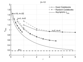
(a) $\beta=1/2$

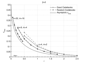
(b) $\beta=2$

Figure 1: $c_{\min,n}$

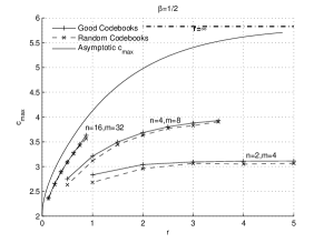
(a) $\beta=1/2$

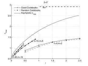
(b) $\beta=2$

Figure 2: $c_{\max,n}$

VI Conclusion

In this paper, we analyze the effect of finite rate feedback on CDMA signature optimization and MIMO beamforming vector selection. The main results are the exact asymptotic performance formulae. In addition, we prove that random codebooks are asymptotically optimal not only on average but also with probability one. The proofs rest on a large deviation principle derived over a random matrix ensemble.

-A Properties of Rate Functions

Let $Y$ be a non-negative random variable with probability measure $d\mu_{y}=e^{-y}dy$ for $y\in\left[0,+\infty\right)$. Let $Y_{M}$ be a non-negative random variable with probability measure

$$d\mu_{y,M}=\begin{cases}e^{-y}\frac{dy}{\mu_{Y}\left[0,M\right]}&\mathrm{if}\;y\in\left[0,M\right]\\ 0&\mathrm{otherwise}\end{cases}.$$ (15)

Let $d\mu_{\lambda}$ be (3). Define the moment generating functions

$$\psi_{x,M}\left(\alpha\right)\triangleq\int\log\mathrm{E}_{Y}\left[e^{\alpha\left(\lambda-x\right)Y},\left|Y\right|\leq M\right]d\mu_{\lambda},$$ (16)

$$\psi_{x}\left(\alpha\right)\triangleq\underset{M\rightarrow\infty}{\lim}\psi_{x,M}\left(\alpha\right),$$ (17)

and

$$\psi_{x,Y_{M}}\left(\alpha\right)\triangleq\int\log\mathrm{E}_{Y_{M}}\left[e^{\alpha\left(\lambda-x\right)Y_{M}}\right]d\mu_{\lambda}.$$ (18)

Clearly, $\psi_{x,Y_{M}}\left(\alpha\right)=\psi_{x,M}\left(\alpha\right)-\log\mu_{Y}\left[0,M\right].$ Proposition 2(3) shows that $\psi_{x}\left(\alpha\right)$ has the form (4). Furthermore, for $\forall t\in\mathbb{R}$, define the rate functions

$$\psi_{x}^{*}\left(t\right)\triangleq\underset{\alpha\in\mathbb{R}}{\sup}\left[\alpha t-\psi_{x}\left(\alpha\right)\right],$$ (19)

and

$$\psi_{x,Y_{M}}^{*}\left(t\right)\triangleq\underset{\alpha\in\mathbb{R}}{\sup}\left[\alpha t-\psi_{x,Y_{M}}\left(\alpha\right)\right].$$ (20)

In the following, we shall discuss the properties of these moment generating functions and rate functions.

Proposition 2

(Properties of $\psi\left(\cdot\right)$’s)

1. For $\forall\alpha\in\mathbb{R}$, $\log\mathrm{E}_{Y}\left[e^{\alpha\left(\lambda-x\right)Y},\left|Y\right|\leq M\right]$ is a Lipschitz function on any compact set of $\lambda\in\mathbb{R}$.

2. $\psi_{x,M}\left(\alpha\right)$ is monotonically increasing with $M$, and

   $$\psi_{x}\left(\alpha\right) \triangleq\underset{M\rightarrow\infty}{\lim}\psi_{x,M}\left(\alpha\right)$$

   $$=\begin{cases}-\int\log\left(1+\alpha\left(x-\lambda\right)\right)d\mu_{\lambda}&\mathrm{if}\;\alpha\in\left[-\frac{1}{x-\lambda_{t}^{-}},\frac{1}{\lambda^{+}-x}\right]\\ +\infty&\mathrm{otherwise}\end{cases}.$$

3. $\psi_{x,M}\left(\alpha\right)$ and $\psi_{x,Y_{M}}\left(\alpha\right)$ are strictly convex functions of $\alpha\in\mathbb{R}$, and $\psi_{x}\left(\alpha\right)$ is strictly convex on $\alpha\in\left(-\frac{1}{x-\lambda_{t}^{-}},\frac{1}{\lambda^{+}-x}\right)$.

4. Let $x\in\left(\lambda_{t}^{-},\lambda^{+}\right)$. For $\forall t<\bar{\lambda}-x$, if $M$ is large enough, there exists an $\alpha\in\left(-\infty,0\right)$ such that $\psi_{x,M}^{\prime}\left(\alpha\right)=\psi_{x,Y_{M}}^{\prime}\left(\alpha\right)=t$. Similarly, for $\forall t>\bar{\lambda}-x$, if $M$ is large enough, there exists an $\alpha\in\left(0,+\infty\right)$ such that $\psi_{x,M}^{\prime}\left(\alpha\right)=\psi_{x,Y_{M}}^{\prime}\left(\alpha\right)=t$.

Proof:

1. First note with the restriction $\{|Y|\leq M\}$, both $\log\mathrm{E}_{Y}\left[e^{\alpha\left(\lambda-x\right)Y},\left|Y\right|\leq M\right]$ and $\psi_{x,M}\left(\alpha\right)$ are well defined. Let $f_{M}\left(\lambda\right)=\log\int_{0}^{M}e^{\alpha\left(\lambda-x\right)y}e^{-y}dy$. Then

   $$f_{M}^{\prime}\left(\lambda\right)=\frac{\int_{0}^{M}\alpha ye^{\alpha\left(\lambda-x\right)y}e^{-y}dy}{\int_{0}^{M}e^{\alpha\left(\lambda-x\right)y}e^{-y}dy}.$$

   Since both $e^{\alpha\left(\lambda-x\right)y-y}$ and $\alpha ye^{\alpha\left(\lambda-x\right)y-y}$ are continuous functions of $\lambda$ and $y$ on the compact set $A_{\lambda}\times\left[0,M\right]$, and there exist positive constants $a>0$ and $b>0$ such that

   $$e^{\alpha\left(\lambda-x\right)y}e^{-y}\geq a,\ \ \mbox{ and }\ \ \left|\alpha ye^{\alpha\left(\lambda-x\right)y-y}\right|\leq b$$

   on that set. Thus, $\left|f_{M}^{\prime}\left(\lambda\right)\right|\leq\frac{b}{a}<\infty$ and so $f_{M}\left(\lambda\right)$ is Lipschitz on $A_{\lambda}$.

2. The monotonicity of $\psi_{x,M}\left(\alpha\right)$ is obvious, as is the identification of the limit $\psi_{x,M}\left(\alpha\right)$ presented in Part (3).

3. The convexity of logarithmic moment generating functions is a standard fact, see for example Chapter 2 of [11].

4. It is clear that $\psi_{x,M}^{\prime}\left(\alpha\right)=\psi_{x,Y_{M}}^{\prime}\left(\alpha\right)$, and we need only calculate the former.

   To simplify the notation, denote $z=1-\alpha\left(\lambda-x\right)$. Then

   $$\psi_{x,M}\left(\alpha\right)=\int\log\left(\frac{1-e^{-Mz}}{z}\right)d\mu_{\lambda}$$

   and

   $$\psi_{x,M}^{\prime}\left(\alpha\right) =\int\frac{1-\left(1+Mz\right)e^{-Mz}}{z\left(1-e^{-Mz}\right)}\left(\lambda-x\right)\cdot d\mu_{\lambda}.$$ (21)

   If $\alpha=0$, then $z\equiv 1$ and

   $$\psi_{x,M}^{\prime}\left(0\right)=\frac{1-\left(1+M\right)e^{-M}}{1-e^{-M}}\left(\bar{\lambda}-x\right).$$

   It is clear that

   $$\psi_{x,M}^{\prime}\left(0\right)\overset{M\rightarrow+\infty}{\longrightarrow}\bar{\lambda}-x.$$

   Now we evaluate $\psi_{x,M}^{\prime}\left(\pm\infty\right)$. Note that

   $$z=1-\alpha\left(\lambda-x\right)\overset{\alpha\rightarrow-\infty}{\longrightarrow}\begin{cases}-\infty&\mathrm{on}\;\lambda\in\left[\lambda_{t}^{-},x\right)\\ +\infty&\mathrm{on}\;\lambda\in\left(x,\lambda^{+}\right]\end{cases}.$$

   We evaluate the integrand in (21) and obtain that

   $$\frac{1-\left(1+Mz\right)e^{-Mz}}{z\left(1-e^{-Mz}\right)}\left(\lambda-x\right)\overset{\alpha\rightarrow-\infty}{\longrightarrow}\begin{cases}M\left(\lambda-x\right)&\mathrm{on}\;\lambda\in\left[\lambda_{t}^{-},x\right)\\ 0&\mathrm{on}\;\lambda\in\left(x,\lambda^{+}\right]\end{cases},$$

   and

   $$\frac{1-\left(1+Mz\right)e^{-Mz}}{z\left(1-e^{-Mz}\right)}\left(\lambda-x\right)\overset{\alpha\rightarrow+\infty}{\longrightarrow}\begin{cases}0&\mathrm{on}\;\lambda\in\left[\lambda_{t}^{-},x\right)\\ M\left(\lambda-x\right)&\mathrm{on}\;\lambda\in\left(x,\lambda^{+}\right]\end{cases}.$$

   Therefore,

   $$\psi_{x,M}^{\prime}\left(-\infty\right)\overset{M\rightarrow+\infty}{\longrightarrow}-\infty,$$

   and

   $$\psi_{x,M}^{\prime}\left(+\infty\right)\overset{M\rightarrow+\infty}{\longrightarrow}+\infty,$$

   which prove Part (5).

∎

Proposition 3

(Properties of $\psi_{x,Y_{M}}^{*}\left(\cdot\right)$)

1. $\psi_{x,Y_{M}}^{*}\left(t\right)\geq 0$.

2. For $\forall x\in\left(\lambda_{t}^{-},\lambda^{+}\right)$ and $\forall t\in\mathbb{R}$, if $M$ is large enough, there exists a $\gamma\in\mathbb{R}$ such that $\psi_{x,Y_{M}}^{\prime}\left(\gamma\right)=t$ and $\psi_{x,Y_{M}}^{*}\left(t\right)=\gamma t-\psi_{x,Y_{M}}\left(\gamma\right)$. More specifically, $\gamma<0$ when $t<\bar{\lambda}-x$, and $\gamma>0$ when $t>\bar{\lambda}-x$ .

3. Consider an $x\in\left(\lambda_{t}^{-},\lambda^{+}\right)$ and $\forall t_{1},t_{2}\in\mathbb{R}$. For a sufficiently large $M$, let $\psi_{x,Y_{M}}^{*}\left(t_{1}\right)$ and $\psi_{x,Y_{M}}^{*}\left(t_{2}\right)$ be achieved at $\alpha\in\mathbb{R}$ and $\beta\in\mathbb{R}$ respectively. Then

   $$\psi_{x,Y_{M}}^{*}\left(t_{2}\right)-\psi_{x,Y_{M}}^{*}\left(t_{1}\right)\leq\beta\left(t_{2}-t_{1}\right),$$

   where the equality holds if and only if $t_{1}=t_{2}$.

Proof:

1. It is from the fact that $\left.\alpha t-\psi_{x,Y_{M}}\left(\alpha\right)\right|_{\alpha=0}=0$.

2. This part follows directly from Proposition 2(5) and the strict convexity of $\psi_{x,Y_{M}}^{*}\left(t\right)$ (Proposition 2(4)).

3. Let $\alpha\in\mathbb{R}$ and $\gamma\in\mathbb{R}$ be such that $\psi_{x,Y_{M}}^{\prime}\left(\alpha\right)=t_{1}$ and $\psi_{x,Y_{M}}^{\prime}\left(\gamma\right)=t_{2}$. Clearly, $\psi_{x,Y_{M}}^{*}\left(t_{1}\right)=\alpha t_{1}-\psi_{x,Y_{M}}\left(\alpha\right)$ and $\psi_{x,Y_{M}}^{*}\left(t_{2}\right)=\gamma t_{2}-\psi_{x,Y_{M}}\left(\gamma\right)$. If $t_{1}\neq t_{2}$, then $\alpha\neq\gamma$ and

   $$\psi_{x,Y_{M}}^{*}\left(t_{2}\right)-\psi_{x,Y_{M}}^{*}\left(t_{1}\right) =\gamma t_{2}-\psi_{x,Y_{M}}\left(\gamma\right)-\left(\alpha t_{1}-\psi_{x,Y_{M}}\left(\alpha\right)\right)$$

   $$=\gamma\left(t_{2}-t_{1}\right)+t_{1}\left(\gamma-\alpha\right)-\left[\psi_{x,Y_{M}}\left(\gamma\right)-\psi_{x,Y_{M}}\left(\alpha\right)\right]$$

   $$\overset{\left(a\right)}{=}\gamma\left(t_{2}-t_{1}\right)+t_{1}\left(\gamma-\alpha\right)-\psi_{x,Y_{M}}^{\prime}\left(\xi\right)\left(\gamma-\alpha\right)$$

   $$=\gamma\left(t_{2}-t_{1}\right)+\left(t_{1}-\psi_{x,Y_{M}}^{\prime}\left(\xi\right)\right)\left(\gamma-\alpha\right)$$

   $$\overset{\left(b\right)}{<}\gamma\left(t_{2}-t_{1}\right),$$

   where $\left(a\right)$ is from the mean value theorem for some $\xi\in\left(\min\left(\alpha,\gamma\right),\max\left(\alpha,\gamma\right)\right)$, and $\left(b\right)$ follows from the strict convexity of $\psi_{x,Y_{M}}\left(\alpha\right)$.

∎

Proposition 4

(Properties of $\psi_{x}^{*}\left(0\right)$)

1. $\psi_{x}^{*}\left(t\right)\geq 0$.

2. Let $x\in\left(\lambda_{t}^{-},\lambda^{+}\right)$. For $\forall t<\bar{\lambda}-x$,

   $$\psi_{x}^{*}\left(t\right)=\underset{\alpha\in\left(-\frac{1}{x-\lambda_{t}^{-}},0\right)}{\sup}\;\alpha t-\psi_{x}\left(\alpha\right).$$

   For $\forall t>\bar{\lambda}-x$,

   $$\psi_{x}^{*}\left(t\right)=\underset{\alpha\in\left(0,\frac{1}{\lambda^{+}-x}\right)}{\sup}\;\alpha t-\psi_{x}\left(\alpha\right).$$

3. $\psi_{\bar{\lambda}}^{*}\left(0\right)=0$.

4. $\psi_{x}^{*}\left(0\right)$ monotonically decreases on $x\in\left(\lambda_{t}^{-},\bar{\lambda}\right)$ and monotonically increases on $x\in\left(\bar{\lambda},\lambda^{+}\right)$.

5. As $x\downarrow\lambda_{t}^{-}$ or $x\uparrow\lambda^{+}$, $\psi_{x}^{*}\left(0\right)\rightarrow+\infty$.

6. For $\forall r\in\mathbb{R}^{+}$, there are unique $x_{r}^{-}\in\left(\lambda_{t}^{-},\bar{\lambda}\right)$ and $x_{r}^{+}\in\left(\bar{\lambda},\lambda^{+}\right)$ such that $r\log 2=\psi_{x_{r}^{-}}^{*}\left(0\right)=\psi_{x_{r}^{+}}^{*}\left(0\right)$.

Proof:

1. It is from the fact that $\left.\alpha t-\psi_{x}\left(\alpha\right)\right|_{\alpha=0}=0$.

2. We only prove it for the case that $t<\bar{\lambda}-x$, as $t>\bar{\lambda}-x$ is the dual case.

   It is clear that

   $$\psi_{x}^{*}\left(t\right)=\underset{\alpha\in\left[-\frac{1}{x-\lambda_{t}^{-}},\frac{1}{\lambda^{+}-x}\right]}{\sup}\;\alpha t-\psi_{x}\left(\alpha\right)$$

   for $\psi_{x}\left(\alpha\right)=+\infty$ if $\alpha\notin\left[-\frac{1}{x-\lambda_{t}^{-}},\frac{1}{\lambda^{+}-x}\right]$. Now for any $\alpha>0$,

   $$\alpha t-\int\log\mathrm{E}_{Y}\left[e^{\alpha\left(\lambda-x\right)Y}\right]d\mu_{\lambda}$$

   $$\leq\alpha t-\int\mathrm{E}_{Y}\left[\log e^{\alpha\left(\lambda-x\right)Y}\right]d\mu_{\lambda}$$

   $$=\alpha\left(t-\left(\bar{\lambda}-x\right)\right)$$

   $$<0.$$

   Note that $\psi_{x}^{*}\left(t\right)\geq 0$, the $\sup$ is on $\alpha\in\left[-\frac{1}{x-\lambda_{t}^{-}},0\right]$. Since $\log\left(1+\alpha\left(x-\lambda\right)\right)$ is continuous on $\alpha\in\left(-\frac{1}{x-\lambda_{t}^{-}},0\right)$, it is sufficient to have the sup on $\alpha\in\left(-\frac{1}{x-\lambda_{t}^{-}},0\right)$.

3. $\psi_{\bar{\lambda}}^{*}\left(0\right)\geq 0$ by Part (1). However, $\psi_{\bar{\lambda}}\left(\alpha\right)\geq-\log\left(1+\alpha\left(\bar{\lambda}-\bar{\lambda}\right)\right)=0$ and $\psi_{x}^{*}\left(t\right)=-\underset{\alpha\in\mathbb{R}}{\inf}\;\psi_{x}\left(\alpha\right)\leq 0$. We have that $\psi_{\bar{\lambda}}^{*}\left(0\right)=0$.

4. If $\lambda_{t}^{-}<y<x<\bar{\lambda}$,

   $$\psi_{y}^{*}\left(0\right) =\underset{\alpha\in\left(-\frac{1}{y-\lambda_{t}^{-}},0\right)}{\sup}\;\int_{\lambda_{t}^{-}}^{\lambda^{+}}\log\left(1+\alpha\left(y-\lambda\right)\right)d\mu_{\lambda}$$

   $$\overset{\left(a\right)}{\geq}\underset{\alpha\in\left(-\frac{1}{x-\lambda_{t}^{-}},0\right)}{\sup}\;\int_{\lambda_{t}^{-}}^{\lambda^{+}}\log\left(1+\alpha\left(y-\lambda\right)\right)d\mu_{\lambda}$$

   $$\overset{\left(b\right)}{>}\underset{\alpha\in\left(-\frac{1}{x-\lambda_{t}^{-}},0\right)}{\sup}\;\int_{\lambda_{t}^{-}}^{\lambda^{+}}\log\left(1+\alpha\left(x-\lambda\right)\right)d\mu_{\lambda}$$

   $$=\psi_{x}^{*}\left(0\right),$$

   where $\left(a\right)$ follows from shrinking the range of $\alpha$, and $\left(b\right)$ is from the facts that $y-\lambda<x-\lambda$ and $\alpha<0$.

   Similarly, if $\bar{\lambda}<x<y<\lambda^{+}$, $\psi_{y}^{*}\left(0\right)>\psi_{x}^{*}\left(0\right)$.

5. In order to prove that $x\downarrow\lambda_{t}^{-}$ implies $\psi_{x}^{*}\left(0\right)\uparrow\infty$, let $x_{n}\downarrow\lambda_{t}^{-}$ and $\alpha_{n}=-\frac{1}{2\left(x_{n}-\lambda_{t}^{-}\right)}\in\left(-\frac{1}{x_{n}-\lambda_{t}^{-}},0\right)$. Then $\psi_{x_{n}}\left(\alpha_{n}\right)$ is well defined for all $n$.

   $$\psi_{x_{n}}^{*}\left(0\right)\geq\psi_{x_{n}}\left(\alpha_{n}\right)=\int\log\left(\frac{x_{n}-\lambda_{t}^{-}+\lambda-\lambda_{t}^{-}}{2\left(x_{n}-\lambda_{t}^{-}\right)}\right)d\mu_{\lambda}.$$

   We shall show that $\psi_{x_{n}}^{*}\left(\alpha_{n}\right)\uparrow\infty$.

   When $\beta\leq 1$ $\left(\lambda_{t}^{-}=\lambda^{-}\geq 0\right)$,

   $$\psi_{x_{n}}\left(\alpha_{n}\right) =\int\log\left(x_{n}-\lambda_{t}^{-}+\lambda-\lambda_{t}^{-}\right)d\mu_{\lambda}-\log 2-\log\left(x_{n}-\lambda_{t}^{-}\right).$$

   Since for $\epsilon>0$, $\left|\int_{0}^{\epsilon}x^{a+1}\log\left(x\right)dx\right|<\infty$ for $\forall a>-1$, and we have $\left|\int\log\left(\lambda-\lambda^{-}\right)d\mu_{\lambda}\right|<\infty$, it holds

   $$\psi_{x_{n}}\left(\alpha_{n}\right)\geq\int\log\left(\lambda-\lambda_{t}^{-}\right)d\mu_{\lambda}-\log\left(x_{n}-\lambda_{t}^{-}\right)-const.\overset{n\rightarrow\infty}{\rightarrow}+\infty.$$

   When $\beta>1$ $\left(\lambda_{t}^{-}=0,\;\lambda^{-}>0\right)$,

   $$\psi_{x_{n}}\left(\alpha_{n}\right) =\frac{\tau-1}{\tau}\log\frac{1}{2}+\frac{1}{\tau}\int_{\lambda^{-}}^{\lambda^{+}}\log\left(\frac{x_{n}+\lambda}{2x_{n}}\right)\frac{\left(\lambda-\lambda^{-}\right)^{1/2}\left(\lambda^{+}-\lambda\right)^{\frac{1}{2}}}{2\pi\lambda}d\lambda$$

   $$=\frac{\tau-1}{\tau}\log\frac{1}{2}-\frac{1}{\tau}\log\left(2x_{n}\right)+\frac{1}{\tau}\int_{\lambda^{-}}^{\lambda^{+}}\log\left(x_{n}+\lambda\right)\frac{\left(\lambda-\lambda^{-}\right)^{1/2}\left(\lambda^{+}-\lambda\right)^{\frac{1}{2}}}{2\pi\lambda}d\lambda$$

   $$\overset{n\rightarrow\infty}{\longrightarrow}\infty.$$

   Similarly, let $x_{n}\uparrow\lambda^{+}$ and $\alpha_{n}=\frac{1}{2\left(\lambda^{+}-x\right)}\in\left(0,\frac{1}{\lambda^{+}-x}\right)$. It can be proved that as $n\rightarrow\infty$ , $\psi_{x_{n}}\left(\alpha_{n}\right)\rightarrow\infty$ and therefore $\psi_{x_{n}}^{*}\left(0\right)\rightarrow\infty$.

6. This follows from Prop. 3 (5) and (6).

∎

-B Large Deviation Principles

This section is devoted to prove the following large deviation principle for $\mu_{n,\mathbf{Y}}$.

Theorem 5

Let $n,m\rightarrow\infty$ with $\frac{m}{n}\rightarrow\frac{1}{\beta}\in\mathbb{R}^{+}$. For any $t<\bar{\lambda}-x$,

$$\underset{\left(n,m\right)\rightarrow\infty}{\lim}\frac{1}{n}\log\mu_{n,\mathbf{Y}}\left(\left.\frac{1}{n}\sum_{i=1}^{n}\left(\lambda_{i}-x\right)Y_{i}\leq t\right|\bm{\lambda}\right)=-\psi_{x}^{*}\left(t\right)=-\underset{\alpha<0}{\sup}\left[\alpha t-\psi_{x}\left(\alpha\right)\right]$$

almost surely (in $\bm{\lambda}$). Similarly, for any $t>\bar{\lambda}-x$,

$$\underset{\left(n,m\right)\rightarrow\infty}{\lim}\frac{1}{n}\log\mu_{n,\mathbf{Y}}\left(\left.\frac{1}{n}\sum_{i=1}^{n}\left(\lambda_{i}-x\right)Y_{i}\geq t\right|\bm{\lambda}\right)=-\psi_{x}^{*}\left(t\right)=-\underset{\alpha>0}{\sup}\left[\alpha t-\psi_{x}\left(\alpha\right)\right]$$

almost surely (in $\bm{\lambda}$).

The proof of Theorem 5 rests on another large deviation principle presented in below. Recall the truncated variable $Y_{M}$ defined in (15), its moment generating function $\psi_{x,Y_{M}}\left(\alpha\right)$ in (18) and its rate function $\psi_{x,Y_{M}}^{*}\left(t\right)$ in (20).

Theorem 6

Let $n,m\rightarrow\infty$ with $\frac{m}{n}\rightarrow\frac{1}{\beta}\in\mathbb{R}^{+}$. For any $t<\bar{\lambda}-x$ and large enough $M$,

$$\underset{\left(n,m\right)\rightarrow\infty}{\lim}\frac{1}{n}\log\mu_{n,\mathbf{Y}_{M}}\left(\left.\frac{1}{n}\sum_{i=1}^{n}\left(\lambda_{i}-x\right)Y_{M,i}\leq t\right|\bm{\lambda}\right)=-\psi_{x,Y_{M}}^{*}\left(t\right)=-\underset{\alpha<0}{\sup}\left[\alpha t-\psi_{x,Y_{M}}\left(\alpha\right)\right]$$

almost surely (in $\bm{\lambda}$). Similarly, for any $t>\bar{\lambda}-x$ and sufficiently large $M$,

$$\underset{\left(n,m\right)\rightarrow\infty}{\lim}\frac{1}{n}\log\mu_{n,\mathbf{Y}_{M}}\left(\left.\frac{1}{n}\sum_{i=1}^{n}\left(\lambda_{i}-x\right)Y_{M,i}\geq t\right|\bm{\lambda}\right)=-\psi_{x,Y_{M}}^{*}\left(t\right)=-\underset{\alpha>0}{\sup}\left[\alpha t-\psi_{x,Y_{M}}\left(\alpha\right)\right]$$

almost surely (in $\bm{\lambda}$).

The proof of Theorem 6 is given in Appendix -B2. Based on Theorem 6, Theorem 5 is proved in Appendix -B1.

-B1 Proof of Theorem 5

In the following, we only prove Theorem 6 for $t<\bar{\lambda}-x$. The $t>\bar{\lambda}-x$ case is just the dual case.

An upper bound is constructed by Chebyshev inequality. Take any $\alpha\in\left(-\frac{1}{x-\lambda_{t}^{-}},0\right)$,

$$\underset{\left(n,m\right)\rightarrow\infty}{\lim}\frac{1}{n}\log\mu_{n,\mathbf{Y}}\left(\left.\frac{1}{n}\sum_{i=1}^{n}\left(\lambda_{i}-x\right)Y_{i}\leq t\right|\bm{\lambda}\right)$$

$$\leq\underset{\left(n,m\right)\rightarrow\infty}{\lim}\frac{1}{n}\log\left\{e^{-n\alpha t}\mathrm{E}_{\mathbf{Y}}\left[\left.e^{\alpha\sum_{i=1}^{n}\left(\lambda_{i}-x\right)Y_{i}}\right|\bm{\lambda}\right]\right\}$$

$$=-\left\{\alpha t-\int\log\mathrm{E}_{Y}\left[e^{\alpha\left(\lambda-x\right)Y}\right]d\mu_{\lambda}\right\}$$

almost surely (in $\bm{\lambda}$), where the last equality follows from the fact that $\mathrm{E}_{Y}\left[e^{\alpha\left(\lambda-x\right)Y}\right]$ is Lipschitz on $\left[\lambda_{t}^{-},\lambda^{+}\right]$ for $\forall\alpha\in\left(-\frac{1}{x-\lambda_{t}^{-}},0\right)$. Therefore,

$$\underset{\left(n,m\right)\rightarrow\infty}{\lim}\frac{1}{n}\log\mu_{n,\mathbf{Y}}\left(\left.\frac{1}{n}\sum_{i=1}^{n}\left(\lambda_{i}-x\right)Y_{i}\leq t\right|\bm{\lambda}\right)$$

$$\leq-\underset{\alpha\in\left(-\frac{1}{x-\lambda_{t}^{-}},0\right)}{\sup}\left\{\alpha t-\psi_{x}\left(\alpha\right)\right\}=-\psi_{x}^{*}\left(t\right)$$ (22)

almost surely (in $\bm{\lambda}$), where the last equality follows from Proposition 4(2).

A lower bound is obtained from Theorem 6.

$$\underset{\left(n,m\right)\rightarrow\infty}{\lim}\frac{1}{n}\log\mu_{n,\mathbf{Y}}\left(\left.\frac{1}{n}\sum_{i=1}^{n}\left(\lambda_{i}-x\right)Y_{i}\leq t\right|\bm{\lambda}\right)$$

$$\geq\underset{\left(n,m\right)\rightarrow\infty}{\lim}\frac{1}{n}\log\mu_{n,\mathbf{Y}}\left(\left.\frac{1}{n}\sum_{i=1}^{n}\left(\lambda_{i}-x\right)Y_{i}\leq t,\;\cap_{i=1}^{n}\left\{\left|Y_{i}\right|\leq M\right\}\right|\bm{\lambda}\right)$$

$$=\underset{\left(n,m\right)\rightarrow\infty}{\lim}\frac{1}{n}\log\mu_{n,\mathbf{Y}_{M}}\left(\left.\frac{1}{n}\sum_{i=1}^{n}\left(\lambda_{i}-x\right)Y_{i}\leq t\right|\bm{\lambda}\right)-\log\mu_{Y}\left[0,M\right]$$

$$=-\psi_{x,Y_{M}}^{*}\left(t\right)-\log\mu_{Y}\left[0,M\right],$$

almost surely in $\bm{\lambda}$. where the last equality follows from Theorem 6. Note that $\psi_{x}\left(\alpha\right)=\underset{M\rightarrow\infty}{\lim}\psi_{x,Y_{M}}\left(\alpha\right)$, $\psi_{x}^{*}\left(t\right)=\underset{M\rightarrow\infty}{\lim}\psi_{x,Y_{M}}^{*}\left(t\right)$ and $\underset{M\rightarrow\infty}{\lim}\log\mu_{Y}\left[0,M\right]=0$.

$$\underset{\left(n,m\right)\rightarrow\infty}{\lim}\frac{1}{n}\log\mu_{n,\mathbf{Y}}\left(\left.\frac{1}{n}\sum_{i=1}^{n}\left(\lambda_{i}-x\right)Y_{i}\leq t\right|\bm{\lambda}\right)\geq-\psi_{x}^{*}\left(t\right)$$

almost surely in $\bm{\lambda}$, which proves Theorem 5.

-B2 Proof of Theorem 6

The proof of this theorem follows the same line in that of Gartner-Ellis Theorem [11]. In the following, we only gives the details for $t<\bar{\lambda}-x$, as the $t>\bar{\lambda}-x$ case is just the dual case.

Similar to the upper bound in (22), by Chebyshev’s inequality and maximization over $\alpha\in\mathbb{R}^{-}$, we have the upper bound

$$\underset{\left(n,m\right)\rightarrow\infty}{\lim}\frac{1}{n}\log\mu_{n,\mathbf{Y}_{M}}\left(\left.\frac{1}{n}\sum_{i=1}^{n}\left(\lambda_{i}-x\right)Y_{M,i}\leq t\right|\bm{\lambda}\right)$$

$$\leq-\underset{\alpha<0}{\sup}\left[\alpha t-\psi_{x,Y_{M}}\left(\alpha\right)\right]$$

$$=\psi_{x,Y_{M}}^{*}\left(t\right)$$

almost surely in $\bm{\lambda}$, where the last equality follows from Proposition 3(2).

Now we prove the lower bound

$$\underset{\left(n,m\right)\rightarrow\infty}{\lim}\frac{1}{n}\log\mu_{n,\mathbf{Y}_{M}}\left(\left.\frac{1}{n}\sum_{i=1}^{n}\left(\lambda_{i}-x\right)Y_{M,i}\leq t\right|\bm{\lambda}\right)\geq-\psi_{x,Y_{M}}^{*}\left(t\right)$$ (23)

almost surely in $\bm{\lambda}$. This lower bound rests on the fact (will be proved later) that for any $s\in\mathbb{R}$ and $\epsilon>0$,

$$\underset{\left(n,m\right)\rightarrow\infty}{\lim}\frac{1}{n}\log\mu_{n,\mathbf{Y}_{M}}\left(\left.\frac{1}{n}\sum_{i=1}^{n}\left(\lambda_{i}-x\right)Y_{M,i}\in\left(s-\epsilon,s+\epsilon\right)\right|\bm{\lambda}\right)\geq-\psi_{x,Y_{M}}^{*}\left(s\right)$$ (24)

almost surely in $\bm{\lambda}$. Note that for $\forall s<t$, there exists an $\epsilon>0$ such that $\left(s-\epsilon,s+\epsilon\right)\subset\left(-\infty,t\right)$ and

$$\underset{\left(n,m\right)\rightarrow\infty}{\lim}\frac{1}{n}\log\mu_{n,\mathbf{Y}_{M}}\left(\left.\frac{1}{n}\sum_{i=1}^{n}\left(\lambda_{i}-x\right)Y_{M,i}\leq t\right|\bm{\lambda}\right)$$

$$\geq\underset{\left(n,m\right)\rightarrow\infty}{\lim}\frac{1}{n}\log\mu_{n,\mathbf{Y}_{M}}\left(\left.\frac{1}{n}\sum_{i=1}^{n}\left(\lambda_{i}-x\right)Y_{M,i}\in\left(s-\epsilon,s+\epsilon\right)\right|\bm{\lambda}\right)$$

$$\geq-\psi_{x,Y_{M}}^{*}\left(s\right)$$

almost surely in $\bm{\lambda}$. Take $s\uparrow t$. $\psi_{x,Y_{M}}^{*}\left(s\right)\rightarrow\psi_{x,Y_{M}}^{*}\left(t\right)$. The lower bound (23) is then proved.

The inequality (24) is proved by exponential change of measure. Let $\gamma\in\mathbb{R}$ such that $\psi_{x,Y_{M}}^{*}\left(s\right)=\gamma s-\psi_{x,Y_{M}}\left(\gamma\right)$, or equivalently, $\psi_{x,Y_{M}}^{\prime}\left(\gamma\right)=s$. Such $\gamma$ exists according to Proposition 3(2). Note that $d\mu_{n,\mathbf{y}_{M}}=\prod_{i=1}^{n}d\mu_{y_{M,i}}.$ Define a new probability measure (exponential change of $d\mu_{n,\mathbf{y}_{m}}$)

$$d\tilde{\mu}_{n,\mathbf{y}_{M}} \triangleq\frac{e^{\sum_{i=1}^{n}\gamma\left(\lambda_{i}-x\right)y_{i}}}{\mathrm{E}_{\mathbf{Y}_{M}}\left[e^{\sum_{i=1}^{n}\gamma\left(\lambda_{i}-x\right)Y_{M,i}}\right]}d\mu_{n,\mathbf{y}_{M}}$$

$$=\frac{e^{\sum_{i=1}^{n}\gamma\left(\lambda_{i}-x\right)y_{i}}}{e^{\sum_{i=1}^{n}\log\mathrm{E}_{Y_{M}}\left[e^{\gamma\left(\lambda_{i}-x\right)Y_{M}}\right]}}d\mu_{n,\mathbf{y}_{M}}.$$

Since $\int d\tilde{\mu}_{n,\mathbf{y}_{M}}=1$, $\tilde{\mu}_{n,\mathbf{y}_{M}}$ is a well defined probability measure. Let

$$A_{n,\mathbf{y}}\triangleq\left\{\left(y_{1},\cdots,y_{n}\right):\;\mathbf{y}\in\prod_{i=1}^{n}\left[0,M\right],\;\frac{1}{n}\sum_{i=1}^{n}\left(\lambda_{i}-x\right)y_{i}\in\left(s-\epsilon,s+\epsilon\right)\right\}.$$

Then

$$\frac{1}{n}\log\mu_{n,\mathbf{Y}_{M}}\left(\left.\sum_{i=1}^{n}\left(\lambda_{i}-x\right)Y_{M,i}\in\left(s-\epsilon,s+\epsilon\right)\right|\bm{\lambda}\right)$$

$$=\frac{1}{n}\log\int_{A_{n,\mathbf{y}}}d\mu_{n,\mathbf{y}_{M}}$$

$$=\frac{1}{n}\log\int_{A_{n,\mathbf{y}}}\left(e^{\sum_{i=1}^{n}\log\mathrm{E}_{Y_{M}}\left[\left.e^{\gamma\left(\lambda_{i}-x\right)Y_{M}}\right|\bm{\lambda}\right]}\cdot e^{-\sum_{i=1}^{n}\gamma\left(\lambda_{i}-x\right)y_{i}}\right)d\tilde{\mu}_{n,\mathbf{y}_{M}}$$

$$=\frac{1}{n}\log e^{-n\left\{\gamma s-\frac{1}{n}\sum_{i=1}^{n}\log\mathrm{E}_{Y_{M}}\left[\left.e^{\gamma\left(\lambda_{i}-x\right)Y_{M}}\right|\bm{\lambda}\right]\right\}}$$

$$\quad\quad+\frac{1}{n}\log\int_{A_{n,\mathbf{y}}}e^{-n\gamma\left[\frac{1}{n}\sum_{i=1}^{n}\left(\lambda_{i}-x\right)y_{i}-s\right]}d\tilde{\mu}_{n,\mathbf{y}_{M}}$$

$$\geq-\left\{\gamma s-\frac{1}{n}\sum_{i=1}^{n}\log\mathrm{E}_{Y_{M}}\left[\left.e^{\gamma\left(\lambda_{i}-x\right)Y_{M}}\right|\bm{\lambda}\right]\right\}+\frac{1}{n}\log\left(e^{-n\left|\gamma\epsilon\right|}\int_{A_{n,\mathbf{y}}}d\tilde{\mu}_{n,\mathbf{y}_{M}}\right)$$

$$=-\left\{\gamma s-\frac{1}{n}\sum_{i=1}^{n}\log\mathrm{E}_{Y_{M}}\left[\left.e^{\gamma\left(\lambda_{i}-x\right)Y_{M}}\right|\bm{\lambda}\right]\right\}-\left|\gamma\epsilon\right|+\frac{1}{n}\log\tilde{\mu}_{n,\mathbf{Y}_{M}}\left(\left.A_{n,\mathbf{y}}\right|\bm{\lambda}\right).$$

Note that $\underset{\left(n,m\right)\rightarrow\infty}{\lim}\;\frac{1}{n}\sum_{i=1}^{n}\log\mathrm{E}_{Y_{M}}\left[\left.e^{\gamma\left(\lambda_{i}-x\right)Y_{M}}\right|\bm{\lambda}\right]=\psi_{x,Y_{M}}\left(\gamma\right)$ almost surely in $\bm{\lambda}$. (24) is true if

$$\underset{\left(n,m\right)\rightarrow\infty}{\lim}\frac{1}{n}\log\tilde{\mu}_{n,\mathbf{Y}_{M}}\left(\left.A_{n,\mathbf{y}}\right|\bm{\lambda}\right)=0$$ (25)

almost surely in $\bm{\lambda}$.

In order to prove (25), note that

$$\tilde{\mu}_{n,\mathbf{Y}_{M}}\left(\left.A_{n,\mathbf{y}}\right|\bm{\lambda}\right) =1-\tilde{\mu}_{n,\mathbf{Y}_{M}}\left(\left.\frac{1}{n}\sum_{i=1}^{n}\left(\lambda_{i}-x\right)y_{i}\leq s-\epsilon\right|\bm{\lambda}\right)$$

$$\quad\quad-\tilde{\mu}_{n,\mathbf{Y}_{M}}\left(\left.\frac{1}{n}\sum_{i=1}^{n}\left(\lambda_{i}-x\right)y_{i}\geq s+\epsilon\right|\bm{\lambda}\right).$$

We upper bound $\tilde{\mu}_{n,\mathbf{Y}_{M}}\left(\left.\frac{1}{n}\sum_{i=1}^{n}\left(\lambda_{i}-x\right)y_{i}\leq s-\epsilon\right|\bm{\lambda}\right)$ and $\tilde{\mu}_{n,\mathbf{Y}_{M}}\left(\left.\frac{1}{n}\sum_{i=1}^{n}\left(\lambda_{i}-x\right)y_{i}\geq s+\epsilon\right|\bm{\lambda}\right)$ respectively. Note that

$$\underset{\left(n,m\right)\rightarrow\infty}{\lim}\frac{1}{n}\log\int e^{\alpha\sum\left(\lambda_{i}-x\right)y_{i}}d\tilde{\mu}_{n,\mathbf{y}_{M}}$$

$$=\underset{\left(n,m\right)\rightarrow\infty}{\lim}\left[\frac{1}{n}\log\int e^{\left(\alpha+\gamma\right)\sum\left(\lambda_{i}-x\right)y_{i}}d\mu_{n,\mathbf{y}_{M}}-\frac{1}{n}\log\mathrm{E}_{\mathbf{Y}_{M}}\left[\left.e^{\gamma\sum\left(\lambda_{i}-x\right)Y_{M,i}}\right|\bm{\lambda}\right]\right]$$

$$=\psi_{x,Y_{M}}\left(\alpha+\gamma\right)-\psi_{x,Y_{M}}\left(\gamma\right)$$

almost surely in $\bm{\lambda}$. Define $\tilde{\psi}_{x,Y_{M}}\left(\alpha\right)=\psi_{x,Y_{M}}\left(\alpha+\gamma\right)-\psi_{x,Y_{M}}\left(\gamma\right)$ and $\tilde{\psi}_{x,Y_{M}}^{*}\left(s\right)=\underset{\alpha}{\sup}\left[\alpha s-\tilde{\psi}_{x,Y_{M}}\left(\alpha\right)\right]$. Since $\psi_{x,Y_{M}}\left(\alpha\right)$ is strictly convex (Proposition 2(4)), $\tilde{\psi}_{x,Y_{M}}\left(\alpha\right)$ is strictly convex. Note that $\psi_{x,Y_{M}}^{\prime}\left(\gamma\right)=s$ as $M$ is sufficiently large. For large enough $M$,

$$\tilde{\psi}_{x,Y_{M}}^{\prime}\left(\alpha\right)=\psi_{x,Y_{M}}^{\prime}\left(\alpha+\gamma\right)\begin{cases}>s&\mathrm{if}\;\alpha>0\\ =s&\mathrm{if}\;\alpha=0\\ <s&\mathrm{if}\;\alpha<0\end{cases}.$$

Therefore, $\tilde{\psi}_{x,Y_{M}}^{*}\left(s-\epsilon\right)$ is achieved at an $\alpha_{s-\epsilon}<0$ and

$$\tilde{\psi}_{x,Y_{M}}^{*}\left(s-\epsilon\right) =\alpha_{s-\epsilon}\left(s-\epsilon\right)-\tilde{\psi}_{x,Y_{M}}\left(\alpha_{s-\epsilon}\right)$$

$$=\left(\alpha_{s-\epsilon}+\gamma\right)\left(s-\epsilon\right)-\psi_{x,Y_{M}}\left(\alpha_{s-\epsilon}+\gamma\right)-\gamma s+\psi_{x,Y_{M}}\left(\gamma\right)+\gamma\epsilon$$

$$\overset{\left(a\right)}{=}\gamma\epsilon-\left[\psi_{x,Y_{M}}^{*}\left(s\right)-\psi_{x,Y_{M}}^{*}\left(s-\epsilon\right)\right]$$

$$\overset{\left(b\right)}{>}0,$$

where $\left(a\right)$ is from the fact that $\psi_{x,Y_{M}}^{\prime}\left(\alpha_{t-\epsilon}+\gamma\right)=t-\epsilon$, and $\left(b\right)$ follows from Proposition 3(3). Similarly, $\tilde{\psi}_{x,Y_{M}}^{*}\left(s+\epsilon\right)$ is achieved at an $\alpha_{s+\epsilon}>0$ and $\tilde{\psi}_{x}^{*}\left(ts+\epsilon\right)>0$. Now, by Chebyshev’s inequality,

$$\underset{\left(n,m\right)\rightarrow\infty}{\lim}\frac{1}{n}\log\tilde{\mu}_{n,\mathbf{Y}_{M}}\left(\left.\frac{1}{n}\sum\left(\lambda_{i}-x\right)\tilde{Y}_{M,i}\leq s-\epsilon\right|\bm{\lambda}\right)=-\tilde{\psi}_{x,Y_{M}}^{*}\left(s-\epsilon\right)<0,$$

and

$$\underset{\left(n,m\right)\rightarrow\infty}{\lim}\frac{1}{n}\log\tilde{\mu}_{n,\mathbf{Y}_{M}}\left(\left|\frac{1}{n}\sum\left(\lambda_{i}-x\right)\tilde{Y}_{M,i}\leq s-\epsilon\right|\bm{\lambda}\right)=-\tilde{\psi}_{x,Y_{M}}^{*}\left(s+\epsilon\right)<0.$$

almost surely in $\bm{\lambda}$. Take a $b>0$ such that $\tilde{\psi}_{x}^{*}\left(t-\epsilon\right)>b$ and $\tilde{\psi}_{x}^{*}\left(t+\epsilon\right)>b$. Then,

$$\underset{\left(n,m\right)\rightarrow\infty}{\lim}\frac{1}{n}\log\tilde{\mu}_{n,\mathbf{Y}_{M}}\left(\left.A_{n,\mathbf{y}}\right|\bm{\lambda}\right)$$

$$\geq\underset{\left(n,m\right)\rightarrow\infty}{\lim}\frac{1}{n}\log\left(1-2e^{-nb\left(1+o\left(1\right)\right)}\right)=0,$$

which is exactly (25).

-C Proof of Corollary 1

The following lemma, proved in [10], is essential to our derivation in Corollary 1.

Lemma 3

For $\forall z\in\mathbb{C}\backslash\left[\lambda^{-},\lambda^{+}\right]$,

$$\int_{0}^{\infty}\frac{z\lambda}{1+z\lambda}f_{\beta}\left(\lambda\right)d\lambda=\frac{\mathcal{F}\left(z,\beta\right)}{4z\beta},$$ (26)

and

$$\int_{0}^{\infty}\log\left(1+z\lambda\right)f_{\beta}\left(\lambda\right)d\lambda=\log\left(1+z-\frac{1}{4}\mathcal{F}\left(z,\beta\right)\right)+\frac{1}{\beta}\log\left(1+z\beta-\frac{1}{4}\mathcal{F}\left(z,\beta\right)\right)-\frac{\mathcal{F}\left(z,\beta\right)}{4z\beta},$$ (27)

where

$$\mathcal{F}\left(z,\beta\right)\triangleq\left(\left(1+\lambda^{-}z\right)^{1/2}-\left(1+\lambda^{+}z\right)^{1/2}\right)^{2}.$$

The basic step uses (26) to identify the $\alpha^{*}$ at which $\psi_{x}^{*}\left(0\right)$ is achieved.

Proposition 5

Let $x\in\left(\lambda_{t}^{-},\lambda^{+}\right)$. Let $\alpha^{*}$ be such that $\psi_{x}^{*}\left(0\right)=\int\log\left(1+\alpha^{*}\left(x-\lambda\right)\right)d\mu_{\lambda}$. Then

$$\alpha^{*}=\begin{cases}\frac{1}{\lambda^{+}-x}&\mathrm{if}\;x\geq 1+\sqrt{\beta},\\ -\frac{1}{x-\lambda^{-}}&\mathrm{if}\;x\leq 1-\sqrt{\beta}\;\mathrm{and}\;\beta<1,\\ \frac{1}{\beta}\frac{x-1}{x}&\mathrm{otherwise}.\end{cases}$$

Proof:

Since $-\psi_{x}\left(\alpha\right)=\int\log\left(1+\alpha\left(x-\lambda\right)\right)d\mu_{\lambda}$ is concave on $\alpha\in\left(-\frac{1}{x-\lambda_{t}^{-}},\frac{1}{\lambda^{+}-x}\right)$ (Proposition 2(4)), $\alpha^{*}$ can be found by evaluating $-\psi_{x}^{\prime}\left(\alpha\right)$.

We computes $-\psi_{x}^{\prime}\left(\alpha\right)$ for any $\alpha\neq-\frac{1}{x},$

$$\int\frac{x-\lambda}{1+\alpha\left(x-\lambda\right)}d\mu_{\lambda}$$

$$=\frac{1}{\alpha}\left[\frac{\alpha x}{1+\alpha x}+\frac{1}{1+\alpha x}\int\frac{-\frac{\alpha}{1+\alpha x}\lambda}{1-\frac{\alpha}{1+\alpha x}\lambda}d\mu_{\lambda}\right]$$

$$=\frac{1}{\alpha}\left[\frac{\alpha x}{1+\alpha x}-\frac{\mathcal{F}\left(-\frac{\alpha}{1+\alpha x},\beta\right)}{4\alpha\beta}\right],$$ (28)

where the last line follows from (26).

By evaluating $\psi_{x}^{\prime}\left(\alpha\right)$ at the boundary points $\alpha=\frac{1}{\lambda^{+}-x}$ and $\alpha=-\frac{1}{x-\lambda_{t}^{-}}$, it can be verified that $\alpha^{*}$ satisfies

$$\begin{cases}\alpha^{*}=-\frac{1}{x-\lambda^{-}}&\mathrm{if}\;x<1-\sqrt{\beta}\;\mathrm{and}\;\beta<1\\ \alpha^{*}=\frac{1}{\lambda^{+}-x}&\mathrm{if}\;x>1+\sqrt{\beta}\\ \psi_{x}^{\prime}\left(\alpha^{*}\right)=0&\mathrm{otherwise}\end{cases}.$$

We shall find $\alpha\in\left(-\frac{1}{x-\lambda_{t}^{-}},\frac{1}{\lambda^{+}-x}\right)$ such that $\psi_{x}^{\prime}\left(\alpha\right)=0$. Suppose that $\alpha\neq-\frac{1}{x}$ where $\psi_{x}^{\prime}\left(\alpha\right)$ can be computed from (28). $\psi_{x}^{\prime}\left(\alpha\right)=0$ implies $\mathcal{F}\left(-\frac{\alpha}{1+\alpha x},\beta\right)=\frac{4\alpha^{2}\beta x}{1+\alpha x}.$ Let $y=\alpha\beta$. Then

$$\frac{4\alpha^{2}\beta x}{1+y} =\frac{2}{1+y}\left(1+y-\alpha\left(1+\beta\right)-2\sqrt{\left(\left(1+y\right)-\alpha\left(1+\beta\right)\right)^{2}-4\alpha^{2}\beta}\right).$$

Elementary simplification gives a quadratic equation

$$\left(\alpha\beta-1\right)y^{2}+\left(\alpha+\alpha\beta-1\right)y+\alpha=0,$$

whose two roots $y_{1}=-1$ and $y_{2}=\frac{\alpha}{1-\alpha\beta}$. Since we have assumed that $\alpha\neq-\frac{1}{x}$, the only possible root is $y_{2}=\frac{\alpha}{1-\alpha\beta}$. It is then clear that

$$\alpha^{*}=\frac{1}{\beta}\frac{x-1}{x}.$$ (29)

Finally, we shall discuss the case that $\alpha=-\frac{1}{x}$. $\psi_{x}^{\prime}\left(-\frac{1}{x}\right)=0$ implies that $\beta<1$ and $x\in\left(1-\sqrt{\beta},1\right)$. Note that

$$0 =\int\frac{x-\lambda}{1+\left(-\frac{1}{x}\right)\left(x-\lambda\right)}d\mu_{\lambda}$$

$$=x\left[x\int\frac{1}{\lambda}d\mu_{\lambda}-1\right]$$

$$=x\left[x\frac{1}{1-\beta}-1\right].$$

We obtain that $x=1-\beta$. However, $\left.\frac{1}{\beta}\frac{x-1}{x}\right|_{x=1-\beta}=-\frac{1}{1-\beta}=-\frac{1}{x}$. The case $\alpha=-\frac{1}{x}$ is a special case of (29). ∎

Now for any given $r\in\mathbb{R}^{+}$, we compute $x_{r}^{-}$ and $x_{r}^{+}$. Note that $\psi_{x}^{*}\left(0\right)=-\psi_{x}\left(\alpha^{*}\right)$. By Proposition 5 and (27), we are able to solve the equation $r\log 2=-\psi_{x}\left(\alpha^{*}\right)$. The results are presented in Corollary 1.

References

- [1] W. Santipach, Y. Sun, and M. L. Honig, “Benefits of limited feedback for wireless channels,” in Proc. Allerton Conf. on Commun., Control, and Computing, 2002.
- [2] W. Santipach and M. L. Honig, “Signature optimization for CDMA with limited feedback,” IEEE Trans. Info. Theory, vol. 51, no. 10, pp. 3475–3492, 2005.
- [3] W. Dai, Y. Liu, and B. Rider, “Performance analysis of CDMA signature optimization with finite rate feedback,” in Conf. on Info. Sciences and Systems (CISS), 2006.
- [4] W. Santipach and M. L. Honig, “Private communication,” 2006.
- [5] J. W. Siverstein, “Strong convergence of the empirical distribution of eigenvalues of large dimensional random matrices,” Journal of Multivariate Analysis, vol. 55, no. 2, pp. 331–339, 1995.
- [6] A. Guionnet and O. Zeitouni, “Concentration of the spectral measure for large matrices,” Electronic Communications in Probability, vol. 5, pp. 119–136, 2000.
- [7] Z. D. Bai, Y. Q. Yin, and P. R. Krishnaih, “On limit of the largest eigenvalue of the large dimensional sample covariance matrix,” Probability Theory and Related Fields, vol. 78, pp. 509–521, 1988.
- [8] Z. D. Bai and Y. Yin, “Limit of the smallest eigenvalue of a large dimensional sample covariance matrix,” Annals of Probability, vol. 21, pp. 1275–1294, 1993.
- [9] M. Ledoux, “Differential operators and spectral distributions of invariant ensembles from the classical orthogonal polynomials. the continuous case,” Electron. J. Probab, vol. 10, no. 34, pp. 1116–1146, 2005.
- [10] S. Verdu and S. Shamai, “Spectral efficiency of CDMA with random spreading,” IEEE Trans. Info. Theory, vol. 45, no. 2, pp. 622–640, 1999.
- [11] A. Dembo and O. Zeitouni, Large Deviation Techniques and Applications. Springer-Verlag, New York, 1998.