Algebraic Signal Processing Theory

Abstract

This paper presents an algebraic theory of linear signal processing. At the core of algebraic signal processing is the concept of a linear signal model defined as a triple $({\cal A},{\cal M},\Phi)$, where familiar concepts like the filter space and the signal space are cast as an algebra ${\cal A}$ and a module ${\cal M}$, respectively, and $\Phi$ generalizes the concept of the $z$-transform to bijective linear mappings from a vector space of, e.g., signal samples, into the module ${\cal M}$. A signal model provides the structure for a particular linear signal processing application, such as infinite and finite discrete time, or infinite or finite discrete space, or the various forms of multidimensional linear signal processing. As soon as a signal model is chosen, basic ingredients follow, including the associated notions of filtering, spectrum, and Fourier transform.

The shift operator $q$, which is at the heart of ergodic theory and dynamical systems, is a key concept in the algebraic theory: it is the generator of the algebra of filters ${\cal A}$. Once the shift is chosen, a well-defined methodology leads to the associated signal model. Different shifts correspond to infinite and finite time models with associated infinite and finite $z$-transforms, and to infinite and finite space models with associated infinite and finite $C$-transforms (that we introduce). In particular, we show that the 16 discrete cosine and sine transforms are Fourier transforms for the finite space models. Other definitions of the shift naturally lead to new signal models and to new transforms as associated Fourier transforms in one and higher dimensions, separable and non-separable.

We explain in algebraic terms shift-invariance (the algebra of filters ${\cal A}$ is commutative), the role of boundary conditions and signal extensions, the connections between linear transforms and linear finite Gauss-Markov fields, and several other concepts and connections. Finally, the algebraic theory is a means to discover, concisely derive, explain, and classify fast transform algorithms, which is the subject of a future paper.

I Introduction

The paper presents an algebraic theory of signal processing that provides a new interpretation to linear signal processing, extending the existing theory in several directions. Linear signal processing is built around signals, filters, $z$-transform, spectrum, Fourier transform, as well as several other fundamental concepts; it is a well-developed theory for continuous and discrete time. In linear signal processing, signals are modeled as elements of vector spaces over some basefield, e.g, the real or complex field, and filters operate as linear mappings on the vector spaces of signals.

The assumption of linearity has made the theory of vector spaces, or linear algebra, the predominant mathematical discipline in linear signal processing. This paper proposes that the basic structure in linear signal processing actually goes beyond vector spaces and linear algebra. The algebraic theory that we describe will show that this structure is better exploited by the representation theory of algebras, which is a well established branch of algebra, the theory of groups, rings, and fields. We will show that by appropriate choices for the space of signals, the space of filters, and the filtering operation—what we call the signal model—the algebraic theory captures within the same general framework many important instantiations of linear signal processing, namely: linear signal processing for infinite and finite discrete time; linear signal processing for infinite or finite discrete “space;” and linear signal processing for higher order linear models, e.g., separable and non-separable linear signal processing on infinite and finite lattices in two or more dimensions. To get a better understanding and appreciation for what we mean, we expand on some of these examples in the next subsection.

Remark. This paper focuses on discrete parameter (time or space) finite or infinite linear signal processing, which for the sake of brevity will simply be referred to as signal processing and abbreviated by SP. Much of the paper extends to continuous parameter SP, but this will not be considered here.

TABLE I: 1-D discrete infinite and finite time and space signal processing as four instantiations of the general algebraic theory. The bolded concepts are supplied by the algebraic theory.

generic theory		infinite time	finite time	infinite space	finite space
$\Phi$	= “$z$-transform”	$z$-transform	finite $z$-transform(s)	$C$-transform(s)	finite $C$-transform(s)
${\cal A}$	= algebra of filters	series in $z^{-n}$	polynomials in $z^{-n}$	series in $T_{n}$	polynomials in $T_{n}$
${\cal M}$	= ${\cal A}$-module of signals	series in $z^{-n}$	polynomials in $z^{-n}$	series in $C_{n}$	polynomials in $C_{n}$
${\cal F}$	= Fourier transform	DTFT	DFTs	DSFTs	DCTs/DSTs

I-A Overview

The basic idea: Signal models. Consider Table I, ignoring for the time being the bold-faced entries and focusing first on the second and third columns labeled infinite time and finite time. Rows 2 to 5 represent the four basic concepts in SP: the $z$-transform, filters, signals, and the Fourier transform. Column 2 recalls that, for infinite discrete time SP, we have the well defined concept of $z$-transform and that signals and filters (in their $z$-transform representation) are described by power series in the variable $z^{-1}$. Filtering becomes multiplication of series, and the associated Fourier transform is the well known DTFT (discrete time Fourier transform).

When only a finite number $N$ of samples is available, we are in the domain of discrete finite time SP, which is considered in the third column in the table. The Fourier transform is the well known $\operatorname{DFT}_{N}$ (discrete Fourier transform). However, attempting to extend the infinite time case, column 2, to the finite time case, column 3, by simply truncating the $z$-transform to obtain polynomials as signals and filters leads to problems. Namely, if signals and filters are polynomials $S(z^{-1})$ and $H(z^{-1})$ of degree $N-1$, then their product is in general of higher degree. In other words, the space of signals (polynomials of degree $N-1$) is not closed under this notion of filtering. The solution, which is well-known (e.g., [Nussbaumer:82]), casts filtering, as multiplication modulo $z^{-N}-1$,

$$H(z^{-1})S(z^{-1})\text{ mod }(z^{-N}-1).$$ (1)

Correspondingly, signals and filters are now in the space of “polynomials in $z^{-1}$ modulo $(z^{-N}-1)$,” which is denoted by ${\mathbb{C}}[z^{-1}]/(z^{-N}-1)$ and is called a polynomial algebra. The definition of a finite $z$-transform, not found in the literature, is now straightforward; it is bold-faced in Table I and is provided by the algebraic theory. Filtering as described in (1) is equivalent to the well known circular convolution.

Besides the DFT, there are numerous other transforms available for finite signals, for example, the discrete cosine and sine transforms (DCTs and DSTs) considered in the fifth column in Table I. They have been successfully used in image processing, so, intuitively, we refer to them as associated to “space” signals, in contradistinction to time signals. Note that “space” here is one-dimensional (1-D), not necessarily 2-D, since the DCTs/DSTs are 1-D transforms. We will discuss in more detail below what we mean by space. More importantly, we go back to Table I and ask for the DCTs and DSTs: What are their analogues of the finite $z$-transform, signals, and filters? Likewise, since the DCTs/DSTs are finite transforms, we consider the corresponding infinite “space” analogues in column 4, again asking what are the appropriate notions of $z$-transform, signals, filters, and Fourier transform for infinite space signals.

The algebraic theory presented in the paper identifies the basic structure to answer these questions as hinted at in Table I and provides the bold-faced entries, which will be defined in subsequent sections. In other words, the algebraic approach leads to a single theory that instantiates itself to the four right columns in Table I and, furthermore, to several other columns corresponding to existing or new ways of doing time and space SP.

Central in the algebraic theory of SP is the concept of the signal model. It is defined as a triple $({\cal A},{\cal M},\Phi)$ (see the first column in Table I):

• ${\cal A}$ is the chosen algebra of filters, i.e., a vector space where multiplication (of filters) is also defined.

• ${\cal M}$ is an ${\cal A}$-module of signals, i.e., a vector space whose elements can be multiplied by elements of ${\cal A}$. We say that ${\cal A}$ operates on ${\cal M}$ through filtering.

• $\Phi$ generalizes the $z$-transform. It is defined as a bijective mapping from a vector space $V$ of signal samples into the module ${\cal M}$ of signals (see Figure 1).

The vector space $V$ is a product space of countable or finite many copies of, say, the real numbers ${\mathbb{R}}$ or the complex numbers ${\mathbb{C}}$, so that elements of $V$ are series or vectors of signal samples. The purpose of the bijective mapping $\Phi$ is to assign a choice of filtering, which is given by the operation (multiplication) of ${\cal A}$ on ${\cal M}$. We will show that once we fix a signal model, application of the well-developed representation theory of algebras provides a systematic methodology to derive the main ingredients in SP, such as the notions of spectrum, Fourier transform, and frequency response (see Figure 2).

Figure 1: The central concept in the algebraic theory of signal processing is the signal model, which is a triple of an algebra, an associated module, and a bijective linear mapping (all bolded) from a vector space of signal samples into the module. Defining this mapping fixes the notion of filtering.

Figure 2: Defining the signal model fixes well-defined notions of signals, filters, spectrum, frequency response, Fourier transform, and the other ingredients for SP.

To be specific, we consider briefly two illustrations of the signal model for finite SP.

For finite time, the signal model is given by (we set $x=z^{-1}$ for simplicity) ${\cal A}={\cal M}={\mathbb{C}}[x]/(x^{N}-1)$ and Φ: s↦∑_0≤n¡Ns_nx^n∈M, for $\text{\bf s}=(s_{0},\dots,s_{N-1})\in V={\mathbb{C}}^{n}$ (assuming complex valued signals). This $\Phi$ is the finite $z$-transform indicated in Table I. As we saw in this table, the Fourier transform associated with this signal model is the DFT.

We now consider a second signal model, a finite space model, given by a different polynomial algebra: ${\cal A}={\cal M}={\mathbb{C}}[x]/T_{N}(x)$, and Φ: s↦∑_0≤n¡Ns_nT_n(x)∈M, where $T_{n}$ are Chebyshev polynomials of the first kind. We will show that the corresponding Fourier transform for this model is the DCT, type 3.

Derivation of signal models: Shift and boundary conditions. These two examples illustrate how we can fill Table I to obtain a consistent set of SP concepts based on the concept of a signal model. We address now the question of which algebras and modules are implicitly assumed in common instantiations of SP and why. This question is important because it will lead to a method to develop signal models beyond the ones shown in Table I.

A first high-level answer to this question is provided by the algebraic theory: Every signal model $({\cal A},{\cal M},\Phi)$ that has the shift invariance property has necessarily a commutative ${\cal A}$. If the model is in addition finite, then ${\cal A}$ has to be a polynomial algebra. As examples we saw above the models for the DFT and DCT, type 3. To obtain a more detailed answer to the question which signal models occur in SP, we explain how to derive signal models from basic principles, namely from a chosen definition of the shift operator. The shift plays a fundamental role in many areas including ergodic theory, random processes and statistics, dynamical systems, and information theory. As an abstract concept, once there is a group structure, e.g., [Gray:88], shifts can be defined for time or space, or in multiple dimensions. In the algebraic theory, the shift has a particularly simple interpretation: it is the generator of the filter algebra. Specifically, we describe a procedure that, starting from the definition of the shift, produces infinite and finite signal models, and that reveals the degrees of freedom that are available in this construction (see Figure 3). This procedure provides two important insights:

1. How to derive signal models based on shifts other than the standard time shift; and

2. The role of boundary conditions and signal extensions in finite signal models.

Figure 3: A signal model can be derived from the definition of the shift operation in two steps that we call linear extension and realization. Using this procedure, we can derive signal models that match our intuition by properly defining the shift. Many shifts besides the standard time shift are possible.

For example, regarding 1), when starting with an abstract definition of the standard 1-D time shift ($q$ is the shift operator, $\diamond$ the shift operation, $t_{n}$ are discrete time points)

$$\text{\bf time:}\quad q\diamond t_{n}=t_{n+1},$$ (2)

we obtain the well-known time models with the associated infinite and finite $z$-transform. The very same procedure, when applied to a different definition of the shift, namely to what we call the 1-D space shift,

$$\text{\bf space:}\quad q\diamond t_{n}=\tfrac{1}{2}(t_{n-1}+t_{n+1}),$$ (3)

leads to the infinite and finite $C$-transform (that we will define) and, in the finite case, to the DCTs and DSTs (see Table I). In other words, different shifts lead to different signal models with different associated Fourier transforms; in particular, the DCTs or DSTs are Fourier transforms in this sense.

Other shifts are possible (see Figure 4), and our methodology produces the corresponding signal model and thus the appropriate notion of filtering (or convolution), spectrum, and Fourier transform for each of them. The method is the same for higher dimensional signal models. For example, in 2-D, two shifts have to be considered; possible choices are shown in Figure 5. The first two lead to the known separable 2-D time and 2-D space models, whereas the remaining two choices produce novel 2-D signal models (and thus associated notions of $z$-transform, filtering, and Fourier transform) for the finite spatial hexagonal and quincunx lattice respectively, [Pueschel:04a, Pueschel:05a]. It turns out that the signal models arise again from polynomial algebras (and thus they are shift invariant), but in two variables in this case.

(a) 1-D time shift

(b) 1-D space shift

(c) 1-D generic next neighbor shift

Figure 4: Examples of 1-D shifts considered by the algebraic theory.

(a) Two 2-D time shifts (separable)

(b) Two 2-D space shifts (separable)

(c) Two 2-D hexagonal space shifts (non-separable)

(d) Two 2-D quincunx space shifts (non-separable)

Figure 5: In 2-D signal models are derived from 2 shifts. Examples are shown here; the operation of the two shifts in each case is represented by solid and dotted arrows, respectively (scaling factors are omitted). The first two choices of shifts lead to separable models, the others do not.

Regarding 2), the role of boundary conditions and signal extension, our signal model derivation explains why they are unavoidable (under certain assumptions) and what the choices are. For example, why is the periodic extension the usual choice for finite time, and why is the symmetric or antisymmetric extension an appropriate choice for the DCTs and DSTs? This insight is very relevant when deriving the novel 2-D models mentioned above. Also, it is interesting to note that for example in finite time other signal extensions besides periodic are possible, which then produce different signal models and thus a different associated “DFT.”

Fast algorithms. One important application of the algebraic theory is in the discovery, derivation, and classification of fast transform algorithms. There are many different transforms used in signal processing (e.g., DFT, DCTs/DSTs, discrete Hartley transforms, and variants thereof) and because of their importance there are hundreds of publications on their fast algorithms. Most of these algorithms are derived by ingenious manipulation of the transform coefficients. These derivations, however, are usually tedious and provide no insight into the structure nor the existence of these algorithms. Further, it is not clear whether important algorithms may not have been found. The exception is the DFT, for which the theory of algorithms is well-understood due to early works like [Nicholson:71, Winograd:78, Auslander:84, Beth:84] and others. As a result, very accessible standard books on DFT algorithms are now available for application developers [Nussbaumer:82, VanLoan:92, Tolimieri:97, Tolimieri:97a]. We will show that by extending ideas from the work on DFTs, the theory of algorithms becomes a natural part of the algebraic theory of signal processing.

The basic idea is to derive algorithms from the signal model underlying a transform rather than from the transform itself. We briefly sketch how it works in a simple case. We consider a signal model with ${\cal A}={\cal M}={\mathbb{C}}[x]/p(x)$. To derive algorithms for the associated Fourier transform ${\cal F}$, we first state what ${\cal F}$ actually does in this case. Namely, ${\cal F}$ decomposes the signal module into its irreducible components, called its spectrum. This is akin to decomposing vector spaces into invariant subspaces with respect to some linear mapping. In the case of a polynomial algebra this decomposition is an instantiation of the Chinese remainder theorem (CRT) and looks as follows:

$${\cal F}:\ {\mathbb{C}}[x]/p(x)\rightarrow\\ {\mathbb{C}}[x]/(x-\alpha_{0})\oplus\dots\oplus{\mathbb{C}}[x]/(x-\alpha_{N-1}).$$ (4)

Here $\deg(p)=N$ and the $\alpha_{n}$ are the zeros of $p$, assumed to be distinct. The important point is that each of the summands on the right side has dimension 1, i.e., ${\mathbb{C}}[x]/p(x)$ is fully decomposed. Intuitively, algorithms are now derived by performing this decomposition in steps. This is possible for example, if $p(x)=q(r(x))$ decomposes (note that this is different from factorization). In this case, we can perform (4) in two steps using again the CRT, namely

$${\mathbb{C}}[x]/p(x) \rightarrow {\mathbb{C}}[x]/(r(x)-\beta_{0})\oplus\dots\oplus{\mathbb{C}}[x]/(r(x)-\beta_{K-1})$$

$$\rightarrow {\mathbb{C}}[x]/(x-\alpha_{0})\oplus\dots\oplus{\mathbb{C}}[x]/(x-\alpha_{N-1})$$

Here, the $\beta_{k}$ are the zeros of $q(x)$ and $\deg(q)=K$. A general theorem that we already showed in [Pueschel:03a] provides an algorithm for ${\cal F}$ in this case.

For the DFT, $p(x)=x^{N}-1=(x^{M})^{K}-1$ indeed decomposes if $N=KM$ and the method yields the famous Cooley-Tukey FFT. For the DCT, type 3, $p(x)=T_{N}(x)=T_{K}(T_{M}(x))$ and we obtain algorithms of a structure very similar to the Cooley-Tukey FFT [Pueschel:03]. Interestingly, most of them are novel. Using the same method we can derive many known and novel algorithms for all 16 DCTs/DSTs [Pueschel:05] and for other transforms in forthcoming papers.

The idea of decomposition generalizes to higher dimensions. For example, reference [Pueschel:04b] derives a Cooley-Tukey type algorithm for the new discrete triangle transform for finite spatial hexagonal lattices introduced in [Pueschel:04a]. This transform is a Fourier transform for a finite 2-D signal model based on the definition of shifts in Figure 5(c).

Using the algebraic approach we will also generalize the well-known prime-factor FFT and Rader FFT, by identifying the algebraic principles they are based on. We already showed first ideas along these lines in [Pueschel:03a].

Algebraic theory: Forward and inverse problems. In this paper, we apply the algebraic theory to address, in a sense, a forward problem and an inverse problem: (1) Forward problem: Derive a signal model $\left({\cal A},{\cal M},\Phi\right)$ for a given application from basic principles, and find the appropriate SP concepts like filtering, convolution, spectrum, signal extension, Fourier transform and its fast algorithms, and others; (2) Inverse problem: Given a linear transform (say the DCT, type 3), find the corresponding signal model, for which the transform is a Fourier transform. From the signal model, we can then derive all SP concepts mentioned in the forward problem above, including fast algorithms for that transform.

The algebraic theory enables the solution of both problems. In the paper we focus on linear, shift invariant signal processing since this is a simple context where the algebraic approach can provide immediate meaningful results. Also, rather than assuming more general constructions, e.g., discrete spaces, metric spaces, or Polish spaces, we restrict ourselves to scalar signals that are rational, real, or complex valued—this more restrictive approach still applies to many relevant linear transforms and signal models as we consider here.

Accessibility of the algebraic theory. Algebra is not among the mathematical disciplines commonly taught or used in SP. However, the major parts of the algebraic theory of SP can be developed from working knowledge with series and polynomials and from basic linear algebra techniques, each of which is common knowledge in SP. We will introduce several algebraic concepts; however, they describe existing concepts in SP. For example, referring to the space of filters and signals as an algebra and a module, respectively, does not impose new structure; rather, it makes explicit the structure commonly adopted.

Summary: Scope of the algebraic theory. In summary, the scope of the algebraic theory of SP as we present it and plan to further develop it can be visualized as an expansion of Table I.

First, we develop the general theory (first column) and then we apply or instantiate this theory to expand the table with additional columns by deriving relevant signal models. We start with 1-D SP and fill in the models for most of the existing spectral transforms, which include practically all known trigonometric transforms. Future papers will then further expand the table through separable and non-separable SP in higher dimensions.

Second, we expand Table I along the rows, for the generic theory and for all signal models introduced. We start again with the most basic concepts such as spectrum, frequency response, Fourier transform, diagonalization properties, and convolution theorems. Forthcoming papers will then develop the algebraic theory of fast transform algorithms, subsampling, uncertainty relations, filterbanks, multiresolution analysis, frame theory, and other important concepts in SP.

I-B Background: Algebra in Signal Processing

In this section, we review prior and related work using algebraic techniques in signal processing, and discuss the particular thread of research that led to the work in this paper. Existing work is mostly focused on the derivation of algorithms for the DFT (or a few other transforms) or on the construction of very specialized signal processing schemes, such as Fourier analysis on groups. This restriction to specialized applications has put algebra and representation theory essentially in the “blind spot” of signal processing theory. The situation is different for the related field of system theory, which we discuss first.

Algebraic system theory. This paper describes an algebraic view to explain the mathematical structure underlying signal processing. Kalman in his seminal work on linear system theory (see chapter 10 in his co-authored book [Kalman:69] from 1968) went beyond vector spaces. His concern was to show that “the entire theory of the regulator problem $\ldots$ depends on the algebraic properties of the [system] matrices $F$, $G$, and $H$ satisfying these two conditions.” The conditions Kalman refers to are the controllability and observability conditions

$$\mbox{rank}\left[G,FG,\cdots,F^{n-1}G\right] = n$$ (5)

$$\mbox{rank}\left[H^{T},F^{T}H^{T},\cdots,{(F^{T})}^{n-1}H^{T}\right] = n,$$ (6)

where $n$ is the dimension of the state space $\left(F:n\times n,G:n\times m,H:l\times n\right)$. He interpreted (5) “algebraically by viewing it as a condition for generating a module over polynomials in the matrix $F$.”

Kalman used the algebraic approach to study the realization problem in linear systems. This is an inverse problem: How to go from a suitable rational function that is the external system description to the state variable model, the matrices $F$, $G$, and $H$ above, that is the internal system description. Important concepts, like invariance and invariant subspaces, more appropriately dealt with in the framework of algebras and modules, play an important role in realization theory and are common staple of linear systems and control theory, starting with the early work of Basile and Marro [Basile:69] and Wonham and Morse [Wonham:70] (see also the critical paper by Willems and Mitter [Willems:71]). The unpublished work in the PhD thesis of Johnston [Johnston:73] and Fuhrman [Fuhrman:76] and his subsequent work, for example [Fuhrman:96, ch. 10], as well as others, have further developed the algebraic theory of linear systems with emphasis on the system realization problem. Extensive work by Fuhrman focuses again on linear time invariant systems because their algebraic properties can provide significant insight. Many more references and authors have explored these ideas in linear systems and related areas; it is not our intention nor can we even provide here a fair coverage of this literature, so we will not discuss this topic further and refer the readers to the relevant literature.

In parallel with Kalman’s and Fuhrman’s module perspective on linear systems, this paper explores the theory of algebras and modules, i.e., the representation theory of algebras, as a basic framework for digital linear signal processing. In realization theory and in the algebraic linear system theory the shift operator, its matrix representations, and its irreducible components play a central role. Likewise, in the direct and inverse SP problems that we are interested in (see above), the shift operator and the decomposition of modules in irreducibles play a very important role in identifying the spectrum, the linear transform, and its fast algorithms associated with a linear signal model.

Algebraic methods for DFT algorithms. The advent of digital signal processing is often attributed to the rediscovery of the fast Fourier transform (FFT) by Cooley and Tukey in 1965 [Cooley:65, Heideman:85]. In the following years, the recognition of the importance of fast algorithms for the DFT led to the first—and to date arguably most important—application of algebraic methods in mainstream signal processing. Namely, it was already known in the 19th century that the DFT can be described in the framework of the representation theory of groups and, more specifically, can be related to the cyclic group. This connection was used to derive and explain existing FFT algorithms including the Cooley-Tukey FFT [Apple:70, Cairns:71, Nicholson:71, Beth:84, Auslander:84], but is also the foundation of Winograd’s seminal work on the multiplicative complexity of bilinear forms in general and the DFT in particular. This work provided an entirely new class of DFT algorithms that, surprisingly and among other things, showed that the DFT can be computed with only a linear number of (non-rational) multiplications [Winograd:78, Winograd:79, Winograd:80, Auslander:84a].

Fourier analysis and fast Fourier transforms on groups. The connection between the DFT and the cyclic group made it natural to explore the applicability of other “group Fourier transforms” in signal processing. The general topic of Fourier analysis on groups dates back to the early days (19th century) of the representation theory of groups with major contributions by Gauss, Frobenius, Burnside, Brauer, and Schur. For the infinite (additive) cyclic group of integers ${\mathbb{Z}}$, the area of Fourier analysis is equivalent to the theory of Fourier series, which is standard in functional analysis [Edwards:67, Edwards:67a] and in discrete-time signal processing. Generalizations to other infinite, commutative groups have also been extensively studied (e.g., [Rudin:62]). In signal processing, general commutative finite groups were considered already in [Apple:70] (including fast algorithms). The first proposition of non-commutative groups is due to Karpovsky [Karpovsky:77]. This development raised the question of fast algorithms for these transforms, starting a new area with the pioneering work of Beth [Beth:84, Beth:87]. The field was further extended by Clausen [Clausen:88, Clausen:89, Clausen:93], and by the large body of work by Rockmore et al., which shaped the field as it stands today; examples include [Maslen:95, Rockmore:90, Diaconis:90, Maslen:00].

The infinite cyclic group ${\mathbb{Z}}$ and the finite cyclic group lead to discrete-time signal processing and finite time signal processing with periodic boundary conditions, respectively. Every finite commutative group is a direct product of cyclic groups, and can thus be viewed as a multi-dimensional torus, which leads to separable multi-dimensional finite signal processing. Beyond that, Fourier analysis on non-commutative finite groups has found next to no applications in signal processing. There are a few notable exceptions. The work by Diaconis [Diaconis:89, Diaconis:88] identifies the symmetric group as the proper structure to analyze ranked statistical data. Driscoll and Healy develop Fourier analysis for signals given on the 2-sphere (the surface of a three-dimensional ball) [Driscoll:94]. More recently, Foote et al. propose groups that are wreath products for signal processing [Foote:00, Mirchandini:00]. These groups offer a structure that naturally provides a multi-resolution scheme for finite signals. Intriguingly, these wreath product group transforms generalize the well-known Haar transform that is different from the one in standard wavelet theory. We want to mention that groups do play a role in standard wavelet analysis but in a sense different from the work above [Resnikoff:98]. Finally, and somewhat unrelated, we want to mention the work by Shokrollahi et al. [Shokrollahi:01], which provides a striking application of the representation theory of groups in multiple-antenna signal processing.

Background of this paper. The particular thread of research that led to the present paper can also be traced back to the work of Beth on fast Fourier transforms for groups [Beth:84] and to the quest of a general theory of fast transform algorithms. While group theory provides a set of transforms and (in many cases) their fast algorithms, many of the transforms used in signal processing, such as the DCTs and DSTs, were not captured in this framework. In the search for the algebraic properties of these transforms, Minkwitz, in his PhD. work, relaxed the idea of signals on groups to signals on sets on which groups act via permutations (similar to [Foote:00] mentioned above) and found that indeed some of the DCTs could be described as generalized group Fourier transforms this way. Furthermore, he showed that, in these cases, fast algorithms for these transforms can also be constructed by pure algebraic means [Minkwitz:93, Minkwitz:95]. Minkwitz’ work was further extended by Egner and Püschel in their PhD. work including an automatic method to analyze a given transform for group properties, and, in the affirmative case, to automatically construct a fast algorithm [Egner:01, Egner:04, Pueschel:02]. Application to various signal transform showed that several, but not all transforms, could be characterized this way [Egner:01]. Further, among the many existing DCT/DST algorithms, only few could be derived and explained this way. The conclusion was: if the DCTs/DSTs had a defining algebraic property, it had to be outside the group framework. This paper addresses precisely this issue and show that the DCTs and DSTs can all be characterized in the framework of polynomial algebras instead of group algebras. Valuable hints in the search for this structure were provided by [Steidl:91, Moura:98, Strang:99]. Using the polynomial algebras underlying the DCTs and DST, we showed how to derive, explain, and classify most of the existing fast DCT/DST algorithms [Pueschel:03a] and we also derived new fast algorithms, not available in the literature or found with previous methods [Pueschel:03, Pueschel:05].

I-C Organization

This paper is divided into three main parts:

• Algebra and signal processing;

• Discrete infinite and finite signal models and trigonometric transforms; and

• Algebraic signal models, graphs, Markov chains, and Gauss-Markov random fields or processes.

Algebra and signal processing. The first part consists of Sections II–LABEL:wherearewe. In Section II, we introduce background on algebras and modules and establish their connection to signal processing. We define the concept of signal model and explain the algebraic interpretation of the shift and shift-invariant signal models. In the finite case, these models correspond to polynomial algebras, for which the signal processing is developed in Section III. Finally, Section LABEL:wherearewe provides a short summary of the first part of the paper and connects to the second part.

Discrete infinite and finite signal models and trigonometric transforms. The second part of the paper consists of Sections LABEL:ztrafo–LABEL:higherdim. In each section (except the last two) we derive an infinite or finite signal model from a definition of the shift, following the same high-level steps. Thus, these sections are organized very similarly, with subsections corresponding to the derivation of the signal model, the derivation of spectrum and Fourier transform, the model’s visualization, diagonalization properties of the Fourier transform, and, optionally, convolution theorems, orthogonal Fourier transforms, and other important properties of the model. Section LABEL:ow gives an overview of the finite signal models presented so far. Section LABEL:higherdim concludes this part with the algebraic theory of higher-dimensional signal models.

Algebraic signal models, graphs, Markov chains, and Gauss-Markov random fields or processes. The third part of the paper, consisting of Sections LABEL:mc and LABEL:randomfield, investigates the general connection between signal models based on polynomial algebras, graphs, Markov chains, and Gauss-Markov random fields. In particular, we show under which conditions a random field is equivalent to a signal model, and thus the concepts of Fourier transform and Karhunen-Loève transform coincide.

Finally, we offer conclusions in Section LABEL:conclusions.

In the appendix we provide some additional mathematical background that is used in this paper.

II Algebras, Modules, and Signal Models

This section introduces the mathematical framework of the algebraic theory of signal processing. As said in the introduction, by signal processing, or SP, we mean linear signal processing. We start with relating algebras and modules to signal processing. Then, we introduce modules and algebras more rigorously and establish the connection between basic concepts in the representation theory of algebra (i.e., the theory of algebras and their modules) and SP. Next, we formally define the concept of a signal model, which is at the heart of the algebraic theory, as a triple of an algebra, a module, and a bijective map. Instantiation of the signal model leads to different ways of doing SP (as discussed in the context of Table I). After that, we identify in the algebraic theory the role of the shift(s) as the generator(s) of the filter algebra and explain that shift-invariant signal models are precisely those with a commutative filter algebra. Finally, we introduce the notion of visualization of a signal model as a graph and introduce module manipulation as a useful tool in working with signal models.

This section is mathematical by nature. We recommend that the reader consider it as a reference for the more concrete examples developed in the sequel.

II-A Motivation

In SP (linear signal processing), the set of signals is considered to be a vector space, like ${\mathbb{C}}^{{\mathbb{N}}}$, the set of one-sided complex valued sequences. With vector spaces, signals can be added and can be multiplied by a scalar $\alpha$ (from the base field), to yield a new signal. Formally,

$$\text{signal}+\text{signal} = \text{signal},$$

$$\alpha\cdot\text{signal} = \text{signal}.$$

The structure of a vector space gives access to the notions of dimension, basis, linear mapping, and subspace. Because of our focus on linear SP, and unless stated otherwise, we restrict the discussion to vector spaces that are product spaces of the reals numbers ${\mathbb{R}}$ or the complex numbers ${\mathbb{C}}$, i.e., ${\mathbb{R}}^{I}$ or ${\mathbb{C}}^{I}$, where the indexing set $I$ is either countable or finite and the underlying field is either ${\mathbb{R}}$ or ${\mathbb{C}}$.

From a mathematical point of view, the structure of vector spaces is simple. Namely, any two vector spaces defined over the same field and of the same dimension are isomorphic, i.e., structurally identical. As we explain next, the signal models used in SP are actually algebraic objects that have more structure than vector spaces. Indeed, in SP, signals interact with linear systems, commonly called filters.

This is represented in block diagram form by

(7)

The operation of filters on signals imposes additional structure on the signal space, namely, that of a module. This additional structure casts linear signal processing in the framework of the representation theory of algebras. To recognize the additional structure, we first denote the filter operation as multiplication $\cdot$ and represent (7) as filter ⋅ signal = signal. The multiplication is meant here in an abstract sense, i.e., it can take different forms depending on the representation of filters and signals, e.g., convolution (in the time domain) or standard multiplication (in the $z$-transform domain) or any other adequate form, as long as certain properties are satisfied, e.g., the distributivity law: filter ⋅ ( signal + signal )=filter ⋅ signal + filter ⋅ signal. Furthermore, filters themselves can be combined to form new filters: namely added, multiplied, and multiplied by a scalar $\alpha$ from the base field, i.e.,

$$\text{filter}+\text{filter} =$$ filter(parallel connection),

$$\text{filter}\cdot\text{filter} =$$ filter(series connection),

$$\alpha\cdot\text{filter} =$$ filter(amplification).

Multiplication of two filters and the multiplication of a filter and a signal, though written using the same symbol $\cdot$, are conceptually different.

Parallel connection and amplification, or, more generally, linear combinations of filters makes the filter space (as the signal space) a vector space. But, multiplication of filters or multiplication of a signal by filters shows that there is more structure in the linear SP that goes beyond vector spaces.

Mathematically, the above structure is described by regarding the filter space as an algebra ${\cal A}$ that operates on the signal vector space ${\cal M}$, thus making the signal space ${\cal M}$ an ${\cal A}$-module:

set of filters/linear systems = an algebra ${\cal A}$ set of signals = an ${\cal A}$-module ${\cal M}$

The signal module ${\cal M}$ as an ${\cal A}$-module allows for “multiplication,” i.e., filtering, of an element of the module (the signal) by an element of the algebra (the filter). Given an algebra ${\cal A}$ and an associated ${\cal A}$-module, the well-developed mathematical theory of ${\cal A}$-modules (or representation theory of algebras) provides besides filtering access to a larger set of concepts than linear algebra. Examples include the notions of spectrum, irreducible representation (i.e., frequency response as we explain later), and Fourier transform.

We remark that the structures of the signal space ${\cal M}$ and the filter space ${\cal A}$ are actually different. For example, signals can not be multiplied, while filters can, and filters operate on signals, but not vice-versa.

This paper addresses questions like: (1) How to connect existing signal processing concepts and theory with algebraic concepts and theory? (2) Which algebras and modules naturally occur in signal processing and why? (3) What benefits can we derive from this connection?

We already considered the first item by revealing the algebraic nature of filters and of signals. Next section extends the connection between algebra and signal processing to include concepts like spectrum, frequency response, and Fourier transform. In Section II-C we then introduce the definition of a signal model, which formalizes the connection between algebras, modules, and linear SP.

To address the second item we will characterize at a very high level those algebras that provide shift-invariant filters. In the finite case, i.e., for finite-length signals, this will lead to polynomial algebras. Later, we derive the algebras and modules associated with infinite and finite discrete-time and infinite and finite discrete-space SP. As mentioned in Section I, the distinction between time and space is not due to 1-D versus 2-D but due to directed versus undirected in a sense that will be defined rigorously later. In the finite case these constructions lead naturally to the discrete Fourier transform (DFT) and the discrete cosine and sine transforms (DCTs/DSTs), respectively. Further, we will reveal the algebraic structure behind practically all known trigonometric transforms and also extend this class by introducing new transforms.

Regarding the third item, we mention that the algebraic theory provides, as already mentioned, the common underpinning for many different infinite and finite linear signal processing schemes, showing, for example, that the spectral transforms arise as instantiations of the same common theory. Further, the connection between algebras/modules and signal processing goes in both directions, namely, in the direct direction (see discussion in Section I) specifying an algebra ${\cal A}$ and an ${\cal A}$-module ${\cal M}$ provides the ingredients to develop extensions to the existing signal processing schemes. As examples, we briefly discussed in Section I non-separable 2-D SP on a finite quincunx or hexagonal lattice. Finally, also briefly mentioned in Section I, is the subject future papers (e.g., [Pueschel:05]), which extend the algebraic theory of signal processing to the derivation and discovery of fast algorithms. The algebraic theory makes the derivation of algorithms concise and transparent, gives insight into the algorithms’ structure, enables the classification of the many existing algorithms, and enables the discovery of new algorithms for existing transforms and for new linear transforms.

II-B Algebras, Modules, and Signal Processing

In this section, we introduce the concepts from the theory of algebras and modules that are needed to formulate the algebraic theory of SP. Formal definitions are in Appendix LABEL:algdefs. For a more thorough introduction to module theory, we refer to, e.g., [Jacobson:74, James:93, Curtis:62]. We will provide a short dictionary between algebraic and signal processing concepts. Section II-C formally defines the concept of a signal model.

Algebras (filter spaces). We denote by ${\mathbb{C}}$ the set of complex numbers. A ${\mathbb{C}}$-algebra ${\cal A}$ is a ${\mathbb{C}}$-vector space that is also a ring, i.e., the multiplication of elements in the ${\mathbb{C}}$-vector space is defined (see Definition LABEL:algebradef in Appendix LABEL:algdefs for the formal definition). Examples of algebras include ${\mathbb{C}}$, the set ${\mathbb{C}}^{n\times n}$ of complex $n\times n$ matrices, and the set of polynomials ${\mathbb{C}}[x]$ in the indeterminate $x$ and with coefficients in ${\mathbb{C}}$. We can choose a base field different from ${\mathbb{C}}$, for example the real numbers ${\mathbb{R}}$ or the rational numbers ${\mathbb{Q}}$, and will do so occasionally but then explicitly say so. Note that it has to be a field, otherwise the vector space structure is lost. Since ${\cal A}$ is a vector space, concepts that only require this structure, such as basis and dimension, are well-defined.

As we mentioned in the previous section, algebras serve as spaces of filters in signal processing, with the filters (or linear systems) being the elements of the algebra. Thus, in this paper, elements of the algebra are to be considered filters. To ease this identification, we represent the elements of the algebra by $h$, a common symbol for filter in signal processing.

We say that elements $h_{1},\dots,h_{k}\in{\cal A}$ generate ${\cal A}$, if every element in ${\cal A}$ can be written as a multivariate polynomial or series in $h_{1},\dots,h_{k}$, or, equivalently, by repeatedly forming sums, products, and scalar multiples from these elements. Most algebras considered in this paper are generated by one element; its special role will be discussed in Section II-D.

Modules (signal spaces). If ${\cal A}$ is an algebra, then a (left) ${\cal A}$-module ${\cal M}$ is a vector space, over the same base field (we assume ${\mathbb{C}}$) as ${\cal A}$, that admits an operation of ${\cal A}$ from the left. We write this operation as multiplication:

$$(h,s)\rightarrow h\cdot s\in{\cal M},\quad\text{for }h\in{\cal A},\ s\in{\cal M}.$$ (8)

This ensures that ${\cal M}$ is closed or invariant under the operation of ${\cal A}$. In addition, this operation satisfies several properties including, for $h,h^{\prime}\in{\cal A}$, $s,s^{\prime}\in{\cal M}$, $\alpha\in{\mathbb{C}}$,

$$\begin{array}[]{rcl}h\cdot(s+s^{\prime})&=&h\cdot s+h\cdot s^{\prime},\\ h\cdot(\alpha s)&=&\alpha(h\cdot s),\\ h^{\prime}\cdot(h\cdot s)&=&(h^{\prime}\cdot h)\cdot s.\end{array}$$ (9)

The formal definition of an ${\cal A}$-module is given in Definition LABEL:moduledef in Appendix LABEL:algdefs.

The multiplication $h\cdot s$ of elements of $h\in{\cal A}$ with elements of $s\in{\cal M}$ captures in the algebraic theory of signal processing the concept of filtering: the elements $h\in{\cal A}$ are the filters and the elements $s\in{\cal M}$ are the signals. We emphasize that the definition of a module always implies an associated algebra; viewed by itself, a module is only a vector space.

In the algebraic theory of signal processing, modules are the signal spaces and elements of modules are the signals. To help with this identification, we denote signals with the symbol $s$ whenever possible. In this paper, we focus on discrete linear signal processing and thus on modules in which the elements have the form of series or linear combinations $s=\sum_{i\in I}s_{i}b_{i}$, where the index domain $I$ is discrete (e.g., $I$ could be finite or $I={\mathbb{N}},{\mathbb{Z}}$). The coordinate vector of a signal $s$ is written as $\text{\bf s}=(s_{i}|i\in I)$. The base vectors $b_{i}$ (which, as elements of ${\cal M}$, are signals) are in signal processing called impulses (also unit pulses or delta pulses). Given a filter $h\in{\cal A}$, its impulse response, i.e., the response of the filter $h$ to an input which is the impulse $b_{i}\in{\cal M}$, is given by $h\cdot b_{i}$. The definition of ${\cal M}$ assures that $h\cdot b_{i}$ is well-defined and again a signal, i.e., an element of ${\cal M}$.

Regular module (filter space = signal space). An important example of a module is the regular ${\cal A}$-module. This is the case when the module and the algebra are equal as sets: ${\cal M}={\cal A}$, with the multiplication operation in (8) given by the ordinary multiplication in ${\cal A}$. Even though the sets ${\cal M}={\cal A}$ may be equal, their algebraic structures are different; for example, elements in ${\cal M}$ cannot be multiplied. In this paper, we will distinguish between elements in ${\cal M}$ and elements in ${\cal A}$.

Representations (filters as matrices). As a consequence of the properties in (9), every filter $h\in{\cal A}$ defines a linear mapping on ${\cal M}$:

$$s\mapsto h\cdot s.$$ (10)

If ${\cal M}$ has finite dimension $n$ and we choose a basis $b=(b_{0},\dots,b_{n-1})$ in ${\cal M}$, this linear mapping is represented by a complex $n\times n$ matrix $M_{h}$, which is a matrix representation of the filter $h$. As usual with linear mappings, $M_{h}$ is obtained by applying $h$ to each base vector $b_{i}$; the coordinate vector of the result $hb_{i}$ is the $i$th column of $M_{h}$.

By constructing $M_{h}$ for every filter $h\in{\cal A}$, we obtain a mapping $\phi$ from the algebra ${\cal A}$ (the set of filters) to the algebra of $n\times n$ matrices ${\mathbb{C}}^{n\times n}$:

$$\phi:\ {\cal A}\rightarrow{\mathbb{C}}^{n\times n},\ h\mapsto\phi(h)=M_{h}.$$ (11)

The mapping $\phi$ is a homomorphism of algebras, i.e., a mapping that preserves the algebra structure (see Definition LABEL:alghomdef in Appendix LABEL:algdefs). In particular, ϕ(h+h’) = ϕ(h) + ϕ(h’) and ϕ(hh’) = ϕ(h)ϕ(h’). $\phi$ is called the (matrix) representation of ${\cal A}$ afforded by the ${\cal A}$-module ${\cal M}$ with basis $b$. The representation is fixed by the choice of the module ${\cal M}$ and the basis $b$ of ${\cal M}$. Different choices of ${\cal M}$ and $b$ lead to different matrix representations of ${\cal A}$. However, $\phi$ is independent of the basis chosen in ${\cal A}$.

The set of matrices $\phi({\cal A})$ is an algebra that is structurally identical to ${\cal A}$. Correspondingly, if $s=\sum_{i=0}^{n-1}s_{i}b_{i}\in{\cal M}$, i.e., $\text{\bf s}=(s_{0},\dots,s_{n-1})^{T}$ is the coordinate vector for $s$, then the abstract notion of filtering (multiplication of $s\in{\cal M}$ by $h\in{\cal A}$) becomes in coordinates the matrix-vector multiplication:

$$h\cdot s\Leftrightarrow\phi(h)\cdot\text{\bf s}.$$ (12)

This coordinatization of filtering also shows the fundamental difference between signals and filters; namely, in coordinates, signals become vectors, and filters (as linear operators on signals) become matrices.

If ${\cal M}$ is not of finite dimension, but still discrete, i.e., consisting of infinite series, say, of the form $s=\sum_{i\in{\mathbb{Z}}}s_{i}b_{i}$, we still obtain a matrix representation $\phi$, but the matrices are now infinite. If ${\cal M}$ is continuous, there is no matrix representation, rather, an operator representation.

Irreducible submodule (spectral component). If ${\cal M}$ is an ${\cal A}$-module, then a subvector space ${\cal M}^{\prime}\leq{\cal M}$ is an ${\cal A}$-submodule of ${\cal M}$ if ${\cal M}^{\prime}$ is itself an ${\cal A}$-module. Equivalently, ${\cal M}^{\prime}$ is closed or invariant under the operation of ${\cal A}$. Most subvector spaces fail to be ${\cal A}$-submodules, because, intuitively, the smaller the vector space ${\cal M}^{\prime}$ is, the harder it is to remain invariant under ${\cal A}$.

A submodule ${\cal M}^{\prime}\leq{\cal M}$ is irreducible if it contains no proper submodules, i.e., no submodules besides the trivial submodules ${\cal M}=\{0\}$ and ${\cal M}$ itself.

In particular, every one-dimensional submodule ${\cal M}^{\prime}$ is irreducible and is a simultaneous eigenspace of all filters $h\in{\cal A}$, i.e., $hs=\lambda_{h}s$ for all $s\in{\cal M}$ with a suitable $\lambda_{h}\in{\mathbb{C}}$.

In signal processing, an irreducible module corresponds to a spectral component. This will become clear in the next paragraph.

Module decomposition, spectrum, Fourier transform. In signal processing, Fourier analysis involves the decomposition of signals into spectral components. The algebraic theory gives a general definition. Namely, Fourier analysis decomposes an ${\cal A}$-module into a direct sum of irreducible ${\cal A}$-submodules ${\cal M}_{\omega}$, where $\omega\in W$ (some index domain). We call the corresponding mapping $\Delta$ the Fourier transform for the ${\cal A}$-module ${\cal M}$:

$$\begin{array}[]{rrcl}\Delta:&{\cal M}&\rightarrow&\bigoplus_{\omega\in W}{\cal M}_{\omega},\\ &s&\mapsto&(s_{\omega})_{\omega\in W}.\end{array}$$ (13)

The existence of such a decomposition is not guaranteed and depends on ${\cal A}$ and ${\cal M}$.

In (13), each submodule ${\cal M}_{\omega}$ is called a spectral component of the signal space ${\cal M}$, and each projection $s_{\omega}\in{\cal M}_{\omega}$ is a spectral component of the signal $s$. The collection of all ${\cal M}_{\omega}$ and all $s_{\omega}$, $\omega\in W$, is called the spectrum of ${\cal M}$ and $s$, respectively. The spectrum of $s$ is a list with index set $W$, and as such can be viewed equivalently as a function on $W$: (s_ω)_ω∈W = ω↦s_ω.

Figure 6: A visualization of the concept Fourier transform, which decomposes the ${\cal A}$-module ${\cal M}$ into a direct sum of irreducible (minimal) ${\cal A}$-invariant subspaces, i.e., ${\cal A}$-submodules. The latter are called the spectrum of ${\cal M}$.

Figure 7: Visualization of the convolution theorem (21) in the finite case. On the left, filtering is in coordinates equivalent to $\phi(h)\text{\bf s}$. In the Fourier domain on the right, the filter operates on invariant subspaces; thus the matrix is now block-diagonal with the blocks $\phi_{\omega}(h)$ being the frequency response of $h$.

See Figure 6 for a visualization of the Fourier transform. Its definition is intuitive from a signal processing point of view; the Fourier transform decomposes the signal space into the smallest components that are invariant, no matter how the signal is filtered. Another requirement usually imposed is that $\Delta$ be invertible, i.e., that every signal can be reconstructed from its spectrum.

The Fourier transform is an ${\cal A}$-module homomorphism (see Definition LABEL:hommoddef in Appendix LABEL:algdefs), which means that $\Delta(h\cdot s)=h\cdot\Delta(s)$ for $h\in{\cal A},\ s\in{\cal M}$. In words, this means that filtering in the signal space ${\cal M}$ is equivalent to parallel filtering in the spectrum (as visualized in Figure 6), or

$$(h\cdot s)_{\omega}=h\cdot s_{\omega},\quad\text{for all }\omega\in W.$$ (14)

If $\Delta$ is invertible, then $\Delta(h\cdot s)=h\cdot\Delta(s)$ also yields a general convolution theorem:

$$h\cdot s=\Delta^{-1}(h\cdot\Delta(s)).$$ (15)

The definition of $\Delta$ in (13) (and thus also the convolution theorem (15)) is coordinate-free, i.e., formulated independently of the bases chosen in ${\cal M}$ and the ${\cal M}_{\omega}$, $\omega\in W$. We coordinatize $\Delta$ in two steps. First, we choose bases on the right side, i.e., in the ${\cal M}_{\omega}$’s. Then $\Delta$ takes the form

$$\begin{array}[]{rrcl}\Delta:&{\cal M}&\rightarrow&\bigoplus_{\omega\in W}{\mathbb{C}}^{\dim({\cal M}_{\omega})},\\ &s&\mapsto&(\text{\bf s}_{\omega})_{\omega\in W}.\end{array}$$ (16)

(By abuse of notation we use the same letter $\Delta$.) Again, the spectrum, now in its coordinate form, can be viewed as a function on $W$: (s_ω)_ω∈W = ω↦s_ω.

Choosing also a basis in ${\cal M}$, we obtain the coordinate form of the Fourier transform, denoted by ${\cal F}$:

$${\cal F}:\ \text{\bf s}\mapsto(\text{\bf s}_{\omega})_{\omega\in W}.$$ (17)

We refer to both $\Delta$ and ${\cal F}$ as Fourier transform, and we also refer to $(\text{\bf s}_{\omega})_{\omega\in W}$ as the spectrum of $s$. In signal processing, the Fourier transform is usually thought of either as $\Delta$ in (16), or as ${\cal F}$ in (17).

In particular, if ${\cal M}$ is of finite dimension $n$ and if the Fourier transform exists, then $W$ is also finite and usually chosen as $W=(0,\dots,k-1)$, $k\leq n$. In this case, ${\cal F}$ is an $n\times n$ matrix. If $k=n$, then all irreducible modules are of dimension 1.

Irreducible representations (frequency response). In the decomposition (13), each irreducible ${\cal M}_{\omega}$ affords an irreducible representation $\phi_{\omega}$ of ${\cal A}$ with respect to a chosen basis $b_{\omega}$. Namely, if $\text{\bf s}_{\omega}\in{\mathbb{C}}^{\dim({\cal M}_{\omega})}$ is the coordinate vector of the spectral component $s_{\omega}\in{\cal M}_{\omega}$, then for every filter $h\in{\cal A}$, by (12),

$$(h\cdot s)_{\omega}=h\cdot s_{\omega}\Leftrightarrow\phi_{\omega}(h)\cdot\text{\bf s}_{\omega},$$ (18)

where $\phi_{\omega}(h)$ is a $\dim({\cal M}_{\omega})\times\dim({\cal M}_{\omega})$ matrix. For a fixed filter $h$, the collection

$$(\phi_{\omega}(h))_{\omega\in W}=\omega\mapsto\phi_{\omega}(h)$$ (19)

is in signal processing called the frequency response of $h$ and can be viewed as a matrix-valued function on $W$. If the irreducible submodule ${\cal M}_{\omega}$ is one-dimensional, then, by invariance, it is an eigenspace for every $h\in{\cal A}$, and $\phi_{\omega}(h)$ is the corresponding eigenvalue.

We could call the mapping h↦(ϕ_ω(h))_ω∈W that maps every filter to its frequency response the Fourier transform of ${\cal A}$ (w.r.t. the module ${\cal M}$), but we refrain from doing so in this paper and reserve the term Fourier transform to the decomposition of the module or of signals into their spectrum.

If ${\cal M}$ is of finite dimension $n$ and with $k$ spectral components ${\cal M}_{i}$ of dimension $d_{i}$, $0\leq i<k$, then $\sum d_{i}=n$. If we choose bases in ${\cal M}$ and in the ${\cal M}_{i}$’s, then ${\cal F}$ takes the form in (17) and is an $n\times n$ matrix. Filtering in ${\cal M}$ is in coordinates given by the matrix $\phi(h)$. Filtering in the decomposed module $\bigoplus_{0\leq i<k}{\cal M}_{i}$ is in coordinates given by ϕ_1(h)⊕…⊕ϕ_k(h) = [ϕ1(h)⋱ϕk(h) ], where $\phi_{i}(h)$ is a $d_{i}\times d_{i}$ matrix and

$$A\oplus B=\operatorname{diag}(A,B)=\begin{bmatrix}A\\ &B\end{bmatrix}$$ (20)

denotes the direct sum of matrices. Since ${\cal F}$ maps the underlying vector spaces, we get

$${\cal F}\cdot\phi(h)\cdot{\cal F}^{-1}=\phi_{0}(h)\oplus\dots\oplus\phi_{k-1}(h),$$ (21)

which is visualized in Figure 7. In other words, the matrices ${\cal F}\phi(h){\cal F}^{-1}$ are block diagonal, with the sizes of the blocks given by the dimensions $d_{i}$ of the irreducible modules ${\cal M}_{i}$. In particular, if all ${\cal M}_{i}$ are one-dimensional, $d_{i}=1$, then $k=n$ and ${\cal F}\phi(h){\cal F}^{-1}$ is diagonal, i.e., (21) gives the diagonalization property of ${\cal F}$ and is a coordinatized version and a special case of the convolution theorem (15).

TABLE II: Correspondence between discrete signal processing concepts and algebraic concepts.

signal processing concept	algebraic concept (coordinate free)	in coordinates
filter	$h\in{\cal A}$ (algebra)	$\phi(h)\in{\mathbb{C}}^{I\times I}$
signal	$s=\sum s_{i}b_{i}\in{\cal M}$ (${\cal A}$-module)	$\text{\bf s}=(s_{i})_{i\in I}\in{\mathbb{C}}^{I}$
filtering	$h\cdot s$	$\phi(h)\cdot\text{\bf s}$
impulse	base vector $b_{i}\in{\cal M}$	$\text{\bf b}_{i}=(\dots,0,1,0,\dots)^{T}\in{\mathbb{C}}^{I}$
impulse response of $h\in{\cal A}$	$h\cdot b_{i}\in{\cal M}$	$\phi(h)\cdot\text{\bf b}_{i}\in{\mathbb{C}}^{I}$
Fourier transform	$\Delta:\ {\cal M}\rightarrow\bigoplus_{\omega\in W}{\cal M}_{\omega}$	${\cal F}:\ {\mathbb{C}}^{I}\rightarrow\bigoplus_{\omega\in W}{\mathbb{C}}^{d_{\omega}}$ $\Leftrightarrow\phi\rightarrow\bigoplus_{\omega\in W}\phi_{\omega}$
spectrum of signal	$\Delta(s)=(s_{\omega})_{\omega\in W}=\omega\mapsto s_{\omega}$	${\cal F}(\text{\bf s})=(\text{\bf s}_{\omega})_{\omega\in W}=\omega\mapsto\text{\bf s}_{\omega}$
frequency response of $h\in{\cal A}$	n.a.	$(\phi_{\omega}(h))_{\omega\in W}=\omega\mapsto\phi_{\omega}(h)$

Summary. We summarize the correspondence between algebraic concepts and signal processing concepts in Table II. The signal processing concepts are given in the first column and their algebraic counterparts in the second column. If we choose bases in the occurring modules, we obtain the corresponding coordinate version given in the third column. In coordinates, the algebraic objects, operations, and mappings become vectors and matrices and thus allow for actual computation. This is the form used in signal processing. However, the coordinate version hides the underlying module structure, which cannot be easily recovered if it is not known beforehand.

Example: infinite discrete time. Often, in linear signal processing, the index time is assumed to be continuous and taking values on the real line ${\mathbb{R}}$ or nonnegative reals ${\mathbb{R}}^{+}$, or to be discrete and taking values in ${\mathbb{N}}$ (non-negative integers) or ${\mathbb{Z}}$. We will refer to these cases as the infinite continuous or infinite discrete time case. We develop here an example for the algebraic framework for infinite discrete time and consider filters and signals to be represented in the $z$-domain. The $z$-transform is denoted by $\Phi$. For example, the set of all two-sided infinite series, called Laurent series, is represented by $\Phi({\mathbb{C}}^{\mathbb{Z}})=\{\sum_{n\in{\mathbb{Z}}}a_{n}z^{-n}|a_{n}\in{\mathbb{C}}\}$.

We find a suitable algebra of filters. A first attempt is to choose the vector space $\Phi({\mathbb{C}}^{\mathbb{Z}})$, but this set is not an algebra since multiplication, i.e., convolution is in general not possible. Namely, if $a,a^{\prime}\in\Phi({\mathbb{C}}[{\mathbb{Z}}])$, then

$$aa^{\prime}=\sum_{n\in{\mathbb{Z}}}\bigl{(}\sum_{k+\ell=n}a_{k}a^{\prime}_{\ell}\bigr{)}z^{-n}.$$ (22)

The inner sum has infinitely many terms and does not converge in general. Thus we need to consider a smaller space.

To do this, we use Figure 8, which shows in a block diagram the sets that are commonly considered in infinite discrete time signal processing and their algebraic structure. We use the following mnemonics. We indicate in each box the set it represents by a symbol such as $\Phi({\mathbb{C}}^{\mathbb{Z}})$. Table III explains these symbols by giving a generic element. Solid boxes in Figure 8 are vector spaces, algebras are marked bold, and dashed boxes are multiplicative groups that are not vector spaces. In each box we indicate a short mathematical description (M) of the set it represents or a characterization of the set if viewed as a set of filters (F) or if viewed as a set of signals (S) (see also the legend in Figure 8). The middle column is for two-sided series; the right column is for one-sided series; and the left column is for series expansions of rational functions. The arrows between different boxes depict various inclusion relationships (the tip of the arrow points towards the smaller set). Finally, the dark-gray area indicates for which modules the Fourier transform exists.

TABLE III: The generic element for the sets used in Figure 8. From top to bottom: Laurent series, power series, rational function, Laurent polynomial, polynomial.

$\begin{array}[]{@{}ll@{}}\hline\cr\hline\cr\text{symbol}&\text{generic element}\\ \hline\cr\Phi(V)&\sum_{n\in{\mathbb{Z}}}a_{n}z^{-n},\ (a_{n})_{n\in{\mathbb{Z}}}\in V\\ {\mathbb{C}}[[z^{-1}]]&\sum_{n\geq 0}a_{n}z^{-n},\ a_{n}\in{\mathbb{C}}\\ {\mathbb{C}}(z^{-1})&p(z^{-1})/q(z^{-1}),\text{ $p,q$ polynomials}\\ {\mathbb{C}}[z^{-1},z]&\sum_{-\ell\leq n\leq k}a_{n}z^{-n},\ a_{n}\in{\mathbb{C}}\\ {\mathbb{C}}[z^{-1}]&\sum_{0\leq n\leq k}a_{n}z^{-n},\ a_{n}\in{\mathbb{C}}\\ \hline\cr\hline\cr\end{array}$

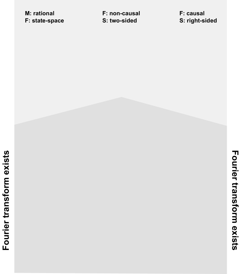
Figure 8: A block diagram identifying the algebraic structure of sets commonly used in discrete-time signal processing. Note that the module property is not captured in this diagram since it depends on the choice of algebra.

We now return to the search for an algebra. We have ruled out already above the set $\Phi({\mathbb{C}}^{\mathbb{Z}})$ as a possibility for ${\cal A}$, because multiplication of two-sided infinite series is not possible in general. Among the sets in Figure 8, the next largest candidate for ${\cal A}$ is the set of right-sided series ${\cal A}=\Phi({\mathbb{C}}^{\mathbb{N}})$. In mathematics, this is the set of formal power series, written as ${\mathbb{C}}[[z^{-1}]]$, and it is an algebra (in (22) the inner sum has only finitely many terms and is thus always well-defined). In looking for an ${\cal A}$-module ${\cal M}$ for this algebra, it is easy to verify again that the set $\Phi({\mathbb{C}}^{\mathbb{Z}})$ is not an ${\cal A}$-module (again, for $a\in{\cal A}$, $a^{\prime}\in{\cal M}$, the inner sum in (22) will have infinitely many terms; thus, the product does not exist in general). The next candidate for the corresponding ${\cal A}$-module is the regular module ${\cal M}={\cal A}$. However, there are problems with choosing for algebra of filters ${\cal A}={\mathbb{C}}[[z^{-1}]]$. First, this set contains only causal or one-sided filters. Second, the Fourier transform for the regular module ${\cal M}={\cal A}$ does not exist (note that it lies outside the dark-gray area in Figure 8).

The next largest choice for ${\cal A}$ is the space of bounded-input, bounded-output (BIBO) stable systems ${\cal A}=\Phi(\ell^{1}({\mathbb{Z}}))$. This is the set usually chosen in signal processing. As module for ${\cal A}$, we can consider again the regular module ${\cal M}={\cal A}$; in alternative, we can actually choose a larger space of signals. A well-known theorem states that $\Phi(\ell^{p}({\mathbb{Z}}))$ is a $\Phi(\ell^{1}({\mathbb{Z}}))$-module for $p\geq 1$. Thus, we could attempt to select as a module the largest of such sets ${\cal M}=\Phi(\ell^{\infty}({\mathbb{Z}}))$. The problem is that, again, as it is well-known, the Fourier transform does not exist. The choice commonly made in signal processing is ${\cal M}=\Phi(\ell^{2}({\mathbb{Z}}))$, the space of finite-energy signals. With these choices, we emphasize that for the discrete time example under consideration we chose the sets ${\cal A}$ and ${\cal M}$ to be different, i.e., the sets of filters and of signals have not only different algebraic structures (one is an algebra and the other is a module) but, as sets, they are actually different, a fact that is rarely explicitly stated in the signal processing literature. Finally, we note that because of the need for efficient implementations of filters, usually only the smaller algebra ${\mathbb{C}}(z^{-1})\!\cap\!\Phi(\ell^{1}({\mathbb{Z}}))$ of BIBO stable series that are also expansions of rational functions is considered.

In summary, with these choices ${\cal A}=\Phi(\ell^{1}({\mathbb{Z}}))$ and ${\cal M}=\Phi(\ell^{2}({\mathbb{Z}}))$, filters $h$ and signals $s$ take the form $h=H(z)=\sum_{n\in{\mathbb{Z}}}h_{n}z^{-n}$ and $s=S(z)=\sum_{n\in{\mathbb{Z}}}s_{n}z^{-n}$, respectively. The basis elements $z^{-n}$ are called delays if they are filters and impulses if they are signals.

The representation $\phi$ of ${\cal A}$ afforded by ${\cal M}$ with basis $b=(\dots,z^{-1},z^{0},z^{1},\dots)$ maps filters $h$ to a doubly infinite matrix with Toeplitz structure.

The next task is to identify the irreducible modules ${\cal M}_{\omega}$, i.e., the spectrum of ${\cal M}$. It is well-known that each

$$E_{\omega}(z)=\sum_{n\in{\mathbb{Z}}}e^{j\omega n}z^{-n},\quad\omega\in W=(-\pi,\pi],$$ (23)

is a simultaneous eigenvector for all filters $h=H(z)\in{\cal A}$, namely

$$H(z)E_{\omega}(z)=H(e^{j\omega})E_{\omega}(z),\quad\omega\in W.$$ (24)

This implies that the one-dimensional space ${\cal M}_{\omega}$ spanned by $E_{\omega}$ is an ${\cal A}$-module and irreducible (since of dimension 1). Further, (24) shows that ϕ_ω: H(z)↦H(e^jω)∈C is the irreducible representation afforded by ${\cal M}_{\omega}$ if the list of length 1 $(E_{\omega})$ is chosen as basis. Note that $\phi_{\omega}(h)=H(e^{j\omega})$ is a scalar because ${\cal M}_{\omega}$ is one-dimensional.

The corresponding Fourier transform is called the discrete-time Fourier transform (DTFT) and, since the $E_{\omega}(z)$ are orthogonal, it takes the form

$$\begin{array}[]{rrcl}\Delta:&{\cal M}&\rightarrow&\bigoplus_{\omega\in W}{\cal M}_{\omega},\\ &s=S(z)&\mapsto&(S(e^{j\omega})E_{\omega}(z))_{\omega\in W}.\end{array}$$

This matches (13), but there is one problem. The spectral components $E_{\omega}$ are not in ${\cal M}$, but only in $\Phi(\ell^{\infty}({\mathbb{Z}}))$. So, the ${\cal M}_{\omega}$ are still irreducible ${\cal A}$-modules, but not submodules of ${\cal M}$. This is one of the problems that can arise in the infinite case; in this paper we are mostly concerned with finite-dimensional modules where this problem does not occur. In the present example however, $\Delta$ still exists, and its coordinatized form (16) is the one actually called DTFT in signal processing:

$$\begin{array}[]{rrcl}\Delta:&{\cal M}&\rightarrow&\bigl{(}\bigoplus_{\omega\in W}{\mathbb{C}}\bigr{)}={\mathbb{C}}^{W},\\ &s=S(z)&\mapsto&(S(e^{j\omega}))_{\omega\in W}=\omega\mapsto S(e^{j\omega}),\end{array}$$

where $W=(-\pi,\pi]$. $\Delta(s)$ is usually viewed as function on the circle. The operation of ${\cal A}$ on ${\cal M}$, i.e., convolution, $H(z)S(z)$ becomes a set of pointwise multiplications $H(e^{j\omega})S(e^{j\omega})$ in the Fourier domain. Further, $\Delta$ can be inverted, i.e., the signal can be reconstructed from its spectrum.

Finally, the frequency response for a filter $h=H(z)\in{\cal A}$ is given by the collection of all irreducible representations evaluated at $h$: (ϕ_ω(H(z)))_ω∈W = (H(e^jω))_ω∈W = ω↦H(e^jω). Note that the frequency response of the filter $h$ is obtained in the same way as the spectrum of the signal $s$, namely by evaluating at $e^{j\omega}$, i.e., by “applying the Fourier transform” to the filter $h\in{\cal A}$ (we use double quotes since we defined the Fourier transform only for ${\cal M}$). This is due to the special structure of the algebra and module and may be misleading; in general, the spectrum (in coordinate form) consists of vectors of length $d_{\omega}$ (the dimension of ${\cal M}_{\omega}$), and the frequency response consists of $d_{\omega}\times d_{\omega}$ matrices (the representations afforded by ${\cal M}_{\omega}$). They coincide in dimensionality only for $d_{\omega}=1$.

Figure 8 suggests that many other combinations of filter algebra and signal module are possible, and this is indeed the case. For example, we can keep the signal module ${\cal M}=\Phi(\ell^{2}({\mathbb{Z}}))$ and restrict the filter algebra to a smaller algebra, e.g., to causal FIR filters ${\cal A}={\mathbb{C}}[z^{-1}]$. Choosing now this ${\cal A}$, we can reduce the signal module, for example, to the signals with finite support, ${\cal M}={\mathbb{C}}[z,z^{-1}]$, or, as another example, to the right-sided signals ${\cal M}={\cal A}$. In the algebraic framework, these would be different signal models; however, the associated spectrum and Fourier transform in these cases is essentially equivalent to the more general model considered above. We will later consider models, which have a substantially different notion of spectrum and thus also Fourier transform (as example see also Table I).

At this point we hope to have conveyed to the reader that important concepts from discrete-time signal processing are equivalent to the more general concepts from the theory of algebras and modules. This correspondence enables us to port linear signal processing to other algebras and modules. A more immediate question, however, is whether other modules and algebras are actually used in standard signal processing without being explicitly stated. This is indeed the case as hinted at in Section I, and the main motivation for developing this algebraic theory. Before we consider these models, we introduce the central concept in the algebraic theory of signal processing: the formal, algebraic definition of a signal model.

II-C Algebraic Definition of Signal Model

In the previous section we asserted that the assumptions underlying SP naturally make the filter space an algebra ${\cal A}$ and the signal space an associated ${\cal A}$-module ${\cal M}$. Conversely, if any ${\cal A}$-module ${\cal M}$ is given, filtering is automatically defined, and the well-established module theory can be applied to rigorously derive the spectrum, the Fourier transform, and the other concepts in signal processing.

However, signal processing does not commonly consider modules. In particular, signals are not viewed as elements of a module, but, in the discrete case considered here, as sequences of numbers from the base field over some index range. If the index range is fixed, e.g., $I=\{0,\dots,n-1\}$, then the corresponding set of signals, e.g., ${\mathbb{C}}^{n}$, naturally is a vector space. The question is: How do we formally associate a module to this vector space? The answer is given by the following definition of a (linear) signal model, which is the central concept in the algebraic theory of signal processing.

We consider discrete complex signals s, i.e., sequences $\text{\bf s}\in{\mathbb{C}}^{I}$ of complex numbers over some index range $I\subseteq{\mathbb{Z}}$. The set of signals is a vector space $V\leq{\mathbb{C}}^{I}$. For finite $I=\{0,\dots,n-1\}$, typically, $V={\mathbb{C}}^{\{0,\dots,n-1\}}={\mathbb{C}}^{n}$. If $I={\mathbb{N}},{\mathbb{Z}}$, we usually consider $V=\ell^{1}(I)$, $V=\ell^{2}(I)$, or $V={\mathbb{C}}^{I}$.

Definition 1 (Linear Signal Model)

Let $V\leq{\mathbb{C}}^{I}$ be a vector space of complex signals over a discrete index domain $I$. A discrete linear signal model, or just signal model, for $V$ is a triple $({\cal A},{\cal M},\Phi)$, where ${\cal A}$ is an algebra of filters, ${\cal M}$ is an ${\cal A}$-module of signals with $\dim({\cal M})=\dim(V)$, and

$$\Phi:\ V\rightarrow{\cal M}$$ (25)

is a bijective linear mapping. If ${\cal A},{\cal M}$ are clear from the context, we simply refer to $\Phi$ as the signal model.

Further, we transfer properties from ${\cal M}$ to the signal model. For example, we say the signal model is regular or finite, if ${\cal M}$ is regular or finite (-dimensional), respectively.

Note that the definition of the signal model has linearity built in (due to the operation of ${\cal A}$ on ${\cal M}$) in accordance with the algebraic theory being a theory of linear signal processing.

Remarks on signal model. Intuitively, a signal model endows the vector space $V\leq{\mathbb{C}}^{I}$ with the structure of the module ${\cal M}$ as graphically displayed in Figure 1. Via the signal model we can then identify $\text{\bf s}\in V$ with the element in the module $s=\Phi(\text{\bf s})$. As a consequence, filtering is now well-defined and we get immediate access to all module-theoretic concepts introduced in Section II-B, including spectrum, Fourier transform, and several others not yet introduced.

For example, if ${\cal M}$ is of dimension $n$ with basis $b=(b_{0},\dots,b_{n-1})$ and $\text{\bf s}\in{\mathbb{C}}^{n}$, then

$$\Phi(\text{\bf s})=s=\sum_{i=0}^{n-1}s_{i}b_{i}$$ (26)

defines a signal model for $V={\mathbb{C}}^{n}$. Conversely, if $\Phi$ is any signal model for $V$ with canonical basis $e_{i}$ ($i$th element in $e_{i}$ is 1; all other elements are 0), then the list of all $b_{i}=\Phi(e_{i})$ is a basis of ${\cal M}$ (since $\Phi$ is bijective) and thus $\Phi$ has the form in (26). In other words, the definition of signal model implicitly chooses a basis in ${\cal M}$ and $\Phi$ is dependent on this basis. In fact, we will later see examples of signal models (associated to the DCTs) that differ only in this choice of basis or $\Phi$, i.e., have the same algebra and module.

Definition 1 makes it possible to apply different signal models to the same vector of numbers. For example, we will later learn that by applying a DFT or a DCT to a vector of length $n$ one is implicitly adopting different signal models for the same finite-length vector.

From a strictly mathematical point of view, and in the algebraic definition of signal model, the bijection $\Phi$, in other words, the usual $z$-transform in signal processing, serves simply to track the basis chosen for the signal module ${\cal M}$. This basis determines the operation of the algebra on the vector space $V$.

We remark that Definition 1 of the signal model and the algebraic theory extends to the case of continuous signals. However, in this ,we will not pursue this extension and limit ourselves to discrete signals.

As an example, we show next that the $z$-transform, is the linear mapping $\Phi$ of a signal model in the sense of Definition 1. For this reason, we will refer to the linear mapping in other signal models as transforms, such as the $C$-transform or the $P$-transform that we will introduce.

Example: $z$-transform. We present the signal model for the $z$-transform. We choose as algebra A= {∑_n∈Zh_nz^-n— (…,h_-1,h_0,h_1,…)∈ℓ^1(Z)} the set of all Laurent series with $\ell^{1}$ coefficient sequences, and as module M= {∑_n∈Zs_nz^-n— (…,s_-1,s_0,s_1,…)∈ℓ^2(Z)} the set of all Laurent series with $\ell^{2}$ coefficient sequences. ${\cal M}$ is indeed an ${\cal A}$-module as we discussed in Section II-B. We complete the definition of the signal model by identifying the bijective linear mapping $\Phi$ in Definition 1. The ordinary $z$-transform will do

$$\begin{array}[]{rrcl}\Phi:&\ell^{2}({\mathbb{Z}})&\rightarrow&{\cal M}=\Phi(\ell^{2}({\mathbb{Z}})),\\ &\text{\bf s}&\mapsto&s=S(z)=\sum_{n\in{\mathbb{Z}}}s_{n}z^{-n}.\end{array}$$ (27)

In summary, $({\cal A},{\cal M},\Phi)$ is a signal model for the vector space $V=\ell^{2}({\mathbb{Z}})$. This signal model is, of course well-known and the one commonly adopted in mainstream discrete-time signal processing.

After the $z$-transform is chosen, it becomes clear how to do filtering. Namely, if $h=H(z)\in{\cal A}$ and $s=S(z)\in{\cal M}$, then the result $r=R(z)$ of filtering $s$ with $h$ is simply the product of Laurent series

$$R(z)=H(z)S(z).$$ (28)

If we work with the respective coefficient sequences, then the $n$th coefficient $r_{n}$ of $r$ follows from (28)

$$r_{n}=\sum_{i\in{\mathbb{Z}}}h_{i}s_{n-i}.$$ (29)

The signal model, the operation of ${\cal A}$ on ${\cal M}$, and the choice of transform makes clear the definition of (29) or (28). Without making explicit the algebraic structure , the origin of (29) as filtering is obscured. The problem is that in (29) filtering is defined in terms of coordinates with respect to a basis, but the basis, which explains the structure of (29), is not provided.

Signal processing books emphasize the usefulness of the $z$-transform, since common signal processing operations are conveniently expressed in the $z$-domain. In algebraic terms this means that it is more convenient to work with the explicit algebra and module rather than with the vector spaces of coefficient sequences. For this reason, we believe it is necessary to identify the signal models $({\cal A},{\cal M},\Phi)$ for all the spectral linear transforms ${\cal F}$, thus identifying ${\cal F}$ as the Fourier transform (in the algebraic sense) for ${\cal M}$. This is one of the goals achieved by the algebraic theory.

II-D Shifts, Shift-Invariance, and Commutative Algebras

So far, the only examples of algebras and modules used in signal processing that we provided are those shown in Figure 8. These are associated with infinite discrete-time signal processing. An important question is which other algebras and modules actually occur in discrete signal processing and why. It is possible to give a preliminary answer to this question by introducing and requiring the concept of shift-invariance. We start by understanding what “shift” and “shift-invariance” means in our algebraic theory by focusing first on the case where only one shift is available, i.e., on 1-D signals. Then we extend the discussion to multiple shifts.

Shift. Defining transforms and processes on groups is common in many areas. For example, in ergodic theory or in dynamical systems, a probability space is associated with a mapping, which can be a shift, that can take many different abstract forms depending on the underlying space. To be more specific, and following [Gray:88], the usual model in ergodic theory is a probability space $(\Omega,\mathcal{F},{\cal P})$ and a measurable transformation ${\cal T}$ (often called the shift). The set $\Omega$ is assumed to consist of infinite or finite duration sequences or waveforms and often assumed to be a product space of the real line (or more generally a Polish space). Measurable maps $f$ are then defined on it. Of particular interests are maps taking $\Omega$ into the real line or some subset thereof. With such a mapping $f$, then $y(t)=f({\cal T}^{t}\omega)$ for $t$ in some group gives a sequence or waveform for every $\omega\in\Omega$. The mapping $f$ produces a shift-invariant mapping from sequence (or waveform) to sequence (or waveform), which leads to a general theory for general alphabets based on when ${\cal T}$ is measure preserving (and hence the processes stationary). This general setup works for time shifts and space shifts and most signals likely to be of interest in applications.

This paper considers specific instantiations of this general theory and looks for very particular forms of the shift as they have been used in linear signal processing, or that may explain existing linear transforms or may lead to new linear transforms. To achieve this, we show that, in the algebraic theory, the shift has a particularly simple interpretation. The shift operator is a special filter, and thus is an element $x\in{\cal A}$. Further, it is common to require that every filter $h\in{\cal A}$ be expressed as a polynomial or series in the shift operator $x$. Mathematically, this means that the shift operator generates the algebra ${\cal A}$. Since a similar statement holds also for multiple shifts (discussed below):

shift(s) $=$ chosen generator(s) of ${\cal A}$

Shift-invariant algebras. A key concept in signal processing is shift-invariance. In the algebraic theory this property takes a very simple form. Namely, if $x$ is the shift operator and $h$ a filter, then $h$ is shift-invariant, if, for all signals $s$, $h(xs)=x(hs)$, which is equivalent to $hx=xh$. Requiring shift-invariance for all filters $h$ thus means

$$x\cdot h=h\cdot x,\quad\text{for all }h\in{\cal A}.$$ (30)

Since $x$ generates ${\cal A}$, ${\cal A}$ is necessarily commutative, and (30) is of course guaranteed. Conversely, if ${\cal A}$ is a commutative algebra and $x$ generates ${\cal A}$, then all filters $h\in{\cal A}$ are shift-invariant. This observation is simple but crucial, and it also holds for multiple shifts (discussed below):

shift-invariant signal model $\Leftrightarrow$  ${\cal A}$ is commutative

In particular, shift-invariance is a property of the algebra, and not of the chosen module (signal space) in a signal model. However, different choices of modules will, in general, produce different signal models as we will see later.

Which algebras are shift-invariant? We can now ask which algebras lead to shift-invariant signal models, or equivalently, which algebras ${\cal A}$ are commutative and generated by one element $x$? In fact, if ${\cal A}$ is generated by one element it is necessarily commutative; in other words, signal models with just one shift are always shift-invariant. This is different in the case of multiple shifts discussed below.

In the case of one shift, we have to identify those algebras that are generated by one element $x$. In the infinite-dimensional case, we get algebras of series in $x$ or polynomials of arbitrary degree in $x$. In the finite-dimensional case, these algebras are precisely the polynomial algebras A= C[x]/p(x), $p$ a polynomial of degree $n$. ${\mathbb{C}}[x]/p(x)$ is the set of all polynomials of degree less than $n$ with addition and multiplication modulo $p(x)$. As a vector space, ${\cal A}$ has dimension $n$.

Thus, using only shift-invariance as a requirement, we have identified one of the key players in the algebraic theory of signal processing, namely polynomial algebras. They provide the signal models for many transforms, such as the DFT, DCT, and others, and for several new transforms. This observation motivates our Section III, which develops the general theory of signal processing using polynomial algebras by specializing the general algebraic theory in Section II-B.

In the remaining discussion on shift-invariance, we consider the situation where several shifts are available and the relationship between polynomial algebras and group algebras. The reader may want to skip this part at first reading and proceed with Section II-F.

Multiple shifts. In general, if $m$-D signals are considered, $m$ shift operators $x_{1},\dots,x_{m}$ are available. These may operate along different dimensions of the signal as in the usual separable case, but can also take different forms as shown in Figure 5 for non-separable models that we derived using the present algebraic theory.

The above discussion on one shift is readily extended to multiple shifts but there are some differences. Again, the $x_{1},\dots,x_{m}$ generate ${\cal A}$ and shift-invariance becomes x_i⋅h = h⋅x_i for all   h∈A,1≤i≤k, which is equivalent to ${\cal A}$ being commutative. We can reduce this condition to

$$x_{i}\cdot x_{j}=x_{j}\cdot x_{i}.$$ (31)

In words, a signal model with $m$ shifts is shift-invariant if and only if the shifts commute in pairs.

Commutative algebras generated by $m$ elements include multivariate series (e.g., Laurent series in more than one variables).

For an exact classification, we restrict ourselves to algebras generated by $x_{1},\dots,x_{m}$ in the strict sense, i.e., those containing only multivariate polynomials, no series. In signal processing terms, this is equivalent to ${\cal A}$ containing only FIR filters. In particular, every signal model for a finite set of samples, i.e., with $\dim({\cal M})<\infty$ falls into that class.

Commutative algebras generated by $\overline{x}=(x_{1},\dots,x_{m})$ are precisely all multivariate polynomial algebras (the notation is explained in Appendix LABEL:algdefs together with the Chinese remainder theorem)

$${\cal A}={\mathbb{C}}[\overline{x}]/\langle p_{1}(\overline{x}),\dots,p_{k}(\overline{x})\rangle,$$ (32)

where $p_{i}(\overline{x})$, $1\leq i\leq k$, are polynomials in $m$ variables. In words, ${\cal A}$ is the algebra of all polynomials in $m$ variables with addition and multiplication defined modulo the $k$ polynomials $p_{i}$. Equivalently, ${\cal A}$ is the algebra of all polynomials in $m$ variables, with the restriction that the equations $p_{1}(\overline{x})=\dots=p_{k}(\overline{x})=0$ have been introduced. Mathematically, $\langle p_{1}(\overline{x}),\dots,p_{k}(\overline{x})\rangle$ is the ideal of ${\mathbb{C}}[\overline{x}]$ generated by the $p_{i}$, and the polynomial algebra is called a quotient algebra. Note that if $k=1$, i.e., $p=p_{1}$, then we write simply ${\mathbb{C}}[x]/p(x)$ instead of ${\mathbb{C}}[x]/\langle p(x)\rangle$ as we did already above.

As a remark, we observe that the polynomial algebra ${\cal A}$ can be of infinite or finite dimension. For example, for $m=1,k=0$, we get ${\mathbb{C}}[x]$, which is of infinite dimension but with countable basis. The primary example in this paper, discussed above, is the case $m=1,k=1$, i.e., ${\cal A}={\mathbb{C}}[x]/p(x)$, for some finite degree polynomial $p(x)$. This algebra is of finite dimension.

Intuitively, if $m$ is given, we need at least $k=m$ polynomials $p_{i}$ in (32) to make the dimension finite. However, conversely, choosing $k=m$ polynomials does not guarantee the polynomial algebra ${\cal A}$ to be finite-dimensional, unless $k=m=1$. Also, it is known that for $m>1$ a polynomial algebra can have arbitrary large $k$, no matter how the polynomials $p_{i}$ are chosen [Cox:97].

The 2-D signal models referred to in Figure 5, namely for spatial signals residing on a finite hexagonal or quincunx lattice, are indeed shift-invariant (and regular). The associated polynomial algebras have $k=m=2$.

Next, we briefly discuss Fourier analysis on groups to put it into the context of the algebraic theory.

Fourier analysis on groups. Let $G$ be a finite group. Take the elements of the group to be a basis for the following vector space C[G] = {∑_g∈Ga_gg∣a_g∈C}. Clearly, ${\mathbb{C}}[G]$ is a vector space, spanned by the group elements. It is also clear that we can define in a standard way multiplication of elements in ${\mathbb{C}}[G]$ by using the distributive law and the multiplication of group elements. Thus, ${\mathbb{C}}[G]$ is an algebra. Another point of view is to regard ${\mathbb{C}}[G]$ as the set of complex functions $g\mapsto a_{g}$ on the group $G$. The regular module ${\cal M}={\cal A}={\mathbb{C}}[G]$ provides a signal model in the sense of Definition 1. Namely, if $G$ has $n$ elements, we can set ${\cal A}={\cal M}={\mathbb{C}}[G]$, and

$$\begin{array}[]{rrcl}\Phi:&{\mathbb{C}}^{n}&\rightarrow&{\mathbb{C}}[G]\\ &\text{\bf s}&\mapsto&\sum_{g\in G}s_{g}g.\end{array}$$ (33)

In particular, both signals and filters are elements of the group algebra in this case. The study of the signal models $({\cal A},{\cal M},\Phi)$ in (33) is the area of Fourier analysis on finite groups (briefly discussed in the introduction), which thus becomes an instantiation of the algebraic theory of signal processing.

According to the notion of shift introduced above, we also have shift operators in a group $G$, namely the elements of the chosen generating set for $G$. Note that, unless the group is cyclic, $G$ and thus ${\mathbb{C}}[G]$ requires at least two generators, i.e., shifts. If $G$ is not commutative, then the generators will not commute in pairs, i.e., violate (31). Thus the signal model (33) is shift-variant.

An immediate question is how polynomial algebras and group algebras differ. Since polynomial algebras are always commutative, it is clear that for a non-commutative group the associated group algebra cannot be a polynomial algebra. On the other hand, it is known that every group algebra for a commutative group is a polynomial algebra with a very specific structure. Namely, a commutative group $G$ is always the direct product of cyclic groups $G=Z_{n_{1}}\times\dots\times Z_{n_{m}}$, where $Z_{n_{i}}$ is of size $n_{i}$ and is generated by $x_{i}$; thus we get

$${\mathbb{C}}[G]={\mathbb{C}}[x_{1},\dots,x_{m}]/\langle\{x_{i}^{n_{i}}-1|1\leq i\leq m\}\rangle.{\mathbb{C}}[G]={\mathbb{C}}[x_{1},\dots,x_{m}]/\langle\{x_{i}^{n_{i}}-1|1\leq i\leq m\}\rangle.$$ (34)

In the case of one variable (one-dimensional signals), $G$ is necessarily cyclic, $G=Z_{n}$, and we have

$${\mathbb{C}}[Z_{n}]={\mathbb{C}}[x]/(x^{n}-1).$$ (35)

This algebra is known to be associated to the DFT (of size $n$) as we will discuss later. Comparing (34) and (35) to general polynomial algebras in (32), it becomes clear that only very few polynomial algebras are also group algebras.

Historically, the observation that the DFT is associated to ${\mathbb{C}}[Z_{n}]$ spawned a significant effort in developing Fourier analysis for other, non-commutative groups and in deriving their fast algorithms. The observation that non-commutative groups produce shift-variant signal models may explain why these groups have to date not found many applications in signal processing.

In this paper, we investigate polynomial algebras, i.e., shift-invariant systems, and we will show that algebras other than ${\mathbb{C}}[x]/(x^{n}-1)$, and thus not related to groups, are indeed relevant in signal processing. Before we identify these algebras, we will provide a general discussion of signal processing on polynomial algebras ${\mathbb{C}}[x]/p(x)$ in Section III that specializes the algebraic concepts from Section II-B to this specific case.

Figure 9: The intersection of the set of group algebras ${\mathbb{C}}[G]$ and the set of polynomial algebras is precisely the group algebras for commutative groups $G$. In particular, for one shift (one variable, one group generator) there is only the common element ${\mathbb{C}}[Z_{n}]={\mathbb{C}}[x]/(x^{n}-1)$, which is associated to the $\operatorname{DFT}_{n}$.

II-E Visualization of a Signal Model

A given signal model can be visualized by a graph (see Appendix LABEL:algdefs, Definition LABEL:graph), which provides an intuitive understanding of the model. We will use these visualizations later.

Definition 2 (Visualization of Signal Model)

Assume that a signal model $({\cal A},{\cal M},\Phi)$ is given and Φ: s↦∑_n∈Is_nb_n, where the $b_{n}$ form a basis $b$ of ${\cal M}$. Denote the chosen shift operators, i.e., generators, of the corresponding algebra ${\cal A}$ by $x_{1},\dots,x_{n}$. Further, assume that $\phi$ is the representation of ${\cal A}$ afforded by ${\cal M}$ with basis $b$. Then each $\phi(x_{i})$ is an infinite or finite matrix (which we call shift matrix) and can be viewed as the adjacency matrix of a weighted graph ${\cal G}_{i}$. Each of these graphs has the same vertices corresponding to $b$. Thus we can join these graphs by adding the adjacency matrices of the ${\cal G}_{i}$ to obtain a graph ${\cal G}$.

We call the graph ${\cal G}$ a visualization of the signal model $({\cal A},{\cal M},\Phi)$.

Intuitively, the graph provides the topology imposed by the signal model. This will become clear by looking at the various examples shown in this paper. As a first example, we use the only signal model we have identified so far, the $z$-transform defined in (27). The chosen basis in ${\cal M}$ consists of the monomials $b=(x^{n})_{n\in{\mathbb{Z}}}$. The one available shift operator $x$ operates on $b$ as $x\cdot x^{n}=x^{n+1}$. In coordinates, this means that $\phi(x)$ is a doubly infinite matrix with ones on the lower diagonal and zeros else. The graph that has $\phi(x)$ as adjacency matrix is shown in Figure 10. The vertices are the base elements $b_{n}$, the edges show the shift.

Figure 10: Visualization of the signal model $z$-transform as a graph.

II-F Module Manipulation and Commutative Diagrams

A convenient tool when working with modules are ${\cal A}$-module homomorphisms (Definition LABEL:hommoddef in Appendix LABEL:algdefs). In particular, these mappings are linear mappings, and, in many cases considered in this paper simply base changes within one module. Since we always work with explicitly chosen bases, in the finite-dimensional case these mappings are represented by matrices. Formally, if ${\cal M}_{1},{\cal M}_{2}$ are ${\cal A}$-modules with chosen bases, and $B$ is the matrix representing the ${\cal A}$-module homomorphism w.r.t. these bases, then we write M_1⟶BM_2 Above, we already encountered an example for this arrow notation: the first row in (13) maps ${\cal M}$ to its decomposition; w.r.t. chosen bases, the mapping corresponds to the matrix form of the Fourier transform ${\cal F}$ (again, we consider only the finite-dimensional case here). If two or more mappings between modules are connected, then the associated matrices obey the following rule (the $B_{i}$ are the base change matrices): M_1⟶B1M_2 ⟶B2M_3 implies M_1⟶B2B1M_3. This identity shows that a given mapping (or matrix) from ${\cal M}_{1}$ to ${\cal M}_{3}$ can be factorized via a module ${\cal M}_{2}$. With the proper choice of inserted module, this will be a crucial tool for the derivation of fast algorithms [Pueschel:05]. In this paper, we use it for the commutative diagrams introduced below.

Another important identity is M_1⟶BM_2  implies M_2⟶B-1M_1 provided that $B$ is invertible.

The second important algebraic tool is the use of commutative diagrams, which are built from the above module mappings. A typical example looks like

(36)

The term “commutative” signifies that different paths connecting two given modules yield the same associated matrix. For example, in the above diagram, we can connect ${\cal M}_{1}$ to ${\cal M}_{4}$ in two different ways: via ${\cal M}_{2}$ or via ${\cal M}_{3}$. The diagram implies the identity B_4B_2 = B_3B_1.

III Signal Processing on Polynomial Algebras

In Section II-D we have learned that shift-invariance leads naturally to polynomial algebras ${\cal A}$ in the signal model $({\cal A},{\cal M},\Phi)$. In particular, in the case of finite 1-D signal models, these algebras are necessarily of the form ${\mathbb{C}}[x]/p(x)$. With this motivation, we investigate what it means to do signal processing using these algebras. We do this by specializing the general theory from Section II-B to ${\cal A}={\mathbb{C}}[x]/p(x)$ focusing on the regular case ${\cal M}={\cal A}$.

We start with the definition of polynomial algebras in one variable, then we investigate their spectral decomposition, their associated Fourier transforms with diagonalization properties, and formulate a general convolution theorem. The results provide the general framework for signal processing using the DFTs, DCTs, and DSTs.

III-A Polynomial Algebras in One Variable

Let $p(x)$ be a polynomial of degree $\deg(p)=n$. Then, ${\cal A}={\mathbb{C}}[x]/p(x)=\{h(x)\mid\deg(h)<n\}$, the set of residue classes modulo $p$, is an algebra with respect to the addition of polynomials, and the polynomial multiplication modulo $p$. We call ${\cal A}$ a polynomial algebra (in one variable). Polynomial algebras are always cyclic, i.e., generated by one suitable element, usually chosen to be $x$, which is then called the shift operator (see Section II-D). This means that all elements in ${\cal A}$ are obtained by repeatedly forming powers, sums, and scalar multiples from $x$. In other words, the elements are polynomials in $x$ as implicit from the definition above.

Example. As a simple instructive example, we consider $p(x)=(x-1)(x+1)=x^{2}-1$. Multiplying the two elements $x,x+1\in{\cal A}$, we get

$$x(x+1)=x^{2}+x\equiv x+1\text{ mod }(x^{2}-1)$$ (37)

by replacing $x^{2}$ with $1$. We read (37) as “$x^{2}+x$ is congruent (or equal) to $x+1$ modulo $x^{2}-1$.” Thus, we do not use “mod” as an operator, as in (x^2+x) mod (x^2-1) = x+1, but to denote equality of two polynomials modulo a third polynomial.

III-B Signal Model

We choose as vector space $V={\mathbb{C}}^{n}$, as algebra a polynomial algebra ${\cal A}={\mathbb{C}}[x]/p(x)$, $\deg(p)=n$, and as module the regular module ${\cal M}={\cal A}$. Further, we choose a basis $b=(p_{0},\dots,p_{n-1})$ of ${\cal M}$. As we show next, this provides a finite, $n$-dimensional signal model $({\cal A},{\cal M},\Phi)$ in the sense of Definition 1. Namely, if $\text{\bf s}=(s_{0},\dots,s_{n-1})^{T}\in{\mathbb{C}}^{n}$, we can define the bijective linear map $\Phi$ as

$$\Phi:\ {\mathbb{C}}^{n}\rightarrow{\cal M},\ \text{\bf s}\mapsto\sum_{0\leq\ell<n}s_{\ell}p_{\ell}.$$ (38)

Note that $\Phi$ depends on the chosen basis $b$. The basis elements $p_{i}$ are the unit impulses in ${\cal M}$, i.e., those with coordinate vector $s_{\ell}=0$ for $\ell\neq i$, and $s_{i}=1$. The impulse response of a filter $h\in{\cal A}$ for the impulse $p_{i}$ is $hp_{i}\in{\cal M}$.

The mapping $\Phi$ endows the vector space ${\mathbb{C}}^{n}$ with the structure of the ${\cal A}$-module ${\cal M}$ with basis $b$. Thus, we can now identify ${\mathbb{C}}^{n}$ and ${\cal M}$, which becomes our signal space. $\Phi$ in (38) is the equivalent of the $z$-transform for this model.

Example. Continuing our previous example, we choose the basis $b=\{1,x\}$ in ${\cal M}={\cal A}={\mathbb{C}}[x]/(x^{2}-1)$. A signal model for the vector space ${\mathbb{C}}^{2}$ is now provided by Φ: C^2→M, (s_0,s_1)↦s_0 + s_1x.

III-C Filtering

As seen before, the signal model defines filtering on the signal space ${\cal M}$ through the operation of ${\cal A}$ on ${\cal M}$. The algebra ${\cal A}$ is the space of filters and the ${\cal A}$-module ${\cal M}$ the space of signals. We mention again that even though the sets ${\cal M}$ and ${\cal A}$ are equal, their algebraic structure (i.e., the role or structure assigned to the sets) is not. For example, ${\cal A}$ operates on ${\cal M}$, not vice-versa, and filters (elements of ${\cal A}$) can be cascaded, i.e., multiplied, which signals (elements of ${\cal M}$) cannot.

We can represent filtering in either a direct way or in coordinates. Let $s=\Phi(\text{\bf s})=\sum_{0\leq\ell<n}s_{\ell}p_{\ell}\in{\cal M}$ be a signal and $h\in{\cal A}$ be a filter. Then, filtering $s$ with $h$ is simply the product

$$h\cdot s\in{\cal M},$$ (39)

i.e., the product of the polynomials $h$ and $s$ modulo $p$. Note that since the result is in ${\cal M}$, it is again a signal, as desired. Filtering, or multiplication by $h$, is a linear mapping, and so it has a matrix representation w.r.t. the basis $b$. This matrix is given by $\phi(h)$, where $\phi$ is the representation of ${\cal A}$ afforded by ${\cal M}$ with basis $b$ (see (11)). Thus, (39) becomes in coordinate form

$$\phi(h)\cdot\text{\bf s}\in{\mathbb{C}}^{n}.$$ (40)

In particular, we call the matrix $\phi(x)$ corresponding to the shift $x$ the shift matrix.

By itself, (40) does not reveal the underlying structure provided by the ${\cal A}$-module ${\cal M}$. This structure is explicit in the coordinate-free representation of filtering given in (39).

Example. In our example, let $h=h_{0}+h_{1}x\in{\cal A}={\mathbb{C}}[x]/(x^{2}-1)$ be an arbitrary filter. To compute its matrix representation $\phi(h)$ w.r.t. the basis $b=(1,x)$ of ${\cal M}$, we apply the filter to the base vectors (unit impulses) to obtain their impulse responses; the coefficient vectors of these responses are the columns of $\phi(h)$. We have $h\cdot 1=h_{0}+h_{1}x\in{\cal M}$ and $h\cdot x=h_{0}x+h_{1}x^{2}\equiv h_{1}+h_{0}x\text{ mod }(x^{2}-1)$. Thus ϕ(h) = [h0h1h1h0] and h⋅s⇔ϕ(h)⋅s. In particular, the shift matrix is given by ϕ(x) = [0 11 0 ].

III-D Visualization

The visualization of the signal model $({\cal A},{\cal M},\Phi)$ with $\Phi$ in (38) is the graph with $n$ vertices that has the shift matrix $\phi(x)$ as adjacency matrix (see Definition 2). In the general case considered in this section, this matrix has no apparent structure.

The signal models that are actually used in signal processing, however, do have structure. In particular, $\phi(x)$ is always very sparse for these models. Deriving and explaining this structure is one of the tasks that we solve in this paper.

III-E Spectrum and Fourier Transform

Unless stated otherwise, we assume that $p(x)$ is a separable polynomial, i.e., p(x) = ∏_k=0^n-1 (x - α_k), α_k≠α_ℓ, for k≠ℓ. We set $\alpha=(\alpha_{0},\dots,\alpha_{n-1})$. In words, separability means that $p$ has no zeros of multiplicity larger than 1. We will see below that this property ensures that the spectrum of ${\cal M}$ consists exclusively of one-dimensional spectral components.

The Fourier transform, or spectral decomposition, of the regular module ${\cal M}={\mathbb{C}}[x]/p(x)$ is given by the Chinese remainder theorem (CRT; stated in Theorem LABEL:crt in Appendix LABEL:algdefs) and, as filtering above, can be expressed in a direct, coordinate-free way, or, alternatively, using coordinates w.r.t. a given basis.

In a coordinate-free form, the Fourier transform is given by the mapping

$$\begin{array}[]{r@{\ }c@{\ }l}\Delta:\ {\mathbb{C}}[x]/p(x)&\rightarrow&{\mathbb{C}}[x]/(x-\alpha_{0})\oplus\dots\oplus{\mathbb{C}}[x]/(x-\alpha_{n-1}),\\ s=s(x)&\mapsto&(s(\alpha_{0}),\dots,s(\alpha_{n-1})).\end{array}$$ (41)

Each ${\cal M}_{k}={\mathbb{C}}[x]/(x-\alpha_{k})$ is of dimension 1. So the elements (vectors) of ${\mathbb{C}}[x]/(x-\alpha_{k})$ are polynomials of degree 0 or scalars $c\in{\mathbb{C}}$. Further, ${\cal M}_{k}$ is an ${\cal A}$-module, since for $h=h(x)\in{\cal A}$ and $c\in{\cal M}_{k}$, h(x)⋅c≡h(α_k)⋅c mod (x-α_k), i.e., the result is again in ${\cal M}_{k}$. Since ${\cal M}_{k}$ is of dimension 1, it is irreducible.

The scalars $s(\alpha_{k})$ in (41) are the spectral components of $s$. The mapping in (41) simultaneously projects a signal (i.e., polynomial) $s\in{\mathbb{C}}[x]/p(x)$ into the modules ${\mathbb{C}}[x]/(x-\alpha_{k})$. This projection is precisely the evaluation s(x)≡s(α_k) mod (x-α_k). The set of one-dimensional irreducible submodules ${\cal M}_{k}={\mathbb{C}}[x]/(x-\alpha_{k})$ is the spectrum of the signal space ${\cal M}$. Each submodule ${\cal M}_{k}$ is a simultaneous eigenspace to all filters (or linear systems) in ${\cal A}$. The spectrum of a signal $s\in{\cal M}$ is the vector $\Delta(s)=(s(\alpha_{0}),\dots,s(\alpha_{n-1}))$.

Example. In our running example, the Fourier transform is given by

$$\begin{array}[]{r@{\ }c@{\ }l}\Delta:\ {\mathbb{C}}[x]/(x^{2}-1)&\rightarrow&{\mathbb{C}}[x]/(x-1)\oplus{\mathbb{C}}[x]/(x+1),\\ s=s(x)&\mapsto&(s(1),s(-1)).\end{array}$$

The Fourier transform of the signal $s(x)=1+3x$ is $(4,-2)$.

III-F Frequency Response

Filtering in the regular module ${\cal M}={\mathbb{C}}[x]/p(x)$ becomes parallel filtering in the frequency domain, i.e., on the irreducible ${\cal A}$-modules ${\cal M}_{k}$. Namely, let $h\in{\cal A}$ be any filter and let $s(\alpha_{k})\in{\cal M}_{k}$ be a spectral component of a signal $s$. Then the filtering by $h$ of the signal given by this spectral component $s(\alpha_{k})$ is h(x)⋅s(α_k)≡h(α_k)s(α_k) mod (x-α_k). This shows that ${\cal M}_{k}$ affords the irreducible representation $\phi_{k}$ that maps

$$\phi_{k}:\ h=h(x)\mapsto h(\alpha_{k}).$$ (42)

The collection of the $\phi_{k}(h)$, namely $(h(\alpha_{0}),\dots,h(\alpha_{n-1}))$ is the frequency response of the filter $h$. This means that the $k$th spectral component $s(\alpha_{k})$ of a signal $s=s(x)$ is obtained in the same way as the frequency response $h(\alpha_{k})$ at $\alpha_{k}$, namely by evaluating polynomials. This is due to the simple structure of polynomial algebras; in general, this is not the case. In general, the spectral component is a $d$-dimensional vector ($d$ the dimension of the spectral component ${\cal M}_{k}$), while the frequency response of a filter $h(x)$ at this component is a $d\times d$ matrix. They have the same dimensionality only for $d=1$.

The irreducible representations $\phi_{k}$ of ${\cal A}={\mathbb{C}}[x]/p(x)$ are all different and one-dimensional, since $p$ is separable. The following lemma states that these are indeed all one-dimensional representations.

Lemma 3

Let ${\cal A}={\mathbb{C}}[x]/p(x)$, where $p$ is separable with zeros $\alpha_{0},\dots,\alpha_{n-1}$ and let $\phi:\ {\cal A}\mapsto{\mathbb{C}}$ any representation, i.e., homomorphism of algebras. Then $\phi$ is one of the $\phi_{k}$ in (42).

Proof.

Let $\phi:\ {\cal A}\mapsto{\mathbb{C}}$ be a representation. Then, because $\phi$ is a homomorphism of algebras (Definition LABEL:alghomdef in Appendix LABEL:algdefs), $p(\phi(x))=\phi(p(x))=\phi(0)=0$. Thus $\phi(x)=\alpha_{k}$ for a suitable $k$ and $\phi(h(x))=h(\phi(x))=h(\alpha_{k})$ as desired. ∎

Example. The frequency response of $h\in{\mathbb{C}}[x]/(x^{2}-1)$ is $(h(1),h(-1))$. Filtering $h\cdot s$ in ${\cal M}$ is equivalent to the point-wise product $(h(1)s(1),h(-1)s(-1))$ in the frequency domain.

III-G Fourier Transform as a Matrix

The Fourier transform $\Delta$ is a linear mapping, which can thus be expressed by a matrix ${\cal F}$ after bases are chosen. We will call this matrix also a Fourier transform for ${\cal M}$. To compute this matrix, we choose the basis $b=(p_{0},\dots,p_{n-1})$, provided by $\Phi$ in (38) for ${\cal M}$, and the basis $b_{k}=(1)$ (the list containing the polynomial $x^{0}=1$) for each summand ${\mathbb{C}}[x]/(x-\alpha_{k})$. To compute ${\cal F}$, we apply $\Delta$ to the base vectors $p_{\ell}$; the coordinate vectors of the result constitute the columns of ${\cal F}$. We compute $\Delta(p_{\ell})$ as the projection p_ℓ(x)≡p_ℓ(α_k) mod (x-α_k). Consequently, the $\ell$th-column of ${\cal F}$ is the result of applying $\Delta$ to the base vector $p_{\ell}$, namely $(p(\alpha_{0}),\dots,p(\alpha_{n-1}))^{T}$. Taken together, ${\cal F}$ has the form

$${\cal F}={\cal P}_{b,\alpha}=[p_{\ell}(\alpha_{k})]_{0\leq k,\ell<n},$$ (43)

We call ${\cal P}_{b,\alpha}$ a polynomial transform. It is uniquely determined by the signal model ${\cal A}={\cal M}={\mathbb{C}}[x]p(x)$ and $\Phi$ in (38), which fixes $b$.

This definition coincides with the notion of a polynomial transform in [Driscoll:97, Potts:98] and is related but different from the use in [Nussbaumer:79]. In [Kailath:97], polynomial transforms are called polynomial Vandermonde matrices.

Note that ${\cal P}_{b,\alpha}$ can have entries equal to zero, but, as an isomorphism (as stated by the CRT), it is necessarily invertible.

Let $s=s(x)=\sum s_{\ell}p_{\ell}(x)\in{\cal M}$ be a signal. Then, in coordinates, $\Delta$ in (41) becomes the matrix-vector product

$$\Delta(s)\Leftrightarrow{\cal P}_{b,\alpha}\cdot\text{\bf s}=(s(\alpha_{0}),\dots,s(\alpha_{n-1}))^{T}\in{\mathbb{C}}^{n}.$$ (44)

In other words, (44) computes the spectrum of s w.r.t. to the signal model $({\mathbb{C}}[x]/p(x),{\mathbb{C}}[x]/p(x),\Phi)$ with $\Phi$ defined in (38).

Like we saw with filtering before, the coordinate form (44) of the Fourier transform alone does not readily reveal the underlying signal model, i.e., the algebra and module.

The Fourier transform (in matrix form) for ${\cal M}={\mathbb{C}}[x]/p(x)$ with basis $b$ is not uniquely determined. The degree of freedom is in the choice of bases in the irreducible submodules ${\mathbb{C}}[x]/(x-\alpha_{k})$ of ${\cal M}$ in (41). If we choose generic bases $b_{k}=(a_{k})$, $a_{k}\neq 0$, in ${\mathbb{C}}[x]/(x-\alpha_{k})$, $0\leq k<n$, then the corresponding Fourier transform is given by the scaled polynomial transform diag(1/a_0,…,1/a_n-1)⋅P_b,α. We restate this in the following theorem.

Theorem 4 (Fourier Transforms)

The matrix ${\cal F}$ is a Fourier transform for the regular module ${\cal M}={\cal A}={\mathbb{C}}[x]/p(x)$ ($p$ separable), if and only if ${\cal F}$ is a scaled polynomial transform of the form

$${\cal F}=\operatorname{diag}(1/a_{0},\dots,1/a_{n-1})\cdot{\cal P}_{b,\alpha},$$ (45)

where $a_{k}\neq 0$ and $b$ is a basis for ${\cal M}$. As a consequence, any such ${\cal F}$ is invertible.

Theorem 4 is represented by the following commutative diagram (introduced in (36)):

In the top row, we have two times the module ${\mathbb{C}}[x]/p(x)$ with the same basis $b$, thus connected by the base change matrix given by the identity $\operatorname{I}_{n}$. We decompose the modules in two different ways: on the right by ${\cal P}_{b,\alpha}$, which implies the bases $(1)$ in the irreducible modules; and, on the left, by the scaled polynomial transform ${\cal F}$ given in Theorem 4, which implies the bases $(a_{k})$ in the irreducible modules. The bottom row shows the base change between the decomposed modules, which is diagonal. Connecting the top right with the bottom left corner in two different ways yields (45). In short, the diagram shows that an arbitrary Fourier transform differs from the unique polynomial transform only by a diagonal matrix.

Example. We continue our previous example $p(x)=(x-1)(x+1)$ and choose the basis $b=(1,x)$ in ${\cal M}$. The generic Fourier transform for ${\cal M}$ is given by Theorem 4 as

$$\begin{array}[]{rcl}{\cal F}&=&\operatorname{diag}(1/a_{0},1/a_{1})\cdot\begin{bmatrix}1&\phantom{-}1\\ 1&-1\end{bmatrix}\\ &=&\operatorname{diag}(1/a_{0},1/a_{1})\cdot\operatorname{DFT}_{2},\end{array}$$ (46)

where $\operatorname{DFT}_{2}=[\begin{smallmatrix}1&\phantom{-}1\\ 1&-1\end{smallmatrix}]$. In particular, $\operatorname{DFT}_{2}$ is the polynomial transform for ${\cal M}={\mathbb{C}}[x]/(x^{2}-1)$ with basis $b$.

Furthermore if s is the coordinate vector of a signal $s\in{\cal M}$ w.r.t. $b$, then DFT_2⋅s = (s(1),s(-1))^T.

III-H Diagonalization Properties and Convolution Theorems

The diagonalization property of any Fourier transform ${\cal F}$ of the regular module ${\cal M}={\mathbb{C}}[x]/p(x)$ is obtained as a special case of (21) (see also Figure 7).

Theorem 5 (Diagonalization Properties)

Let ${\cal F}$ be a Fourier transform for the regular ${\cal A}$-module ${\mathbb{C}}[x]/p(x)$ with basis $b$ and corresponding representation $\phi$ of ${\cal A}$. Then

$${\cal F}\cdot A\cdot{\cal F}^{-1}=\operatorname{diag}(a_{0},\dots,a_{n-1}),$$ (47)

if and only if $A=\phi(h)$ for a filter $h\in{\cal A}$. In this case $a_{k}=h(\alpha_{k})$, $0\leq k<n$, is the frequency response of $h$.

In particular, ${\cal F}$ diagonalizes the shift matrix $\phi(x)$. The shift operator $x$ has the frequency response $(\alpha_{0},\dots,\alpha_{n-1})$.

Proof.

Let $A=\phi(h)$. Then ${\cal F}\phi(h){\cal F}^{-1}$ is diagonal, since it is the coordinate representation of the filter $h$ in the frequency domain, which is the diagonal matrix with the frequency response on the diagonal (all blocks on the right in Figure 7 are $1\times 1$).

Conversely, the set of diagonal matrices $\operatorname{diag}(a_{0},\dots,a_{n-1})$ is an $n$-dimensional vector space. Since ${\cal F}$ is invertible, the set of all matrices $A$ diagonalized by ${\cal F}$ is also $n$-dimensional. Since ${\cal A}$ is of dimension $n$, and $\phi$ is injective, the set of all matrices $\phi(h)$ is a vector space of dimension $n$ and thus the set of all matrices diagonalized by ${\cal F}$. ∎

We also note that, using Theorem 5, we get immediately the characteristic polynomial, trace, and determinant for every matrix $\phi(h)$, since it is similar to the diagonal matrix $\operatorname{diag}(h(\alpha_{0}),\dots,h(\alpha_{n-1}))$. In particular, the characteristic polynomial of $\phi(x)$ is $p(x)$.

Example. In our example, we obtain the diagonalization property of the $\operatorname{DFT}_{2}$, namely, for $h=h_{0}+h_{1}x\in{\cal A}$, DFT_2⋅[h0h1h1h0]⋅DFT_2^-1 = diag(h(1), h(-1)). The characteristic polynomial of the shift matrix $\phi(x)=\phi(0+1\cdot x)=[\begin{smallmatrix}0&1\\ 1&0\end{smallmatrix}]$ is $p(x)=x^{2}-1$.

Theorem 5 provides the essential step to obtaining a convolution theorem in ${\cal M}$, i.e., a way to perform filtering in the spectral domain. Namely, starting from the coordinate form (40) of filtering, and using (47), we get for all $\text{\bf a}\in{\mathbb{C}}^{n}$

$$\begin{array}[]{rcl}\phi(h)\cdot\text{\bf s}&=&{\cal F}^{-1}{\cal F}\phi(h){\cal F}^{-1}{\cal F}\cdot\text{\bf s}\\ &=&{\cal F}^{-1}\operatorname{diag}(h(\alpha_{0}),\dots,h(\alpha_{n-1})){\cal F}\cdot\text{\bf s},\end{array}$$ (48)

which again shows that multiplication by $\phi(h)$ is the same as multiplying by $\operatorname{diag}(h(\alpha_{0}),\dots,h(\alpha_{n-1}))$, the frequency response, in the spectral domain. This is illustrated in the following commutative diagram:

Filtering in the signal space (top row) is equivalent to pointwise multiplication in the spectral domain (bottom row). Connecting the top left with the top right corner in two different ways yields (48).

Next, we derive the general form of the convolution theorem. Since, as said above, the frequency response is obtained in the same way as the spectrum (evaluation of polynomials at the $\alpha_{k}$), we can also compute it using a Fourier transform, even though we did not introduce a Fourier transform for elements in the algebra.

Namely, we choose a basis $b^{\prime}$ in ${\cal A}$ and let h be the coordinate vector of $h$ w.r.t. $b^{\prime}$. Then we choose a second arbitrary Fourier transform ${\cal F}^{\prime}=D\cdot{\cal P}_{b^{\prime},\alpha}$, where $D$ is diagonal. Using (44), P_b’,α⋅h = D^-1⋅(h(α_0),…,h(α_n-1))^T. Combining this equation with (48) yields the following theorem.

Theorem 6 (Convolution Theorem)

Using previous notation, let ${\cal M}$ have basis $b$ and ${\cal A}={\cal M}$ have basis $b^{\prime}$. Let $s\in{\cal M}$ and $h\in{\cal A}$. Further, let ${\cal F}$ and ${\cal F}^{\prime}=D\cdot{\cal P}_{b^{\prime},\alpha}$ be any Fourier transforms of ${\cal M}$ w.r.t. the bases $b$ and $b^{\prime}$, respectively. Then ϕ(h)⋅s = (DF)^-1⋅((F’⋅h)⊙(F⋅s)), where $\odot$ denotes the pointwise product of vectors.

Example. We illustrate Theorem 6 using our example ${\mathbb{C}}[x]/(x^{2}-1)$ with basis $(1,x)$, choosing ${\cal F}^{\prime}={\cal F}=\operatorname{DFT}_{2}$. We get the well-known convolution theorem for the DFT (of size 2): [h0h1h1h0]⋅s = DFT_2^-1⋅(DFT