Low-rank matrix factorization with attributes

Abstract

We develop a new collaborative filtering (CF) method that combines both previously known users’ preferences, i.e. standard CF, as well as product/user attributes, i.e. classical function approximation, to predict a given user’s interest in a particular product. Our method is a generalized low rank matrix completion problem, where we learn a function whose inputs are pairs of vectors – the standard low rank matrix completion problem being a special case where the inputs to the function are the row and column indices of the matrix. We solve this generalized matrix completion problem using tensor product kernels for which we also formally generalize standard kernel properties. Benchmark experiments on movie ratings show the advantages of our generalized matrix completion method over the standard matrix completion one with no information about movies or people, as well as over standard multi-task or single task learning methods.

1 Introduction

Collaborative Filtering (CF) refers to the task of predicting preferences of a given user based on their previously known preferences as well as the preferences of other users. In a book recommender system, for example, one would like to suggest new books to a customer based on what he and others have recently read or purchased. This can be formulated as the problem of filling a matrix with customers as rows, objects (e.g., books) as columns, and missing entries corresponding to preferences that one would like to infer. In the simplest case, a preference could be a binary variable (thumbs up/down), or perhaps even a more quantitative assessment (scale of 1 to 5).

Standard CF assumes that nothing is known about the users or the objects apart from the preferences expressed so far. In such a setting the most common assumption is that preferences can be decomposed into a small number of factors, both for users and objects, resulting in the search for a low-rank matrix which approximates the partially observed matrix of preferences. This problem is usually a difficult non-convex problem for which only heuristic algorithms exist [14]. Alternatively convex formulations have been obtained by relaxing the rank constraint by constraining the trace norm of the matrix [15].

In many practical applications of CF, however, a description of the users and/or the objects through attributes (e.g., gender, age) or measures of similarity is available. In that case it is tempting to take advantage of both known preferences and descriptions to model the preferences of users. An important benefit of such a framework over pure CF is that it potentially allows the prediction of preferences for new users and/or new objects. Seen as learning a preference function from examples, this problem can be solved by virtually any algorithm for supervised classification or regression taking as input a pair (user, object). If we suppose for example that a positive definite kernel between pairs can be deduced from the description of the users and object, then learning algorithms like support vector machines or kernel ridge regression can be applied. These algorithms minimize an empirical risk over a ball of the reproducing kernel Hilbert space (RKHS) defined by the pairwise kernel.

Both the rank constraint and the RKHS norm restriction act as regularization based on prior hypothesis about the nature of the preferences to be inferred. The rank constraint is based on the hypothesis that preferences can be modelled by a limited number or factors to describe users and objects. The RKHS norm constraint assumes that preferences vary smoothly between similar users and similar objects, where the similarity is assessed in terms of the kernel for pairs.

The main contribution of this work is to propose a framework which combines both regularizations on the one hand, and which interpolates between the pure CF approach and the pure attribute-based approaches on the other hand. In particular, the framework encompasses low-rank matrix factorization for collaborative filtering, multi-task learning, and classical regression/classification over product spaces. We show on a benchmark experiment of movie recommendations that the resulting algorithm can lead to significant improvements over other state-of-the-art methods.

2 Kernels and tensor product spaces

In this section, we review the classical theory of tensor product reproducing kernel Hilbert spaces, providing a natural generalization of finite-dimensional matrices for functions of two variables. The general setup is as follows. We consider the general problem of estimating a function $f:\mathcal{X}\times\mathcal{Y}\rightarrow\mathbb{R}$ given a finite set of observations in $\mathcal{X}\times\mathcal{Y}\times\mathbb{R}$. We assume that both spaces $\mathcal{X}$ and $\mathcal{Y}$ are endowed with positive semi-definite kernels, respectively $k:\mathcal{X}\times\mathcal{X}\rightarrow\mathbb{R}$ and $g:\mathcal{Y}\times\mathcal{Y}\rightarrow\mathbb{R}$, and denote by $\mathcal{K}$ and $\mathcal{G}$ the corresponding RKHS. A typical application of this setting is where $\mathbf{x}\in\mathcal{X}$ is a person, $\mathbf{y}\in\mathcal{Y}$ is a movie, kernels $k$ and $g$ represent similarities between persons and movies, respectively, and $f\left(\mathbf{x},\mathbf{y}\right)$ represents a person’s $\mathbf{x}$ rating of a movie $\mathbf{y}$. We note that if $\mathcal{X}$ and $\mathcal{Y}$ are finite sets, then $f$ is simply a matrix of size $\left|\,\mathcal{X}\,\right|\times\left|\,\mathcal{Y}\,\right|$.

2.1 Tensor product kernels and RKHS

We denote by $k_{\otimes}:\left(\mathcal{X}\times\mathcal{Y}\right)\times\left(\mathcal{X}\times\mathcal{Y}\right)\rightarrow\mathbb{R}$ the tensor product kernel, known to be a positive definite kernel [4, p.70]:

$$k_{\otimes}\left(\left(\mathbf{x}_{1},\mathbf{y}_{1}\right),\left(\mathbf{x}_{2},\mathbf{y}_{2}\right)\right)=k\left(\mathbf{x}_{1},\mathbf{x}_{2}\right)g\left(\mathbf{y}_{1},\mathbf{y}_{2}\right)\;,$$ (1)

and by $\mathcal{H}_{\otimes}$ the associated RKHS. A classical result of Aronszajn [2] states that $\mathcal{H}_{\otimes}$ is the tensor product of the two spaces $\mathcal{K}$ and $\mathcal{G}$ (denoted $\mathcal{K}\otimes\mathcal{G}$), i.e., $\mathcal{H}_{\otimes}$ is the completion of all functions $f:\mathcal{X}\times\mathcal{Y}\to\mathbb{R}$, which can be finitely decomposed as $f(x,y)=\sum_{k=1}^{p}u_{k}(x)v_{k}(y)$, where $u_{k}\in\mathcal{K}$ and $v_{k}\in\mathcal{G}$, $k=1,\dots,p$. An atomic term defined as $f(x,y)=u(x)v(y)$, with $u\in\mathcal{K}$ and $v\in\mathcal{G}$, is usually denoted $f=u\otimes v$. The space $\mathcal{H}_{\otimes}$ is equipped with a norm such that $\|u\otimes v\|_{\otimes}=\|u\|_{\mathcal{K}}\times\|v\|_{\mathcal{G}}$, and thus $\|\sum_{k}u_{k}\otimes v_{k}\|^{2}=\sum_{k,l}\langle u_{k},u_{l}\rangle_{\mathcal{K}}\langle v_{k},v_{l}\rangle_{\mathcal{G}}$.

2.2 Rank

An element of $\mathcal{H}_{\otimes}$ can always be decomposed as a possibly infinite sum of atomic terms of the form $u(x)v(y)$ where $u\in\mathcal{K}$ and $v\in\mathcal{G}$. We define the rank $\text{rank}(f)\in\mathbb{N}\cup\{\infty\}$ of an element $f$ of $\mathcal{H}_{\otimes}$ as the minimal number of atomic terms in any decomposition of $f$, i.e, $\text{rank}(f)$ is the smallest integer $p$ such that $f$ can be expanded as:

$$f\left(\mathbf{x},\mathbf{y}\right)=\sum_{1=1}^{p}u_{i}\left(\mathbf{x}\right)v_{i}\left(\mathbf{y}\right)\;,$$

for some functions $u_{1},\ldots,u_{p}\in\mathcal{K}$ and $v_{1},\ldots,v_{p}\in\mathcal{G}$, if such an integer $p$ does exist (otherwise, the rank is infinite).

When the two RKHS are spaces of linear functions on an Euclidean space, then the tensor product can be identified to the space of bilinear forms on the product of the two Euclidean spaces, and the notion of rank coincides with the usual notion of rank for matrices. We note that an alternative characterization of $\text{rank}(f)$ is the supremum of the ranks of the matrices $M$ defined by $M_{i,j}=f\left(\mathbf{x}_{i},\mathbf{y}_{j}\right)$ over the choices of finite sets $\mathbf{x}_{1},\ldots,\mathbf{x}_{m}\in\mathcal{X}$ and $\mathbf{y}_{1},\ldots,\mathbf{y}_{p}\in\mathcal{Y}$ (see technical annex for a proof).

2.3 Trace norm

Given a rectangular matrix $M$, the rank is not an easy function to optimize or constrain, since it is neither convex nor continuous. Following the 1-norm approximation to the 0-norm, the trace norm has emerged has an efficient convex approximation of the rank [8, 15]. The trace norm $\|M\|_{\ast}$ is defined as the sum of the singular values. This definition is not easy to extend to functional tensor product spaces because it involves eigen-decompositions. Rather, we use the equivalent formulation

$$\|M\|_{\ast}=\inf_{M=UV}\frac{1}{2}(\|U\|_{F}^{2}+\|V\|_{F}^{2})$$

where $\|U\|_{F}^{2}=\mathop{\rm tr}UU^{\top}$ is the squared Frobenius norm.

We thus extend the notion of trace norm as

$$\|f\|_{\ast}=\inf_{f=\sum_{k=1}^{\infty}u_{k}\otimes v_{k}}\frac{1}{2}\sum_{k=1}^{\infty}(\|u_{k}\|_{\mathcal{K}}^{2}+\|v_{k}\|_{\mathcal{G}}^{2})$$

Lemma 1

This is a norm, equal to the sum of singular values when the two RKHS are spaces of linear functions on an Euclidean space.

The main attractiveness of the trace norm is its convexity [8, 15]. However, the trace norm does not readily yield a representer theorem, and as shown in Section 3.3, it is more practical to penalize the trace norm of the matrix of estimates.

3 Representer theorems

In this section we explicitly state and prove representer theorems in tensor product spaces when a functional is minimized with rank constraints. These theorems underlie the algorithms proposed in the next section.

In a collaborative filtering task, the data usually have a matrix form, i.e., many $\mathbf{x}$’s (resp. $\mathbf{y}$’s) are identical. We let $\mathbf{x}_{1},\dots,\mathbf{x}_{n_{\mathcal{X}}}$ denote the $n_{\mathcal{X}}$ distinct values of elements of $\mathcal{X}$ in the training data, and, respectively, $\mathbf{y}_{1},\dots,\mathbf{y}_{n_{\mathcal{Y}}}$ denote the $n_{\mathcal{Y}}$ distinct values of elements of $\mathcal{Y}$. We assume that we have observations of only a subset of $\{1,\dots,n_{\mathcal{X}}\}\times\{1,\dots,n_{\mathcal{Y}}\}$. We thus denote $i(u)$ and $j(u)$ the indices of the $u$-th observation and $z_{u}$ the observed target.

3.1 Classical representer theorem in the tensor product RKHS

Given a loss function $\ell:\mathbb{R}\times\mathbb{R}\rightarrow\mathbb{R}$, for example the square loss function $\ell(z,z^{\prime})=(z-z^{\prime})^{2}$, a first classical approach to learn dependencies between the pair $\left(\mathbf{x},\mathbf{y}\right)$ and the variable $z$ is to consider it as a supervised learning problem over the product space $\mathcal{X}\times\mathcal{Y}$, and for example to search for a function in the RKHS of the product kernel which solves the following problem:

$$\min_{f\in\mathcal{H}_{\otimes}}\left\{\frac{1}{n}\sum_{u=1}^{n}\ell\left(f\left(\mathbf{x}_{i(u)},\mathbf{y}_{j(u)}\right),z_{u}\right)+\lambda\Arrowvert\,f\,\Arrowvert_{\otimes}^{2}\right\}\;.$$ (2)

By the representer theorem [9] the solution of (2) has an expansion of the form:

$$f\left(\mathbf{x},\mathbf{y}\right)=\sum_{u=1}^{n}\alpha_{u}k_{\otimes}\left(\left(\mathbf{x}_{i(u)},\mathbf{y}_{i(u)}\right),\left(\mathbf{x},\mathbf{y}\right)\right)=\sum_{u=1}^{n}\alpha_{u}k\left(\mathbf{x}_{i(u)},\mathbf{x}\right)g\left(\mathbf{y}_{j(u)},\mathbf{y}\right)\;,$$

for some vector $\left(\alpha_{1},\ldots,\alpha_{n}\right)\in\mathbb{R}^{n}$. Note that the number of parameters $\alpha$ is the number of observed values. For many loss functions the problem (2) boils down to classical machine learning algorithms such as support vector machines, kernel logistic regression or kernel ridge regression, which can be solved by usual implementations with the product kernel (1).

3.2 Representer theorem with rank constraint

In order to take advantage of the possible representation of our predictor as a sum of a small number of factors, we propose to consider the following generalization of (2):

$$\min_{f\in\mathcal{H}_{\otimes},\text{ rank}(f)\leqslant p}\left\{\frac{1}{n}\sum_{u=1}^{n}\ell\left(f\left(\mathbf{x}_{i(u)},\mathbf{y}_{j(u)}\right),z_{u}\right)+\lambda\Arrowvert\,f\,\Arrowvert_{\otimes}^{2}\right\}\;.$$ (3)

As the following proposition shows, the solution of this constrained minimization problem can also be reduced to a finite-dimensional optimization problem (see a proof in the technical annex):

Proposition 1

The optimal solution of (3) can be written as $f=\sum_{i=1}^{p}u_{i}\otimes v_{i}$, where

$$u_{i}\left(\mathbf{x}\right)=\sum_{l=1}^{n_{\mathcal{X}}}\alpha_{li}k\left({\mathbf{x}}_{l},\mathbf{x}\right)\quad\text{ and }\quad v_{i}\left(\mathbf{y}\right)=\sum_{l=1}^{n_{\mathcal{Y}}}\beta_{li}g\left({\mathbf{y}}_{l},\mathbf{y}\right),\quad i=1,\ldots,p,$$ (4)

where $\alpha\in\mathbb{R}^{n_{\mathcal{X}}\times p}$ and $\beta\in\mathbb{R}^{n_{\mathcal{Y}}\times p}$

This proposition is a crucial contribution of this paper as it allows to learn the function $f$, by learning the coefficients $\alpha$ and $\beta$: denoting by $\alpha_{k}$ the $k$-th column of $\alpha$ (similarly for $\beta$), we obtain from Proposition 1 that an equivalent formulation of (3) is:

$$\min_{\alpha\in\mathbb{R}^{n_{\mathcal{X}}\times p},\beta\in\mathbb{R}^{n_{\mathcal{Y}}\times p}}\left\{\frac{1}{n}\sum_{u=1}^{n}\ell\left(\sum_{k=1}^{p}(K\alpha_{k})_{i(u)}(G\beta_{k})_{j(u)},z_{u}\right)+\lambda\sum_{i=1}^{p}\sum_{j=1}^{p}\alpha_{i}^{\top}K\alpha_{j}\beta_{i}^{\top}G\beta_{j}\right\}$$ (5)

where $K$ is the $n_{\mathcal{X}}\times n_{\mathcal{X}}$ kernel matrix for the elements of $\mathcal{X}$ (similarly for $G$). In order to link with the trace norm formulation in the next section, if we denote $\gamma=\sum_{k=1}^{p}\alpha_{k}\beta_{k}^{\top}$, we note that the $n_{\mathcal{X}}\times n_{\mathcal{Y}}$ matrix of predicted values is equal to $F=K\gamma G$ resulting in the following optimization problem:

$$\min_{\gamma=\sum_{k}\alpha_{k}\beta_{k}^{\top}}\left\{\frac{1}{n}\sum_{u=1}^{n}\ell\left((K\gamma G)_{i(u),j(u)},z_{u}\right)\right\}+\lambda\mathop{\rm tr}\gamma^{\top}K\gamma G\;.$$ (6)

3.3 Representer theorems and trace norm

The trace norm does not readily lead to a representer theorem and a finite dimensional optimization problem. It is thus preferable to penalize the trace norm of the predicted values $F_{ij}=f(\mathbf{x}_{i},\mathbf{y}_{j})$, and minimize

$$\min_{f\in\mathcal{H}_{\otimes}}\left\{\frac{1}{n}\sum_{u=1}^{n}\ell\left(f\left(\mathbf{x}_{i(u)},\mathbf{y}_{j(u)}\right),z_{u}\right)+\mu\|(f(\mathbf{x}_{i},\mathbf{y}_{j}))\|_{\ast}+\lambda\Arrowvert\,f\,\Arrowvert_{\otimes}^{2}\right\}\;.$$ (7)

We have the following representer theorem (whose proof is postponed to the technical annex) for the problem (7):

Proposition 2

The optimal solution of (7) can be written in the form $f(x,y)=\sum_{i=1}^{n_{\mathcal{X}}}\sum_{j=1}^{n_{\mathcal{Y}}}\gamma_{ij}k(x,x_{i})k(y,y_{j})$, where $\gamma\in\mathbb{R}^{n_{\mathcal{X}}\times n_{\mathcal{Y}}}$.

The optimization problem can thus be rewritten as:

$$\min_{\gamma\in\mathbb{R}^{n_{\mathcal{X}}\times n_{\mathcal{Y}}}}\left\{\frac{1}{n}\sum_{u=1}^{n}\ell\left((K\gamma G)_{i(u),j(u)},z_{u}\right)+\mu\|K\gamma G\|_{\ast}+\lambda\mathop{\rm tr}\gamma^{\top}K\gamma G\right\}$$ (8)

Note that in contrast to the finite representation without any constraint on the rank or the trace norm (where the number of parameters is the number of observed values), the number of parameters is the total number of elements in the matrix, and this method, though convex, is thus of higher computational complexity.

3.4 Reformulation in terms of Kronecker products

Kronecker products

Given a matrix $B\in\mathbb{R}^{m\times n}$ and a matrix $C\in\mathbb{R}^{p\times q}$, the Kronecker product $A=B\otimes C$ is a matrix in $\mathbb{R}^{mp\times nq}$ defined by blocks of size $p\times q$ where the block $(i,j)$ is $b_{ij}C$.

The most important properties are the following (where it is assumed that all matrix operations are well-defined): $(A\otimes B)(C\otimes D)=AC\otimes BD$, $(A\otimes B)^{-1}=A^{-1}\otimes B^{-1}$, $(A\otimes B)^{\top}=A^{\top}\otimes B^{\top}$, and if $Y=CXB^{\top}\Leftrightarrow\text{vec}(Y)=(B\otimes C)\text{vec}(X)$ where $\text{vec}(X)$ is the stack of columns of $X$.

Reformulation

We have $M=K\gamma G$, and thus $\text{vec}(M)$ is the vector of predicted values for all pairs $(x_{i},y_{j})$ and is equal to $\text{vec}(M)=(K\otimes G)\text{vec}(\gamma)$. The matrix $K\otimes G$ is the kernel matrix associated with all pairs, for the kernel $k_{\otimes}$. The results in this section does not provide additional representational power beyond the kernel $k_{\otimes}$, but present additional regularization frameworks for tensor product spaces. In the next section, we tackle the representational part of our contribution and show how the kernels $k$ and $g$ can be tailored to the task of matrix completion.

4 Kernels for matrix completion with attributes

The three formulations (2), (3) and (7) differ in the way they handle regularization. They all require a choice of kernel over $\mathcal{X}$ and $\mathcal{Y}$ to define the RKHS norm in $\mathcal{H}_{\otimes}$, which we discuss in this section. The main theme of this section is the distinction between kernels linked to the attributes and the kernel linked to the identities of each different $\mathbf{x}$ and $\mathbf{y}$ (referred to as Dirac kernels).

Dirac kernels

In the standard collaborative filtering framework, where no attribute over $\mathbf{x}$ or $\mathbf{y}$ is available, a natural kernel over $\mathcal{X}$ and $\mathcal{Y}$ is the Dirac kernel ($k_{Dirac}(\mathbf{x},\mathbf{x}^{\prime})=1$ if $\mathbf{x}=\mathbf{x}^{\prime}$, $0$ otherwise). If both $k$ and $g$ are Dirac kernels, then $k_{\otimes}$ is also a Dirac kernel by (1) and the classical approach (2) is irrelevant in that case (the function $f$ being equal to $0$ on unseen examples). The low-rank constraint added in (3) results in a relevant problem: in fact for $\lambda=0^{+}$ we exactly recover the classical low-rank matrix factorization problem.

Attribute kernels

When attributes are available, they can be used to define kernels which we denote $k_{Attributes}$ below. When both $k$ and $g$ are kernels derived from attributes, then (2) boils down to classical regression or classification over pairs. Problem (3) provides an alternative problem, where the rank of the function is constrained.

Multi-task learning

Suppose now that attributes are available only for objects in $\mathcal{X}$, and not for $\mathcal{Y}$. It is then possible to take $k=k_{Attribute}$ and $g=k_{Dirac}$. In that case the optimization problem (2) boils down to solving a classical classification or regression problem for each value $y_{i}$ independently. Adding the rank constraint in (3) removes the independence among tasks by enforcing a decomposition of the tasks into a limited number of factors, which leads to an algorithm for multitask learning, based on a low-rank representation of the predictor function. This approach is to be contrasted with the framework of [7], which is equivalent to $\mathcal{X}$ finite of cardinality $p$, and $k\left(\mathbf{x},\mathbf{x}^{\prime}\right)=1-\lambda+\lambda pk_{Dirac}$. Our framework focuses on a low rank representation for the predictor of each task, while the framework of [7] focuses on a set of predictor for each task that has small variance. An extension of this multi-task learning framework, leading to similar penalizations by trace norms, was independently derived by Argyriou et al. [1].

General formulation

Supposing now that attributes are available on both $\mathcal{X}$ and $\mathcal{Y}$, let us consider the following interpolated kernels:

$$\begin{cases}k=\eta k_{Attribute}^{x}+(1-\eta)k_{Dirac}^{x},\\ g=\zeta k_{Attribute}^{y}+(1-\zeta)k_{Dirac}^{y},\\ \end{cases}$$

where $0\leq\eta\leq 1$ and $0\leq\zeta\leq 1$. The resulting product kernel is a sum of four terms:

$$k_{\otimes}=\eta\zeta k_{Attribute}^{x}k_{Attribute}^{y}+\eta(1-\zeta)k_{Attribute}^{x}k_{Dirac}^{y}+$$

$$+(1-\eta)\zeta k_{Dirac}^{x}k_{Attribute}^{y}+(1-\eta)(1-\zeta)k_{Dirac}^{x}k_{Dirac}^{y}.$$

By varying $\eta$ and $\zeta$ this kernel provides an interpolation between collaborative filtering ($\eta=\zeta=0$), classical attribute-based regression on pairs ($\eta=\zeta=1$), and multi-task learning ($\eta=0$ and $\zeta=1$, or $\eta=1$ and $\zeta=0$).

In terms of kernel matrices on the set of all pairs, if we denote $K_{Att}$ the kernel matrix associated with the attributes associated with $\mathcal{X}$, and $G_{Att}$ the kernel matrix associated with the attributes associated with $\mathcal{Y}$, this is equivalent to using the matrix $(\eta K_{Att}+(1-\eta)I)\otimes(\zeta G_{Att}+(1-\zeta)I)=\eta\zeta K_{Att}\otimes G_{Att}+\eta(1-\zeta)K_{Att}\otimes I+(1-\eta)\zeta I\otimes G_{Att}+(1-\eta)(1-\zeta)I\otimes I$, which is the sum of four positive kernel matrices. The first one is simply the kernel matrix for the tensor product space, while the last one is proportional to identity and usually appears in kernel methods as the numerical effect of regularization [13]. The two additional matrices makes the learning across rows and columns possible.

Generalization to new points

One the usual drawbacks of collaborative filtering is the impossibility to generalize to unseen data points (i.e., a new movie or a new person in the context of movie recommendation). When attributes are used, a prediction based on those can be made, and thus using attributes has an added benefit beyond better performance on matrix completion tasks.

5 Algorithms

In this section, we describe the algorithms used for the optimization formulation in (5) and (8). We also show that recent developments in multiple kernel learning can be applied to both setting (enforced rank constraint or trace norm).

5.1 Fixed rank

The function $(\alpha,\beta)\mapsto\frac{1}{n}\sum_{u=1}^{n}\ell\left(\sum_{k=1}^{p}(K\alpha_{k})_{i(u)}(L\beta_{k})_{j(u)},z_{u}\right)+\lambda\sum_{i=1}^{p}\sum_{j=1}^{p}\alpha_{i}^{\top}K\alpha_{j}\beta_{i}^{\top}G\beta_{j}$ is convex in each argument separately but is not jointly convex. There are thus two natural optimization algorithms: (1) alternate convex minimization with respect to $\alpha$ and $\beta$, and (2) direct joint minimization using Quasi-Newton iterative methods [5](in simulations we have used the latter scheme).

As in [12], the fixed rank formulation, although not convex, has the advantage of being parameterized by low-rank matrices and is thus of much lower complexity than the convex formulation that we know present. We present experimental results in the next section using only this fixed rank formulation.

5.2 Convex formulation

If the loss $\ell$ is convex, then the function $\gamma\mapsto\frac{1}{n}\sum_{u=1}^{n}\ell\left((K\gamma G)_{i(u),j(u)},z_{u}\right)+\mu\|K\gamma G\|_{\ast}+\lambda\mathop{\rm tr}\gamma^{\top}K\gamma G$ is a convex function. However, even when the loss is differentiable, the trace norm is non differentiable, which makes iterative descent methods such as Newton-Raphson non applicable [6].

For specific losses which are SDP-representable, i.e., which can represented by a semi-definite program, such as the square loss or the hinge loss, the minimization of this function can be cast as semi-definite program (SDP) [6]. For differentiable losses which are not SDP-representable, such as the logistic loss, an efficient algorithm is to modify the trace norm to make it differentiable (see e.g [12]). For example, instead of penalizing the sum of singular values $\lambda_{i}$, one may penalize the sum of $\sqrt{\lambda_{i}+\varepsilon^{2}}$, which leads to a twice differentiable function [10].

5.3 Learning the kernels

In this section, we show that the rank constraint and the trace norm constraint can also be used in the multiple kernel learning framework [3, 11]. We can indeed show that if the loss $\ell$ is convex, then, as a function of the kernel matrices, the optimal values of the optimization problems (5) and (8) are convex functions, and thus the kernel can be learned efficiently by minimizing those functions. We do not use this method in our experiments, however, we only include this for completeness.

Proposition 3

Given $\beta_{1},\dots,\beta_{p}$, the following function is convex in $K$:

$$K\mapsto\min_{\alpha}\left\{\frac{1}{n}\sum_{u=1}^{n}\ell\left(\sum_{k=1}^{p}(K\alpha_{k})_{i(u)}(L\beta_{k})_{j(u)},z_{u}\right)+\lambda\sum_{i=1}^{p}\sum_{j=1}^{p}\alpha_{i}^{\top}K\alpha_{j}\beta_{i}^{\top}G\beta_{j}\right\}\;.$$

The following function only depends on the Kronecker product $K\otimes G$ and is a convex function of $K\otimes G$.

$$(K,G)\mapsto\min_{\gamma\in\mathbb{R}^{n_{\mathcal{X}}\times n_{\mathcal{Y}}}}\left\{\frac{1}{n}\sum_{u=1}^{n}\ell\left((K\gamma G)_{i(u),j(u)},z_{u}\right)+\mu\|K\gamma G\|_{\ast}+\lambda\mathop{\rm tr}\gamma^{\top}K\gamma G\right\}\;.$$

This proposition (whose proof is in the technical annex) shows that in the case of the rank constraint (5), if we parameterize $K$ as $K=\sum_{j}\eta_{j}K_{j}$, the weights $\eta$ and $\alpha$ can be learned simultaneously [3, 11]. In particular, the optimal weighting between attributes and the Dirac Kernel can be learned directly from data. Note that a similar proposition holds when the role of $x$ and $y$ are exchanged; when alternate minimization is used to minimize the objective function, the kernels can be learned at each step. In the case of the trace norm constraint (8) it shows that we can learn a linear combination of basis kernels, either the 4 kernels presented earlier obtained from Dirac’s and attributes, or more general combinations. We leave this avenue open for future research.

6 Experiments

We tested the method on the well-known MovieLens 100k dataset from the GroupLens Research Group at the University of Minnesota. This dataset consists of ratings of 1682 movies by 943 users. The ratings consisted of a score from the range 1 to 5, where 5 is the highest ranking. Each user rated some subset of the movies, with a minimum of 20 ratings per user, and the total number of ratings available is exactly 100,000, averaging about 105 per user. To speed up the computation, we used a random subsample of 800 movies and 400 users, for a total of 20541 ratings. We divided this set into 18606 training ratings and 1935 for testing. This dataset was rather appropriate as it included attribute information for both the movies and the users. Each movie was labelled with at least one among $19$ genres (e.g., action or adventure), while users’ attributes age, gender, and an occupation among a list of $21$ occupations (e.g., administrator or artist).

We performed experiments using the rank constraint described in 3, and we used the more standard approach of cross validation to choose kernel parameters. Thus, our method requires selection of four parameters: the rank $d$ of the estimation matrix; the regularization parameter $\lambda$; and the values $\eta,\zeta\in[0,1]$, the tradeoff between the Dirac kernel and Attribute kernel, for the users and movies respectively. The parameters $\lambda$ and $d$ both act as regularization parameters and we choose them using cross validation. The values $\eta,\zeta$ were chosen out of $\{0,0.15,0.5,0.85,1\}$, the rank $d$ ranged over $\{50,80,130,200\}$, and $\lambda$ was chosen from $\{25,5,1,0.2,0.04\}\times 10^{-6}$.

In Table 1, we show the performance for various choices or rank $d$ and for various values of $\eta$ and $\zeta$, after selecting $\lambda$ in each case using cross-validation. We also show in bold the performance for the parameters selected using cross-validation. Notice that, performance is consistently worse when $\eta$ and $\zeta$ are chosen at the corners when compared with values at the interior of $[0,1]\times[0,1]$. We observed this to be true, in fact, not only when $d$ and $\lambda$ are chosen by cross-validation, but for every choice of $d$ and $\lambda$. Figure 1 shows the test mean squared error for $d$ and $\lambda$ selected at each point using cross validation (Left), as well as (Right) that for a fixed $d$ and $\lambda$ (the plot looks similar for any fixed values of $d$ and $\lambda$) over the range of $\eta$ and $\zeta$. Observe that the performance is best in the interior of the $\eta$, $\zeta$ area, and worsens as we get towards the edges and particularly at the corners. This is what we might expect: at the corners we are no longer taking advantage of either attribute information or ID information, either for the class of movies or of the class of users.

Also notice in Table 1 that, as expected, regularization through controlling the rank $d$ is indeed important. Regularization through parameter $\lambda$ is also necessary: for $(d,\eta,\zeta)=(130,0.15,0.15)$ shown in Table 1, test performance is 1.0351 when $\lambda=0.2$, but is 1.1401 when $\lambda=0.04$, and 1.1457 when $\lambda=1$ (we observe such changes in performance across values of $\lambda$ for all other choices of $d$, $\eta$, and $\zeta$). Hence, it is important to balance both regularization terms. In fact, we use cross validation to select all parameters.

	$(\eta,\zeta)=(0,0)$	$(0,1)$	$(1,0)$	$(1,1)$	$(0.5,0.5)$	$(0.15,0.15)$
$d=50$	1.5391	1.6436	1.1999	1.1310	1.1106	1.0676
$d=80$	1.5552	1.4008	1.2221	1.1138	1.0544	1.0478
$d=130$	1.3294	1.3787	1.2315	1.0999	1.0611	1.0351
$d=200$	1.3806	1.4234	1.2192	1.0818	1.0587	1.0596

Table 1: Mean Squared Test Error results for various values of $\eta$ and $\zeta$ for three choices of rank $d$. In each of these, $\lambda$ was chosen using cross-validation. Bold indicates the performance for the final parameters selected.

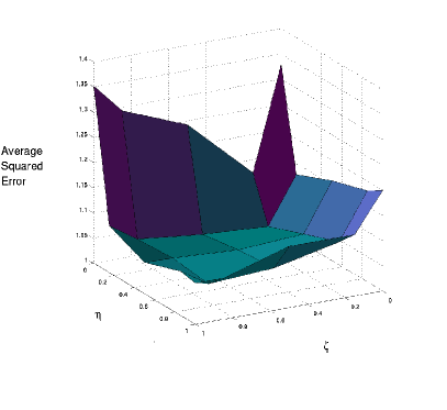
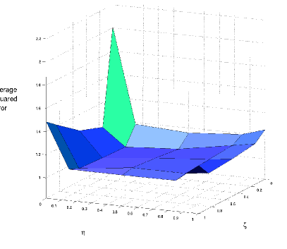
Figure 1: Left: A plot of Mean Squared Error as we vary $\eta$ and $\zeta$. We chose $d$ and $\lambda$ using cross-validation. Right: A plot of Mean Squared Error as we vary $\eta$ and $\zeta$ (for a fixed choice of $\lambda$ and $d$). In both cases we see the performance worsen at the extreme values when either $\eta$ or $\zeta$ become 0.

7 Conclusion

We presented a method for solving a generalized matrix completion problem where we have attributes describing the matrix dimensions. Various approaches, such as standard low rank matrix completion, are special cases of our method, and preliminary experiments confirm the benefits of our method. An interesting direction of future research is to explore further the multi-task learning algorithm we obtained with low-rank constraint. On the theoretical side, a better understanding of the effects of norm and rank regularizations and their interaction would be helpful.

Appendix A Rank of a function in a tensor product RKHS (Section 2.2)

An element of $\mathcal{H}_{\otimes}$ can always be decomposed as a possibly infinite sum of atomic terms of the form $u(x)v(y)$ where $u\in\mathcal{K}$ and $v\in\mathcal{G}$. We define the rank $\text{rank}(f)\in\mathbb{N}\cup\{\infty\}$ of an element $f$ of $\mathcal{H}_{\otimes}$ as the minimal number of atomic terms in any decomposition of $f$, i.e, $\text{rank}(f)$ is the smallest integer $p$ such that $f$ can be expanded as:

$$f\left(\mathbf{x},\mathbf{y}\right)=\sum_{1=1}^{p}u_{i}\left(\mathbf{x}\right)v_{i}\left(\mathbf{y}\right)\;,$$

for some functions $u_{1},\ldots,u_{p}\in\mathcal{K}$ and $v_{1},\ldots,v_{p}\in\mathcal{G}$, if such an integer $p$ does exist (otherwise, the rank is infinite).

When the two RKHS are spaces of linear functions on an Euclidean space, then the tensor product can be identified to the space of bilinear forms on the product of the two Euclidean spaces, and the notion of rank coincides with the usual notion of rank for matrices. We note that an alternative characterization of $\text{rank}(f)$ is the supremum of the ranks of the matrices $M_{i,j}=f\left(\mathbf{x}_{i},\mathbf{y}_{j}\right)$ over the choices of finite sets $\mathbf{x}_{1},\ldots,\mathbf{x}_{m}\in\mathcal{X}$ and $\mathbf{y}_{1},\ldots,\mathbf{y}_{p}\in\mathcal{Y}$ (see technical annex for a proof).

Proposition 4

$\text{rank}(f)$ is equal to the supremum of the ranks of the matrices $M_{i,j}=f\left(\mathbf{x}_{i},\mathbf{y}_{j}\right)$ over the choices of finite sets $\mathbf{x}_{1},\ldots,\mathbf{x}_{m}\in\mathcal{X}$ and $\mathbf{y}_{1},\ldots,\mathbf{y}_{p}\in\mathcal{Y}$.

Proof  If $f$ can be expanded as $\sum_{i=1}^{p}u_{i}\otimes v_{i}$, then for any choice of finite sets $\mathbf{x}_{1},\ldots,\mathbf{x}_{m}\in\mathcal{X}$ and $\mathbf{y}_{1},\ldots,\mathbf{y}_{p}\in\mathcal{Y}$, the matrix $M_{i,j}=f\left(\mathbf{x}_{i},\mathbf{y}_{j}\right)$ can be expanded as $M=\sum_{i=1}^{p}t_{i}w_{i}^{\top}$, where $t_{i,j}=u_{i}(x_{j})$ and $w_{i,j}=v_{i}(y_{j})$, and has therefore a rank not larger than $p$. Taking the smallest possible $p$, this shows that the rank of $M$ can not be larger than the rank of $f$. Conversely, if $f=\sum_{i=1}^{p}u_{i}\otimes v_{i}$ with $\text{rank}(f)=p$, we need to show that there exist two sets of points such that the corresponding matrix $M$ has rank at least $p$. We first observe that both sets $\left(u_{i}\right)_{i=1,\ldots,p}$ and $\left(v_{i}\right)_{i=1,\ldots,p}$ form linearly independent families in $\mathcal{K}$ and $\mathcal{G}$, respectively. Indeed, if for example $u_{p}=\sum_{i=1}^{p-1}r_{i}u_{i}$, then $f(x,y)=\sum_{i=1}^{p-1}u_{i}(x)\left[v_{i}+r_{i}v_{p}\right](y)$ which contradicts the hypothesis that $\text{rank}(f)=p$. It is therefore possible to find to sets of points $\mathbf{x}_{1},\ldots,\mathbf{x}_{p}\in\mathcal{X}$ and $\mathbf{y}_{1},\ldots,\mathbf{y}_{p}\in\mathcal{Y}$, such that the both sets of vectors $\left(t_{i}\right)_{i=1,\ldots,p}$ and $\left(w_{i}\right)_{i=1,\ldots,p}$ form linearly independent families in $\mathbb{R}^{p}$ (where $t_{i,j}=u_{i}(x_{j})$ and $w_{i,j}=v_{i}(y_{j})$). The matrix $M$ corresponding to these sets of points has rank $p$.  

Appendix B Representer theorem with rank constraint (Proof of Proposition 1)

Here we show that the solution of:

$$\min_{f\in\mathcal{H}_{\otimes},\text{ rank}(f)\leqslant p}\left\{\frac{1}{n}\sum_{u=1}^{n}\ell\left(f\left(\mathbf{x}_{i(u)},\mathbf{y}_{j(u)}\right),z_{u}\right)+\lambda\Arrowvert\,f\,\Arrowvert_{\otimes}^{2}\right\}\;,$$ (9)

can be reduced to a finite-dimensional optimization problem:

Proposition 5

The optimal solution of (9) can be written as $f=\sum_{i=1}^{p}u_{i}\otimes v_{i}$, where

$$u_{i}\left(\mathbf{x}\right)=\sum_{l=1}^{n_{\mathcal{X}}}\alpha_{li}k\left({\mathbf{x}}_{l},\mathbf{x}\right)\quad\text{ and }\quad v_{i}\left(\mathbf{y}\right)=\sum_{l=1}^{n_{\mathcal{Y}}}\beta_{li}g\left({\mathbf{y}}_{l},\mathbf{y}\right),\quad i=1,\ldots,p,$$ (10)

where $\alpha\in\mathbb{R}^{n_{\mathcal{X}}\times p}$ and $\beta\in\mathbb{R}^{n_{\mathcal{Y}}\times p}$

Proof  Let $\mathcal{H}_{\otimes}^{S}$ denote the subspace of $\mathcal{H}_{\otimes}$ spanned by the functions $k_{\otimes}\left(\left(x_{i},y_{j}\right),.\right)$ for $i=1,\ldots,n_{\mathcal{X}}$ and $j=1,\ldots,n_{\mathcal{Y}}$, and $\mathcal{H}_{\otimes}^{\perp}$ denote its orthogonal supplement ($\mathcal{H}_{\otimes}=\mathcal{H}_{\otimes}^{S}\oplus\mathcal{H}_{\otimes}^{\perp}$). Similarly, let $\mathcal{K}^{S}$ and $\mathcal{G}^{S}$ denote respectively the subspace of $\mathcal{K}$ and $\mathcal{G}$ spanned by the functions $k\left(\mathbf{x}_{i},.\right)$ for $i=1,\ldots,n_{\mathcal{X}}$, (resp. $g\left(\mathbf{y}_{i},.\right)$ for $i=1,\ldots,n_{\mathcal{Y}}$) and $\mathcal{K}^{\perp}$ and $\mathcal{G}^{\perp}$ the corresponding orthogonal supplements in $\mathcal{K}$ and $\mathcal{G}$. Any function $f\in\mathcal{H}_{\otimes}$ of rank less than $p$ can be expanded as $f=\sum_{i=1}^{p}u_{i}\otimes v_{i}$, with $u_{i}\in\mathcal{K}$ and $v_{i}\in\mathcal{G}$. Now, denote by $u_{i}=u_{i}^{S}+u_{i}^{\perp}$ the unique decomposition of $u_{i}$ over $\mathcal{K}=\mathcal{K}^{S}\oplus\mathcal{K}^{\perp}$, and define similarly $v_{i}=v_{i}^{S}+v_{i}^{\perp}$ with $v_{i}^{S}\in\mathcal{G}^{S}$ and $v_{i}^{\perp}\in\mathcal{G}^{\perp}$. We therefore obtain:

$$f=\sum_{i=1}^{p}u_{i}^{S}\otimes v_{i}^{S}+\sum_{i=1}^{p}u_{i}^{S}\otimes v_{i}^{\perp}+\sum_{i=1}^{p}u_{i}^{\perp}\otimes v_{i}^{S}+\sum_{i=1}^{p}u_{i}^{\perp}\otimes v_{i}^{\perp}.$$ (11)

We now claim that the last three terms in (11) are in $\mathcal{H}_{\otimes}^{\perp}$. Indeed, taking for example a term $u_{i}^{S}\otimes v_{i}^{\perp}$, we have $u_{i}^{S}\otimes v_{i}^{\perp}\left(\mathbf{x}_{j},\mathbf{y}_{l}\right)=u_{i}^{S}\left(\mathbf{x}_{j}\right)v_{i}^{\perp}\left(\mathbf{y}_{l}\right)=0$ because $v_{i}^{\perp}\left(\mathbf{y}_{i}\right)=0$, and therefore $u_{i}^{S}\otimes v_{i}^{\perp}\in\mathcal{H}_{\otimes}^{\perp}$. A similar computation shows that $u_{i}^{\perp}\otimes v_{i}^{S}$ and $u_{i}^{\perp}\otimes v_{i}^{\perp}$ are both in $\mathcal{H}_{\otimes}^{\perp}$. On the other hand, because $u_{i}^{S}\in\mathcal{K}^{S}$ and $v_{i}^{S}\in\mathcal{G}^{S}$, one easily gets that $u_{i}^{S}\otimes v_{i}^{S}\in\mathcal{H}_{\otimes}^{S}$. Therefore $\sum_{i=1}^{p}u_{i}^{S}v_{i}^{S}$ is the orthogonal projection of $s$ onto $\mathcal{H}_{\otimes}^{S}$ and is of rank at most $p$. We can conclude like for the classical representer theorem that is $f$ is not restricted to $\sum_{i=1}^{p}u_{i}^{S}v_{i}^{S}$, then $\sum_{i=1}^{p}u_{i}^{S}v_{i}^{S}$ provides a rank $p$ function of $\mathcal{H}_{\otimes}$ with a strictly smaller functional value, leading to a contradiction.  

Appendix C Representer theorems and trace norm (proof of Proposition 2)

Here we show a representer theorem for the solution of:

$$\min_{f\in\mathcal{H}_{\otimes}}\left\{\frac{1}{n}\sum_{u=1}^{n}\ell\left(f\left(\mathbf{x}_{i(u)},\mathbf{y}_{j(u)}\right),z_{u}\right)+\mu\|(f(\mathbf{x}_{i},\mathbf{y}_{j}))\|_{\ast}+\lambda\Arrowvert\,f\,\Arrowvert_{\otimes}^{2}\right\}\;.$$ (12)

Proposition 6

The optimal solution of (12) can be written in the form $f(x,y)=\sum_{i=1}^{n_{\mathcal{X}}}\sum_{j=1}^{n_{\mathcal{Y}}}\gamma_{ij}k(x,x_{i})k(y,y_{j})$, where $\gamma\in\mathbb{R}^{n_{\mathcal{X}}\times n_{\mathcal{Y}}}$.

Proof  Our objective function is the sum of a function of values of $f$ for all pairs $(x_{i},y_{j})$ plus a squared RKHS norm. The usual representer in the RKHS associated with $k_{\otimes}$ then applies, and we get a solution of the form $f(x,y)=\sum_{i=1}^{n_{\mathcal{X}}}\sum_{j=1}^{n_{\mathcal{Y}}}\gamma_{ij}k_{\otimes}((x,y),(x_{i},y_{j}))=\sum_{i=1}^{n_{\mathcal{X}}}\sum_{j=1}^{n_{\mathcal{Y}}}\gamma_{ij}k(x,x_{i})k(y,y_{j})$ where $\gamma\in\mathbb{R}^{n_{\mathcal{X}}\times n_{\mathcal{Y}}}$.  

Appendix D Learning the kernels (proof of Proposition 3)

In this section we prove that if the loss $\ell$ is convex, then, as a function of the kernel matrices, the optimal values of the optimization problems proposed in the paper are convex functions,

Proposition 7

Given $\beta_{1},\dots,\beta_{p}$, the function

$$H:K\mapsto\min_{\alpha}\left\{\frac{1}{n}\sum_{u=1}^{n}\ell\left(\sum_{k=1}^{p}(K\alpha_{k})_{i(u)}(L\beta_{k})_{j(u)},z_{u}\right)+\lambda\sum_{i=1}^{p}\sum_{j=1}^{p}\alpha_{i}^{\top}K\alpha_{j}\beta_{i}^{\top}G\beta_{j}\right\}$$

is convex in $K$.

Proof  Given $\beta$, the objective function is convex and thus (under appropriate classical conditions), the minimum value is equal to the maximum value of the dual problem, obtained by adding variables $q_{u}$ and adding constraints $q_{u}=\sum_{k=1}^{p}(K\alpha_{k})_{i(u)}(L\beta_{k})_{j(u)}$, together with the appropriate Lagrange multipliers. The results follow from derivations obtained in [3, 11].  

Proposition 8

The function

$$H:(K,G)\mapsto\min_{\gamma\in\mathbb{R}^{n_{\mathcal{X}}\times n_{\mathcal{Y}}}}\left\{\frac{1}{n}\sum_{u=1}^{n}\ell\left((K\gamma G)_{i(u),j(u)},z_{u}\right)+\mu\|K\gamma G\|_{\ast}+\lambda\mathop{\rm tr}\gamma^{\top}K\gamma G\right\}$$ (13)

only depends on the Kronecker product $K\otimes G$ and is a convex function of $K\otimes G$.

Proof  The objective function (13) was originally obtained from (12), which is the sum of a term that is a convex function of the values of a function $f\in\mathcal{H}_{\otimes}$, for all pairs $(\mathbf{x}_{i},\mathbf{y}_{j})$, and the norm $\|f\|^{2}_{\otimes}$. The results of [11] applies to this case and thus the minimum value is a convex function in the kernel matrix for all pairs $(\mathbf{x}_{i},\mathbf{y}_{j})$ and the kernel $k_{\otimes}$, which is exactly $K\otimes G$.

References

- [1] A. Argyriou, T. Evgeniou, and M. Pontil. Multi-task feature learning. In Adv. NIPS 19, 2007.
- [2] N. Aronszajn. Theory of reproducing kernels. Trans. Am. Math. Soc., 68:337 – 404, 1950.
- [3] F. R. Bach, G. R. G. Lanckriet, and M. I. Jordan. Multiple kernel learning, conic duality, and the SMO algorithm. In Proc. ICML, 2004.
- [4] C. Berg, J. P. R. Christensen, and P. Ressel. Harmonic analysis on semigroups. Springer-Verlag, New-York, 1984.
- [5] J. F. Bonnans, J. C. Gilbert, C. Lemaréchal, and C. A. Sagastiz bal. Numerical Optimization Theoretical and Practical Aspects. Springer, 2003.
- [6] S. Boyd and L. Vandenberghe. Convex Optimization. Cambridge Univ. Press, 2003.
- [7] T. Evgeniou, C. Micchelli, and M. Pontil. Learning multiple tasks with kernel methods. J. Mach. Learn. Res., 6:615–637, 2005.
- [8] M. Fazel, H. Hindi, and S. Boyd. A rank minimization heuristic with application to minimum order system approximation. In Proc. American Control Conference, volume 6, 2001.
- [9] G. S. Kimeldorf and G. Wahba. Some results on Tchebycheffian spline functions. J. Math. Anal. Appl., 33:82–95, 1971.
- [10] A. S. Lewis and H. S. Sendov. Twice differentiable spectral functions. SIAM J. Mat. Anal. App., 23(2):368–386, 2002.
- [11] C. A. Micchelli and M. Pontil. Learning the kernel function via regularization. J. Mach. Learn. Res., 6:1099–1125, 2005.
- [12] J. D. M. Rennie and N. Srebro. Fast maximum margin matrix factorization for collaborative prediction. In Proc. ICML, 2005.
- [13] J. Shawe-Taylor and N. Cristianini. Kernel Methods for Pattern Analysis. Cambridge University Press, 2004.
- [14] N. Srebro and T. S. Jaakkola. Weighted low-rank approximations. In Proc. ICML, 2003.
- [15] N. Srebro, J. D. M. Rennie, and T. S. Jaakkola. Maximum-margin matrix factorization. In Adv. NIPS 17, 2005.