$Revision$ $Date$

Functional Bregman Divergence and
Bayesian Estimation of Distributions

B. A. Frigyik, Purdue University, bfrigyik@math.purdue.edu
S. Srivastava, Univ. of Washington, santosh@amath.washington.edu
M. R. Gupta, Univ. of Washington, gupta@ee.washington.edu

Abstract

A class of distortions termed functional Bregman divergences is defined, which includes squared error and relative entropy. A functional Bregman divergence acts on functions or distributions, and generalizes the standard Bregman divergence for vectors and a previous pointwise Bregman divergence that was defined for functions. A recently published result showed that the mean minimizes the expected Bregman divergence. The new functional definition enables the extension of this result to the continuous case to show that the mean minimizes the expected functional Bregman divergence over a set of functions or distributions. It is shown how this theorem applies to the Bayesian estimation of distributions. Estimation of the uniform distribution from independent and identically drawn samples is used as a case study.

1. Overview

Bregman divergences are a useful set of distortion functions that include squared error, relative entropy, logistic loss, Mahalanobis distance, and the Itakura-Saito function. Bregman divergences are popular in statistical estimation and information theory. Analysis using the concept of Bregman divergences has played a key role in recent advances in statistical learning [1, 2, 3, 4, 5, 6, 7, 8, 9], clustering [10, 11], inverse problems [12], maximum entropy estimation [13], and the applicability of the data processing theorem [14]. Recently, it was discovered that the mean is the minimizer of the expected Bregman divergence for a set of $d$-dimensional points [15, 10].

In this paper we define a functional Bregman divergence that applies to functions and distributions, and we show that this new definition is equivalent to Bregman divergence applied to vectors. The functional definition generalizes a pointwise Bregman divergence that has been previously defined for measurable functions [7, 16], and thus extends the class of distortion functions that are Bregman divergences; see Section 2.1.2 for an example. Most importantly, the functional definition enables one to solve functional minimization problems using standard methods from the calculus of variations; we extend the recent result on the expectation of vector Bregman divergence [15, 10] to show that the mean minimizes the expected Bregman divergence for a set of functions or distributions. We show how this theorem links to Bayesian estimation of distributions. For distributions from the exponential family distributions, many popular divergences, such as relative entropy, can be expressed as a (different) Bregman divergence on the exponential distribution parameters. The functional Bregman definition enables stronger results and a more general application.

In Section 1 we state a functional definition of the Bregman divergence and give examples for total squared difference, relative entropy, and squared bias. The relationship between the functional definition and previous Bregman definitions is established. In Section 2 we present the main theorem: that the expectation of a set of functions minimizes the expected Bregman divergence. In Section 3 we discuss the role of this theorem in Bayesian estimation, and as a case study compare different estimates for the uniform distribution given independent and identically drawn samples. For ease of reference, Appendix A contains relevant definitions and results from functional analysis and the calculus of variations. In Appendix B we show that the functional Bregman divergence has many of the same properties as the standard vector Bregman divergence. Proofs are in Appendix C.

2. Functional Bregman Divergence

Let $\left(\mathbb{R}^{d},\Omega,\nu\right)$ be a measure space, where $\nu$ is a Borel measure, $d$ is a positive integer, and define a set of functions $\mathcal{A}=\left\{a\in L^{p}(\nu)\mathop{\hbox{\rm subject to}\;}a:\mathbb{R}^{d}\to\mathbb{R},\;a\geq 0\right\}$ where $1\leq p\leq\infty$.

Definition 2.1 (Functional Definition of Bregman Divergence).

Let $\phi:L^{p}(\nu)\rightarrow\mathbb{R}$ be a strictly convex, twice-continuously Fréchet-differentiable functional. The Bregman divergence $d_{\phi}:\mathcal{A}\times\mathcal{A}\rightarrow[0,\infty)$ is defined for all $f,g\in\mathcal{A}$ as

(1) $$d_{\phi}[f,g]=\phi[f]-\phi[g]-\delta\phi[g;f-g],$$

where $\delta\phi[g;\cdot]$ is the Fréchet derivative of $\phi$ at $g$.

Here, we have used the Fréchet derivative, but the definition (and results in this paper) can be easily extended using more general definitions of derivatives; a sample extension is given in Section 2.1.3.

The functional Bregman divergence has many of the same properties as the standard vector Bregman divergence, including non-negativity, convexity, linearity, equivalence classes, linear separation, dual divergences, and a generalized Pythagorean inequality. These properties are established in Appendix B.

2.1. Examples

Different choices of the functional $\phi$ lead to different Bregman divergences. Illustrative examples are given for squared error, squared bias, and relative entropy. Functionals for other Bregman divergences can be derived based on these examples, from the example functions for the discrete case given in Table 1 of [15], and from the fact that $\phi$ is a strictly convex functional if it has the form $\phi(g)=\int\tilde{\phi}(g(t))dt$ where $\tilde{\phi}:\mathbb{R}\rightarrow\mathbb{R}$, $\tilde{\phi}$ is strictly convex and $g$ is in some well-defined vector space of functions [17].

2.1.1. Total Squared Difference

Let $\phi[g]=\int g^{2}d\nu$, where $\phi:L^{2}(\nu)\to\mathbb{R}$, and let $g,f,a\in L^{2}(\nu)$. Then

$$\phi[g+a]-\phi[g] = \int(g+a)^{2}d\nu-\int g^{2}d\nu$$

$$= 2\int gad\nu+\int a^{2}d\nu.$$

Because

$$\frac{\int a^{2}d\nu}{\|a\|_{L^{2}(\nu)}}=\frac{\|a\|_{L^{2}(\nu)}^{2}}{\|a\|_{L^{2}(\nu)}}=\|a\|_{L^{2}(\nu)}\to 0$$

as $a\to 0$ in $L^{2}(\nu)$,

$$\delta\phi[g;a]=2\int gad\nu,$$

which is a continuous linear functional in $a$. Then, by definition of the second Fréchet derivative,

$$\delta^{2}\phi[g;b,a] = \delta\phi[g+b;a]-\delta\phi[g;a]$$

$$= 2\int(g+b)ad\nu-2\int gad\nu$$

$$= 2\int bad\nu.$$

Thus $\delta^{2}\phi[g;b,a]$ is a quadratic form, where $\delta^{2}\phi$ is actually independent of $g$ and strongly positive since

$$\delta^{2}\phi[g;a,a]=2\int a^{2}d\nu=2\|a\|_{L^{2}(\nu)}^{2}$$

for all $a\in L^{2}(\nu)$, which implies that $\phi$ is strictly convex and

$$d_{\phi}[f,g] = \int f^{2}d\nu-\int g^{2}d\nu-2\int g(f-g)d\nu$$

$$= \int(f-g)^{2}d\nu$$

$$= \|f-g\|_{L^{2}(\nu)}^{2}.$$

2.1.2. Squared Bias

Under definition (1), squared bias is a Bregman divergence, this we have not previously seen noted in the literature despite the importance of minimizing bias in estimation [18].

Let $\phi[g]=\left(\int gd\nu\right)^{2}$, where $\phi:L^{1}(\nu)\to\mathbb{R}$. In this case

(2) $$\phi[g+a]-\phi[g] = \left(\int gd\nu+\int ad\nu\right)^{2}-\left(\int gd\nu\right)^{2}$$

$$= 2\int gd\nu\int ad\nu+\left(\int ad\nu\right)^{2}.$$

Note that $2\int gd\nu\int ad\nu$ is a continuous linear functional on $L^{1}(\nu)$ and $\left(\int ad\nu\right)^{2}\leq\|a\|_{L^{1}(\nu)}^{2}$, so that

$$0\leq\frac{\left(\int ad\nu\right)^{2}}{\|a\|_{L^{1}(\nu)}}\leq\frac{\|a\|_{L^{1}(\nu)}^{2}}{\|a\|_{L^{1}(\nu)}}=\|a\|_{L^{1}(\nu)}.$$

Thus from (2) and the definition of the Fréchet derivative,

$$\delta\phi[g;a]=2\int gd\nu\int ad\nu.$$

By the definition of the second Fréchet derivative,

$$\delta^{2}\phi[g;b,a] = \delta\phi[g+b;a]-\delta\phi[g;a]$$

$$= 2\int(g+b)d\nu\int ad\nu-2\int gd\nu\int ad\nu$$

$$= 2\int bd\nu\int ad\nu$$

is another quadratic form, and $\delta^{2}\phi$ is independent of $g$.

Because the functions in $\mathcal{A}$ are positive, $\delta^{2}\phi$ is strongly positive on $\mathcal{A}$ (which again implies that $\phi$ is strictly convex):

$$\delta^{2}\phi[g;a,a]=2\left(\int ad\nu\right)^{2}=2\|a\|_{L^{1}(\nu)}^{2}\geq 0$$

for $a\in\mathcal{A}$. The Bregman divergence is thus

$$d_{\phi}[f,g]$$

$$= \left(\int fd\nu\right)^{2}-\left(\int gd\nu\right)^{2}-2\int gd\nu\int(f-g)d\nu$$

$$= \left(\int fd\nu\right)^{2}+\left(\int gd\nu\right)^{2}-2\int gd\nu\int fd\nu$$

$$= \left(\int(f-g)d\nu\right)^{2}$$

$$\leq \|f-g\|_{L^{1}(\nu)}^{2}.$$

2.1.3. Relative Entropy of Simple Functions

Let $(X,\Sigma,\nu)$ be a measure space. We denote by $\mathcal{S}$ the collection of all measurable simple functions on $(X,\Sigma,\nu)$, that is, the set of functions which can be written as a finite linear combination of indicator functions. If $g\in\mathcal{S}$ then it can be expressed as

$$g(x)=\sum_{i=0}^{t}\alpha_{i}I_{T_{i}};\quad\alpha_{0}=0,$$

where $I_{T_{i}}$ is the indicator function of the set $T_{i}$ and $\{T_{i}\}_{i=0}^{t}$ is a collection of mutually disjoint measurable sets with the property that $X=\bigcup_{i=0}^{t}T_{i}$. We adopt the convention, that $T_{0}$ is the set on which $g$ is zero and therefore $\alpha_{i}\neq 0$ if $i\neq 0$. The set $\left(\mathcal{S},\|\cdot\|_{L^{\infty}(\nu)}\right)$ is a normed vector space. In this case

(3) $$\int_{X}g\ln gd\nu=\sum_{i=1}^{t}\int_{T_{i}}\alpha_{i}\ln\alpha_{i}d\nu,$$

since $0\ln 0=0$.

Note that the integral in (3) exists and is finite for $g\in\mathcal{S}$ if $g\in L^{1}(\nu)$ and $g\geq 0$. This implies that $\nu(T_{i})<\infty$ for all $1\leq i\leq t$, while the measure of $T_{0}$ could be infinity. For this reason, consider the normed vector space $(L^{1}(\nu)\cap\mathcal{S},$$\|\cdot\|_{L^{\infty}(\nu)})$, where $(L^{1}(\nu)\cap\mathcal{S})$$\subset\mathcal{S}$$\subset L^{\infty}(\nu)$. Let $\mathcal{W}$ be the set (not necessarily a vector space) of functions satisfying the conditions mentioned above – that is, let

$$\mathcal{W}=\{g\in L^{1}(\nu)\cap\mathcal{S}\mathop{\hbox{\rm subject to}\;}g\geq 0\}.$$

Define the functional $\phi$ on $\mathcal{W}$,

(4) $$\phi[g]=\int_{X}g\ln g\,d\nu,\quad g\in\mathcal{W}.$$

The functional $\phi$ is not Fréchet-differentiable at $g$ because in general it cannot be guaranteed that $g+h$ is non-negative for all functions $h$ in the underlying normed vector space $\left(L^{1}(\nu)\cap\mathcal{S},\|\cdot\|_{L^{\infty}(\nu)}\right)$ with norm smaller than any prescribed $\epsilon>0$. However, a generalized Gâteaux derivative can be defined if we limit the perturbing function $h$ to a vector subspace.

Let $\mathcal{G}$ be the subspace of $\left(L^{1}(\nu)\cap\mathcal{S},\|\cdot\|_{L^{\infty}(\nu)}\right)$ defined by

$$\mathcal{G}=\{f\in L^{1}(\nu)\cap\mathcal{S}\mathop{\hbox{\rm subject to}\;}f\,d\nu\ll g\,d\nu\}.$$

It is straightforward to show that $\mathcal{G}$ is vector space. We define the generalized Gâteaux derivative of $\phi$ at $g\in\mathcal{W}$ to be the linear operator $\delta_{G}\phi[g;\cdot]$ if

(5) $$\lim_{\begin{subarray}{c}\|h\|_{L^{\infty}(\nu)}\to 0\\ h\in\mathcal{G}\end{subarray}}\frac{\left|\phi[g+h]-\phi[g]-\delta_{G}\phi[g;h]\right|}{\|h\|_{L^{\infty}(\nu)}}=0.$$

Note, that $\delta_{G}\phi[g;\cdot]$ is not linear in general, but it is on the vector space $\mathcal{G}$. In general, if $\mathcal{G}$ is the entire underlying vector space then (5) is the Fréchet derivative, and if $\mathcal{G}$ is the span of only one element from the underlying vector space then (5) is the Gâteaux derivative. Here, we have generalized the Gâteaux derivative for the present case that $\mathcal{G}$ is a subspace of the underlying vector space.

It remains to be shown that given the functional (4), the derivative (5) exists and yields relative entropy. Consider the solution

(6) $$\delta_{G}\phi[g;h]=\int_{X}(1+\ln g)hd\nu,$$

which coupled with (4) does yield relative entropy. We complete the proof by showing that (6) satisfies (5). Note that

$$\phi[g+h]-\phi[g]-\delta_{G}\phi[g;h] =\int_{X}(h+g)\ln\frac{h+g}{g}-hd\nu$$

(7) $$=\int_{E}(h+g)\ln\frac{h+g}{g}-hd\nu,$$

where $E$ is the set on which $g$ is not zero.

Because $g\in\mathcal{W}$, there are $m,M>0$ such that $m\leq g\leq M$ on $E$. Let $h\in\mathcal{G}$ be such that $\|h\|_{L^{\infty}(\nu)}\leq m$, then $g+h\geq 0$. Our goal is to find a lower and an upper bound for the expression

$$\frac{\phi[g+h]-\phi[g]-\delta_{G}\phi[g;h]}{\|h\|_{L^{\infty}(\nu)}}$$

such that both bounds go to $0$ as $\|h\|_{L^{\infty}(\nu)}\to 0$. We start with bounding the integrand from above:

$$(h+g)\ln\frac{h+g}{g}-h\leq(h+g)\frac{h}{g}-h=\frac{h^{2}}{g},$$

and therefore

$$\frac{\phi[g+h]-\phi[g]-\delta_{G}\phi[g;h]}{\|h\|_{L^{\infty}(\nu)}} \leq \frac{1}{\|h\|_{L^{\infty}(\nu)}}\int_{E}\frac{h^{2}}{g}d\nu$$

$$\leq \frac{1}{m}\int_{E}\left|h\right|d\nu$$

$$\leq \frac{1}{m}\|h\|_{L^{1}(\nu)}.$$

We can use Jensen’s inequality to find a lower bound for the integral (7). In order to use the inequality we have to rewrite the equation. We begin with the first term of the integrand,

$$\int_{E}(h+g)\ln\frac{h+g}{g}d\nu$$

$$= \int_{E}\frac{h+g}{g}\left(\ln\frac{h+g}{g}\right)gd\nu,$$

$$= \|g\|_{L^{1}(\nu)}\int_{E}\frac{h+g}{g}\ln\frac{h+g}{g}\frac{g}{\|g\|_{L^{1}(\nu)}}d\nu$$

$$= \|g\|_{L^{1}(\nu)}\int_{E}\lambda\left(\frac{h+g}{g}\right)d\tilde{\nu},$$

where the measure $d\tilde{\nu}=\frac{g}{\|g\|_{L^{1}(\nu)}}d\nu$ is a probability measure and $\lambda(x)=x\ln x$ is a convex function on $(0,\infty)$. Let $M_{0}=\|g\|_{L^{1}(\nu)}$. By Jensen’s inequality

$$M_{0}\int_{E}\lambda\left(\frac{h+g}{g}\right)d\tilde{\nu}$$

$$\geq M_{0}\lambda\left(\int_{E}\frac{h+g}{g}d\tilde{\nu}\right)$$

$$= M_{0}\lambda\left(\int_{E}\frac{h}{M_{0}}d\nu+\int_{E}d\tilde{\nu}\right)$$

$$= M_{0}\lambda\left(\frac{1}{M_{0}}\int_{E}h\,d\nu+1\right)$$

$$= \left(\int_{E}h\,d\nu+M_{0}\right)\ln\left(\frac{1}{M_{0}}\int_{E}h\,d\nu+1\right).$$

Thus we can bound the integral in (7) from below:

$$\int_{E}(h+g)\ln\frac{h+g}{g}-hd\nu$$

$$\geq \left(\int_{E}h\,d\nu+M_{0}\right)\ln\left(\frac{1}{M_{0}}\int_{E}h\,d\nu+1\right)-\int_{E}h\,d\nu$$

$$= \int_{E}h\,d\nu\ln\left(\frac{1}{M_{0}}\int_{E}h\,d\nu+1\right)$$

$$+M_{0}\ln\left(\frac{1}{M_{0}}\int_{E}h\,d\nu+1\right)-\int_{E}h\,d\nu.$$

If $\int_{E}h\,d\nu=0$, then the integral in (7) is non-negative. The more interesting case is when $\int_{E}h\,d\nu\neq 0$. Then,

$$\frac{\phi[g+h]-\phi[g]-\delta_{G}\phi[g;h]}{\|h\|_{L^{\infty}(\nu)}}$$

$$\geq \frac{\int_{E}h\,d\nu}{\|h\|_{L^{\infty}(\nu)}}\ln\left(\frac{1}{M_{0}}\int_{E}h\,d\nu+1\right)$$

$$+\frac{M_{0}}{\|h\|_{L^{\infty}(\nu)}}\ln\left(\frac{1}{M_{0}}\int_{E}h\,d\nu+1\right)-\frac{\int_{E}h\,d\nu}{\|h\|_{L^{\infty}(\nu)}}$$

$$\geq \frac{\int_{E}h\,d\nu}{\|h\|_{L^{\infty}(\nu)}}\ln\left(\frac{1}{M_{0}}\int_{E}h\,d\nu+1\right)$$

$$+\left[\frac{M_{0}\ln\left(\frac{1}{M_{0}}\int_{E}h\,d\nu+1\right)}{\int_{E}h\,d\nu}-1\right]\frac{\int_{E}h\,d\nu}{\|h\|_{L^{\infty}(\nu)}}.$$

As $\int_{E}h\,d\nu\to 0$,

$$\ln\left(\frac{1}{M_{0}}\int_{E}h\,d\nu+1\right)\to 0,$$

and

$$\frac{M_{0}\ln\left(\frac{1}{M_{0}}\int_{E}h\,d\nu+1\right)}{\int_{E}h\,d\nu}-1\to 0.$$

We finish the proof by showing that there is a constant $K$ which is independent of $h$ such that

(8) $$\left|\int_{E}h\,d\nu\right|\leq\|h\|_{L^{1}(\nu)}\leq K\|h\|_{L^{\infty}(\nu)}.$$

If (8) is shown, then $\int_{E}h\,d\nu\to 0$ and $\|h\|_{L^{1}(\nu)}\to 0$ as $\|h\|_{L^{\infty}(\nu)}\to 0$, and coupling those relationships with the fact that

$$\frac{\left|\int_{E}h\,d\nu\right|}{\|h\|_{L^{\infty}(\nu)}}\leq K$$

establishes (5). Because $h\in\mathcal{G}$, $h$ can be expressed as

$$h=\sum_{i=0}^{v}\beta_{i}I_{V_{i}};\quad\beta_{0}=0,$$

where $\{V_{i}\}_{i=0}^{v}$ is a collection of mutually disjoint measurable sets with the property that $X=\bigcup_{i=0}^{v}V_{i}$. Also, because $h\,d\nu\ll g\,d\nu$, there is a set $N(h)$ such that $\nu(N(h))=0$ and

$$\bigcup_{i=1}^{v}V_{i}\subset\left(\bigcup_{i=1}^{t}T_{i}\cup N(h)\right).$$

This implies that there is a $K$ independent of $h$ such that

$$\sum_{i=1}^{v}\nu(V_{i})\leq\sum_{i=1}^{t}\nu(T_{i})=K.$$

Finally,

$$\int\left|h\right|d\nu = \sum_{i=1}^{v}\left|\beta_{i}\right|\nu(V_{i})$$

$$\leq \|h\|_{L^{\infty}(\nu)}\sum_{i=1}^{v}\nu(V_{i})$$

$$\leq \|h\|_{L^{\infty}(\nu)}K.$$

2.2. Relationship to Other Bregman Divergence Definitions

Two propositions establish the relationship of the functional Bregman divergence to other Bregman divergence definitions.

Proposition 2.2 (Functional Bregman Divergence Generalizes Vector Bregman Divergence).

The functional definition (1) is a generalization of the standard vector Bregman divergence

(9) $$d_{\tilde{\phi}}(x,y)=\tilde{\phi}(x)-\tilde{\phi}(y)-\nabla\tilde{\phi}(y)^{T}(x-y),$$

where $x,y\in\mathbb{R}^{n}$, and $\tilde{\phi}:\mathbb{R}^{n}\to\mathbb{R}$ is strictly convex and twice differentiable.

Jones and Byrne describe a general class of divergences between functions using a pointwise formulation [7]. Csiszár specialized the pointwise formulation to a class of divergences he termed Bregman distances $B_{s,\nu}$ [16], where given a $\sigma$-finite measure space $(X,\Omega,\nu)$, and non-negative measurable functions $f(x)$ and $g(x)$, $B_{s,\nu}(f,g)$ equals

(10) $$\int s(f(x))-s(g(x))-s^{\prime}(g(x))(f(x)-g(x))d\nu(x).$$

The function $s:(0,\infty)\rightarrow\mathbb{R}$ is constrained to be differentiable and strictly convex, and the limit $\lim_{x\rightarrow 0}s(x)$ and $\lim_{x\rightarrow 0}s^{\prime}(x)$ must exist, but not necessarily finite. The function $s$ plays a role similar to the function $\phi$ in the functional Bregman divergence; however, $s$ acts on the range of the functions $f,g$, whereas $\phi$ acts on the pair of functions $f,g$.

Proposition 2.3 (Functional Definition Generalizes Pointwise Definition).

Given a pointwise Bregman divergence as per (10), an equivalent functional Bregman divergence can be defined as per (1) if the measure $\nu$ is finite. However, given a functional Bregman divergence $d_{\phi}[f,g]$, there is not necessarily an equivalent pointwise Bregman divergence.

3. Minimum Expected Bregman Divergence

Consider two sets of functions (or distributions), $\mathcal{M}$ and $\mathcal{A}$. Let $F\in\mathcal{M}$ be a random function with realization $f$. Suppose there exists a probability distribution $P_{F}$ over the set $\mathcal{M}$, such that $P_{F}(f)$ is the probability of $f\in\mathcal{M}$. For example, consider the set of Gaussian distributions, and given samples drawn independently and identically from a randomly selected Gaussian distribution $N$, the data imply a posterior probability $P_{N}(\mathcal{N})$ for each possible generating realization of a Gaussian distribution $\mathcal{N}$. The goal is to find the function $g^{*}\in\mathcal{A}$ that minimizes the expected Bregman divergence between the random function $F$ and any function $g\in\mathcal{A}$. The following theorem shows that if the set of possible minimizers $\mathcal{A}$ includes $E_{P_{F}}[F]$, then $g^{*}=E_{P_{F}}[F]$ minimizes the expectation of any Bregman divergence.

The theorem applies only to a set of functions $\mathcal{M}$ that lie on a finite-dimensional manifold $M$ for which a differential element $dM$ can be defined. For example, the set $\mathcal{M}$ could be parameterized by a finite number of parameters, or could be a set of functions that can be decomposed into a finite set of $d$ basis functions $\{\psi_{1},\psi_{2},\ldots,\psi_{d}\}$ such that each $f$ can be expressed as

$$f=\sum_{j=1}^{d}c_{j}\psi_{j},$$

where $c_{j}\in\mathbb{R}$ for all $j$. The theorem requires slightly stronger conditions on $\phi$ than the definition of the Bregman divergence (1) requires.

Theorem 3.1 (Minimizer of the Expected Bregman Divergence).

Let $\delta^{2}\phi[f;a,a]$ be a strongly positive quadratic form, and let $\phi\in\mathcal{C}^{3}(L^{1}(\nu);\mathbb{R})$ be a three-times continuously Fréchet-differentiable functional on $L^{1}(\nu)$. Let $\mathcal{M}$ be a set of functions that lie on a finite-dimensional manifold $M$, and have associated differential element $dM$. Suppose there is a probability distribution $P_{F}$ defined over the set $\mathcal{M}$. Suppose the function $g^{*}$ minimizes the expected Bregman divergence between the random function $F$ and any function $g\in\mathcal{A}$ such that

$$g^{*}=\arg\inf_{g\in\mathcal{A}}E_{P_{F}}[d_{\phi}(F,g)].$$

Then, if $g^{*}$ exists, it is given by

(11) $$g^{*}=\int_{M}fP(f)dM=E_{P_{F}}[F].$$

4. Bayesian Estimation

Theorem II.1 can be applied to a set of distributions to find the Bayesian estimate of a distribution given a posterior or likelihood. For parametric distributions parameterized by $\theta\in\mathbb{R}^{n}$, a probability measure $\Lambda(\theta)$, and some risk function $R(\theta,\psi)$, $\psi\in\mathbb{R}^{n}$, the Bayes estimator is defined [19] as

(12) $$\hat{\theta}=\arg\inf_{\psi\in\mathbb{R}^{n}}\int R(\theta,\psi)d\Lambda(\theta).$$

That is, the Bayes estimator minimizes some expected risk in terms of the parameters. It follows from recent results [15] that $\hat{\theta}=E[\Theta]$ if the risk $R$ is a Bregman divergence, where $\Theta$ is the random variable whose realization is $\theta$.

The principle of Bayesian estimation can be applied to the distributions themselves rather than to the parameters:

(13) $$\hat{g}=\arg\inf_{g\in\mathcal{A}}\int_{M}R(f,g)P_{F}(f)dM,$$

where $P_{F}(f)$ is a probability measure on the distributions $f\in\mathcal{M}$, $dM$ is a differential element for the finite-dimensional manifold $M$, and $\mathcal{A}$ is either the space of all distributions or a subset of the space of all distributions, such as the set $\mathcal{M}$. When the set $\mathcal{A}$ includes the distribution $E_{P_{F}}[F]$ and the risk function $R$ in (13) is a Bregman divergence, then Theorem II.1 establishes that $\hat{g}=E_{P_{F}}[F]$.

For example, in recent work, two of the authors derived the mean class posterior distribution for each class for a Bayesian quadratic discriminant analysis classifier [6], and showed that the classification results were superior to parameter-based Bayesian quadratic discriminant analysis.

Of particular interest for estimation problems are the Bregman divergence examples given in Section 2.1: total squared difference (mean squared error) is a popular risk function in regression [18]; minimizing relative entropy leads to useful theorems for large deviations and other statistical subfields [20]; and analyzing bias is a common approach to characterizing and understanding statistical learning algorithms [18].

4.1. Case Study: Estimating a Scaled Uniform Distribution

As an illustration, we present and compare different estimates of a scaled uniform distribution given independent and identically drawn samples. Let the set of uniform distributions over $[0,\theta]$ for $\theta\in\mathbb{R}^{+}$ be denoted by $\mathcal{U}$. Given independent and identically distributed samples $X_{1},X_{2},\ldots,X_{n}$ drawn from an unknown uniform distribution $f\in\mathcal{U}$, the generating distribution is to be estimated. The risk function $R$ is taken to be squared error or total squared error depending on context.

4.1.1. Bayesian Parameter Estimate

Depending on the choice of the probability measure $\Lambda(\theta)$, the integral (12) may not be finite; for example, using the likelihood of $\theta$ with Lebesgue measure the integral is not finite. A standard solution is to use a gamma prior on $\theta$ and Lebesgue measure. Let $\Theta$ be a random parameter with realization $\theta$, let the gamma distribution have parameters $t_{1}$ and $t_{2}$, and denote the maximum of the data as $X_{\max}=\max\{X_{1},X_{2},\ldots,X_{n}\}$. Then a Bayesian estimate is formulated [19, p. 240, 285]:

(14) $$E[\Theta|\{X_{1},X_{2},\ldots,X_{n}\},t_{1},t_{2}]$$

$$= \frac{\int_{X_{\max}}^{\infty}\theta\frac{1}{\theta^{n+t_{1}+1}}e^{\frac{-1}{\theta t_{2}}}d\theta}{\int_{X_{\max}}^{\infty}\frac{1}{\theta^{n+t_{1}+1}}e^{\frac{-1}{\theta t_{2}}}d\theta}.$$

The integrals can be expressed in terms of the chi-squared random variable $I_{v}^{2}$ with $v$ degrees of freedom:

(15) $$E[\Theta|\{X_{1},X_{2},\ldots,X_{n}\},t_{1},t_{2}]=$$

$$\frac{1}{t_{2}(n+t_{1}-a)}\frac{P(\chi^{2}_{2(n+t_{1}-1)}<\frac{2}{t_{2}X_{\max}})}{P(\chi^{2}_{2(n+t_{1})}<\frac{2}{t_{2}X_{\max}})}.$$

Note that (12) presupposes that the best solution is also a uniform distribution.

4.1.2. Bayesian Uniform Distribution Estimate

If one restricts the minimizer of (13) to be a uniform distribution, then (13) is solved with $\mathcal{A}=\mathcal{U}$. Because the set of uniform distributions does not generally include its mean, Theorem II.1 does not apply, and thus different Bregman divergences may give different minimizers for (13). Let $P_{F}$ be the likelihood of the data (no prior is assumed over the set $\mathcal{U}$), and use the Fisher information metric ([21, 22, 23]) for $dM$. Then the solution to (13) is the uniform distribution on $[0,2^{1/n}X_{\max}]$. Using Lebesgue measure instead gives a similar result: $[0,2^{1/(n+1/2)}X_{\max}]$. We were unable to find these estimates in the literature, and so their derivations are presented in Appendix C.

4.1.3. Unrestricted Bayesian Distribution Estimate

When the only restriction placed on the minimizer $g$ in (13) is that $g$ be a distribution, then one can apply Theorem II.1 and solve directly for the expected distribution $E_{P_{F}}[F]$. Let $P_{F}$ be the likelihood of the data (no prior is assumed over the set $\mathcal{U}$), and use the Fisher information metric for $dM$. Solving (11), noting that the uniform probability of $x$ is $f(x)=1/a$ if $x\leq a$ and zero otherwise, and the likelihood of the $n$ drawn points is $(1/X_{\max})^{n}$ if $a\geq X_{\max}$ and zero otherwise,

(16) $$g^{*}(x) = \frac{\int_{\max(x,X_{\max})}^{\infty}\left(\frac{1}{a}\right)\left(\frac{1}{a^{n}}\right)\left(\frac{da}{a}\right)}{\int_{X_{\max}}^{\infty}\frac{1}{a^{n}}\frac{da}{a}}$$

$$= \frac{n\left(X_{\max}\right)^{n}}{(n+1)[\max(x,X_{\max})]^{n+1}}.$$

4.1.4. Projecting the Unrestricted Estimate onto the Set of Uniform Distributions

Consider what happens when the unrestricted solution $g^{*}(x)$ given in (16) is projected onto the set of uniform distributions with respect to squared error. That is, we solve for the uniform distribution $h(x)$ over $[0,a]$ such that:

(17) $$\hat{a}=\arg\min_{a\in[0,\infty)}\int_{0}^{\infty}(h(x)-g^{*}(x))^{2}dx.$$

The problem is straightforward to solve using standard calculus and yields the solution $\hat{a}=2^{1/n}X_{\max}$. This is also the solution to the problem (13) when the minimizer is restricted to be a uniform distribution and the Fisher information metric over the uniform distributions is used (as discussed in Section 4.1.3). Thus, the projection of the unrestricted solution to (13) onto the set of uniform distributions is the same as the solution to (13) when the minimizer is restricted to be uniform. We conjecture that under some conditions this property will hold more generally: that the projection of the unrestricted minimizer of (13) onto the set $\mathcal{M}$ will be equivalent to solving (13) where the solution is restricted to the set $\mathcal{M}$.

4.2. Simulation

A simulation was done to compare the different Bayesian estimators and the maximum likelihood estimator. The simulation was run $1,000$ times; each time $n$ data points were drawn independently and identically from the uniform over $[0,1]$, and estimates were formed. Figure 1 is a log-log plot of the average squared errors between the estimated distribution and the true distribution.

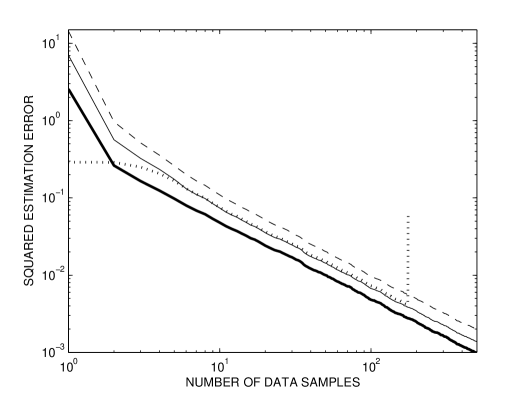
Figure 1. The plot shows the log of the squared error between an estimated distribution and a uniform $[0,1]$ distribution, averaged over one thousand runs of the estimation simulation. The dashed line is the maximum likelihood estimate, the dotted line is the Bayesian parameter estimate, the thick solid line is the Bayesian distribution estimate that solves (13), and the thin solid line is the Bayesian distribution estimate that solves (13) when the minimizer is restricted to be uniform.

For the Bayesian parameter estimator given in (15), estimates were calculated for three different sets of Gamma parameters, $(t_{1}=1,t_{2}=1)$, $(t_{1}=1,t_{2}=3)$, and $(t_{1}=1,t_{2}=100)$. The plotted error is the minimum of the three averaged errors for the different Gamma priors for each $n$. The plotted Bayesian distribution estimates used the Fisher information metric (very similar simulation results were obtained with the Lebesgue measure).

Given more than one random sample from the uniform, the unrestricted Bayesian distribution estimator (thick line) always performed better than the other estimators (as it should by design). Of course, asymptotically as $n\rightarrow\infty$, all of the estimates will converge to the true value. For $n=1$, the Bayesian parameter estimate performs better; we believe this is due to the (in this case correct) bias of the prior used for the Bayesian parameter estimate. The dotted line rises at $n=155$ because the Bayesian parameter estimate was uncomputable for more than $155$ data samples (we used Matlab v. 14 to evaluate (15), and for $155$ data samples or more the numerator and denominator of (15) were determined to be $0$, leading to an indeterminate estimate).

Three interesting conclusions are supported by the simulation results. First, the Bayesian estimates do improve significantly over the maximum likelihood estimate (dashed line). Second, although the truth is uniform, the unrestricted Bayesian distribution estimate chooses a non-uniform solution (thick line), which does significantly better than either of the Bayesian uniform estimates (thin line and dotted line). Third, the Bayesian parameter estimate (dotted line) and the Bayesian uniform distribution estimate (thin line) perform quite similarly. For $n<10$, the Bayesian parameter estimate works better, but for $n>10$, the Bayesian uniform distribution estimate is slightly better. Although these two estimates perform similarly, the Bayesian uniform distribution estimate $[0,2^{1/n}X_{\max}]$ is a more elegant solution than the parameter estimate (15), and is easier to compute and to work with analytically.

5. Further Discussion and Open Questions

We have defined a general Bregman divergence for functions and distributions that can provide a foundation for results in statistics, information theory and signal processing. Theorem II.1 is important for these fields because it ties Bregman divergences to expectation. As shown in Section 4, Theorem II.1 can be directly applied to distributions to show that Bayesian distribution estimation simplifies to expectation when the risk function is a Bregman divergence and the minimizing distribution is unrestricted.

It is common in Bayesian estimation to interpret the prior as representing some actual prior knowledge, but in fact prior knowledge often is not available or is difficult to quantify. Another approach is to use a prior to capture coarse information from the data that may be used to stabilize the estimation [6, 9]. In practice, priors are sometimes chosen in Bayesian estimation to tame the tail of likelihood distributions so that expectations will exist when they might otherwise be infinite [19]. This mathematically convenient use of priors adds estimation bias that may be unwarranted by prior knowledge. An alternative to mathematically convenient priors is to formulate the estimation problem as a minimization of an expected Bregman divergence between the unknown distribution and the estimated distribution, and restrict the set of distributions that can be the minimizer to be a set for which the Bayesian integral exist. Open questions are how such restrictions affect the estimation bias and variance, and how to find or define a “best” restricted set of distributions for this estimation approach.

Finally, there are some results for the standard vector Bregman divergence that have not been extended here. It has been shown that a standard vector Bregman divergence must be the risk function in order for the mean to be the minimizer of an expected risk [15, Theorems 3 and 4]. The proof of that result relies heavily on the discrete nature of the underlying vectors, and it remains an open question as to whether a similar result holds for the functional Bregman divergence. Another result that has been shown for the vector case but remains an open question in the functional case is convergence in probability [15, Theorem 2].

Appendix A: Relevant Definitions and Results from Functional Analysis

This appendix explains the basic definitions and results from functional analysis used in this paper. This material can also be found in standard books on the calculus of variations, such as the text by Gelfand and Fomin [24].

Let $\left(\mathbb{R}^{d},\Omega,\nu\right)$ be a measure space, where $\nu$ is a Borel measure $d$ is a positive integer, and define a set of functions $\mathcal{A}=\left\{a\in L^{p}(\nu)\mathop{\hbox{\rm subject to}\;}a:\mathbb{R}^{d}\to\mathbb{R},\;a\geq 0\right\}$ where $1\leq p\leq\infty$. The subset $\mathcal{A}$ is a convex subset of $L^{p}(\nu)$ because for $a_{1}$, $a_{2}\in\mathcal{A}$ and $0\leq\omega\leq 1$, $\omega a_{1}+(1-\omega)a_{2}\in\mathcal{A}$.

Definition of continuous linear functionals
The functional $\psi:L^{p}(\nu)\to\mathbb{R}$ is linear and continuous if

1. $\psi[\omega a_{1}+a_{2}]=\omega\psi[a_{1}]+\psi[a_{2}]$ for any $a_{1},a_{2}\in L^{p}(\nu)$ and any real number $\omega$; and

2. there is a constant C such that $\left|\psi[a]\right|\leq C\|a\|$ for all $a\in L^{p}(\nu)$.

Functional Derivatives

1. Let $\phi$ be a real functional over the normed space $L^{p}(\nu)$. The bounded linear functional $\delta\phi[f;\cdot]$ is the Fréchet derivative of $\phi$ at $f\in L^{p}(\nu)$ if

   $$\phi[f+a]-\phi[f] =\triangle\phi[f;a]$$

   (18) $$=\delta\phi[f;a]+\epsilon[f,a]\left\|a\right\|_{L^{p}(\nu)}$$

   for all $a\in L^{p}(\nu)$, with $\epsilon[f,a]\rightarrow 0$ as $\left\|a\right\|_{L^{p}(\nu)}\rightarrow 0$.

2. When the second variation $\delta^{2}\phi$ and the third variation $\delta^{3}\phi$ exist, they are described by

   $$\triangle\phi[f;a] = \delta\phi[f;a]+\frac{1}{2}\delta^{2}\phi[f;a,a]$$

   $$\mbox{}+\epsilon[f,a]\left\|a\right\|^{2}_{L^{p}(\nu)}$$

   $$= \delta\phi[f;a]+\frac{1}{2}\delta^{2}\phi[f;a,a]$$

   $$\mbox{}+\frac{1}{6}\delta^{3}\phi[f;a,a,a]$$

   $$\mbox{}+\epsilon[f,a]\left\|a\right\|^{3}_{L^{p}(\nu)},$$

   where $\epsilon[f,a]\rightarrow 0$ as $\left\|a\right\|_{L^{p}(\nu)}\rightarrow 0$. The term $\delta^{2}\phi[f;a,b]$ is bilinear with respect to arguments $a$ and $b$, and $\delta^{3}\phi[f;a,b,c]$ is trilinear with respect to $a,b$, and $c$.

3. Suppose $\{a_{n}\},\{f_{n}\}\subset L^{p}(\nu)$, moreover $a_{n}\rightarrow a$, $f_{n}\rightarrow f$, where $a,f\in L^{p}(\nu)$. If $\phi\in\mathcal{C}^{3}(L^{p}(\nu);\mathbb{R})$ and $\delta\phi[f;a]$, $\delta^{2}\phi[f;a,a]$, and $\delta^{3}[f;a,a,a]$ are defined as above, then $\delta\phi[f_{n};a_{n}]\rightarrow\delta\phi[f;a]$, $\delta^{2}\phi[f_{n};a_{n},a_{n}]\rightarrow\delta^{2}\phi[f;a,a]$, and $\delta^{3}\phi[f_{n};a_{n},a_{n},a_{n}]\rightarrow\delta^{3}\phi[f;a,a,a]$, respectively.

4. The quadratic functional $\delta^{2}\phi[f;a,a]$ defined on normed linear space $L^{p}(\nu)$ is strongly positive if there exists a constant $k>0$ such that $\delta^{2}\phi[f;a,a]\geq k\left\|a\right\|_{L^{p}(\nu)}^{2}$ for all $a\in\mathcal{A}$. In a finite-dimensional space, strong positivity of a quadratic form is equivalent to the quadratic form being positive definite.

5. From (2),

   $$\phi[f+a] = \phi[f]+\delta\phi[f;a]+\frac{1}{2}\delta^{2}\phi[f;a,a]$$

   $$+o(\|a\|^{2}),$$

   $$\phi[f] = \phi[f+a]-\delta\phi[f+a;a]+$$

   $$\frac{1}{2}\delta^{2}\phi[f+a;a,a]+o(\|a\|^{2}),$$

   where $o(\|a\|^{2})$ stands for a function that goes to zero as $\|a\|$ goes to zero, even if it is divided by $\|a\|^{2}$. Adding the above two equations yields

   $$0 = \delta\phi[f;a]-\delta\phi[f+a;a]+\frac{1}{2}\delta^{2}\phi[f;a,a]$$

   $$+\frac{1}{2}\delta^{2}\phi[f+a;a,a]+o(\|a\|{}^{2}),$$

   which is equivalent to

   (20) $$\delta\phi[f+a;a]-\delta\phi[f;a]=\delta^{2}\phi[f;a,a]+o(\|a\|{}^{2}),$$

   because

   $$\left|\delta^{2}\phi[f+a;a,a]-\delta^{2}\phi[f;a,a]\right|\\ \leq\|\delta^{2}\phi[f+a;\cdot,\cdot]-\delta^{2}\phi[f;\cdot,\cdot]\|\|a\|^{2},$$

   and we assumed $\phi\in\mathcal{C}^{2}$, so $\delta^{2}\phi[f+a;a,a]-\delta^{2}\phi[f;a,a]$ is of order $o(\|a\|^{2})$. This shows that the variation of the first variation of $\phi$ is the second variation of $\phi$. A procedure like the above can be used to prove that analogous statements hold for higher variations if they exist.

Functional Optimality Conditions For a functional $J$ to have an extremum (minimum) at $f=\hat{f}$, it is necessary that

$$\delta J[f;a]=0\;\;\mbox{and}\;\;\delta^{2}J[f;a,a]\geq 0,$$

for $f=\hat{f}$ and for all admissible functions $a\in\mathcal{A}$. A sufficient condition for a functional $J[f]$ to have a minimum for $f=\hat{f}$ is that the first variation $\delta J[f;a]$ must vanish for $f=\hat{f}$, and its second variation $\delta^{2}J[f;a,a]$ must be strongly positive for $f=\hat{f}$.

Appendix B: Properties of the Functional Bregman Divergence

The Bregman divergence for random variables has some well-known properties, as reviewed in [10, Appendix A]. Here, we establish that the same properties hold for the functional Bregman divergence (1).
1. Non-negativity
The functional Bregman divergence is non-negative. To show this, define $\tilde{\phi}:\mathbb{R}\to\mathbb{R}$ by $\tilde{\phi}(t)=\phi\left[tf+(1-t)g\right]$, $f,g\in\mathcal{A}$. From the definition of the Fréchet derivative,

(21) $$\frac{d}{dt}{\tilde{\phi}}=\delta\phi[tf+(1-t)g;f-g].$$

The function $\tilde{\phi}$ is convex because $\phi$ is convex by definition. Then from the mean value theorem there is some $0\leq t_{0}\leq 1$ such that

(22) $$\tilde{\phi}(1)-\tilde{\phi}(0)=\frac{d}{dt}{\tilde{\phi}}(t_{0})\geq\frac{d}{dt}{\tilde{\phi}}(0).$$

Because $\tilde{\phi}(1)=\phi[f]$, $\tilde{\phi}(0)=\phi[g]$, and (21), subtracting the right-hand side of (22) implies that

(23) $$\phi[f]-\phi[g]-\delta\phi[g,f-g]\geq 0.$$

If $f=g$, then (23) holds in equality. To finish, we prove the converse. Suppose (23) holds in equality; then

(24) $$\tilde{\phi}(1)-\tilde{\phi}(0)=\frac{d}{dt}{\tilde{\phi}}(0).$$

The equation of the straight line connecting $\tilde{\phi}(0)$ to $\tilde{\phi}(1)$ is $\ell(t)=\tilde{\phi}(0)+(\tilde{\phi}(1)-\tilde{\phi}(0))t$, and the tangent line to the curve $\tilde{\phi}$ at $\tilde{\phi}(0)$ is $y(t)=\tilde{\phi}(0)+t\frac{d}{dt}{\tilde{\phi}}(0)$. Because $\tilde{\phi}(\tau)=\tilde{\phi}(0)+\int_{0}^{\tau}\frac{d}{dt}{\tilde{\phi}}(t)dt$ and $\frac{d}{dt}{\tilde{\phi}}(t)\geq\frac{d}{dt}{\tilde{\phi}}(0)$ as a direct consequence of convexity, it must be that $\tilde{\phi}(t)\geq y(t)$. Convexity also implies that $\ell(t)\geq\tilde{\phi}(t)$. However, the assumption that (23) holds in equality implies (24), which means that $y(t)=\ell(t)$, and thus $\tilde{\phi}(t)=\ell(t)$, which is not strictly convex. Because $\phi$ is by definition strictly convex, it must be true that $\phi[tf+(1-t)g]<t\phi[f]+(1-t)\phi[g]$ unless $f=g$. Thus, under the assumption of equality of (23), it must be true that $f=g$.

2. Convexity
The Bregman divergence $d_{\phi}[f,g]$ is always convex with respect to $f$. Consider

$$\triangle d_{\phi}[f,g;a] = d_{\phi}[f+a,g]-d_{\phi}[f,g]$$

$$= \phi[f+a]-\phi[f]-\delta\phi[g;f-g+a]+$$

$$\delta\phi[g;f-g].$$

Using linearity in the third term,

$$\triangle d_{\phi}[f,g;a]$$

$$= \phi[f+a]-\phi[f]-\delta\phi[g;f-g]-\delta\phi[g;a]$$

$$+\delta\phi[g;f-g],$$

$$= \phi[f+a]-\phi[f]-\delta\phi[g;a],$$

$$\stackrel{{\scriptstyle(a)}}{{=}} \delta\phi[f;a]+\frac{1}{2}\delta^{2}\phi[f;a,a]+\epsilon[f,a]\left\|a\right\|^{2}_{L(\nu)}-\delta\phi[g;a]$$

$$\Rightarrow \delta^{2}d_{\phi}[f,g;a,a]=\frac{1}{2}\delta^{2}\phi[f;a,a]>0,$$

where (a) and the conclusion follows from (2).
3. Linearity
The functional Bregman divergence is linear in the sense that

$$d_{(c_{1}\phi_{1}+c_{2}\phi_{2})}[f,g]$$

$$= (c_{1}\phi_{1}+c_{2}\phi_{2})[f]-(c_{1}\phi_{1}+c_{2}\phi_{2})[g]-$$

$$\delta(c_{1}\phi_{1}+c_{2}\phi_{2})[g;f-g],$$

$$= c_{1}d_{\phi_{1}}[f,g]+c_{2}d_{\phi_{2}}[f,g].$$

4. Equivalence Classes
Partition the set of strictly convex, differentiable functions $\left\{\phi\right\}$ on $\mathcal{A}$ into classes with respect to functional Bregman divergence, so that $\phi_{1}$ and $\phi_{2}$ belong to the same class if $d_{\phi_{1}}[f,g]=d_{\phi_{2}}[f,g]$ for all $f,g\in\mathcal{A}$. For brevity we will denote $d_{\phi_{1}}[f,g]$ simply by $d_{\phi_{1}}$. Let $\phi_{1}\sim\phi_{2}$ denote that $\phi_{1}$ and $\phi_{2}$ belong to the same class, then $\sim$ is an equivalence relation because it satisfies the properties of reflexivity (because $d_{\phi_{1}}=d_{\phi_{1}}$), symmetry (because if $d_{\phi_{1}}=d_{\phi_{2}}$, then $d_{\phi_{2}}=d_{\phi_{1}}$), and transitivity (because if $d_{\phi_{1}}=d_{\phi_{2}}$ and $d_{\phi_{2}}=d_{\phi_{3}}$, then $d_{\phi_{1}}=d_{\phi_{3}}$).

Further, if $\phi_{1}\sim\phi_{2}$, then they differ only by an affine transformation. To see this, note that, by assumption, $\phi_{1}[f]$ $-\phi_{1}[g]$ $-\delta\phi_{1}[g;f-g]$ $=\phi_{2}[f]$$-\phi_{2}[g]$ $-\delta\phi_{2}[g;f-g]$, and fix $g$ so $\phi_{1}[g]$ and $\phi_{2}[g]$ are constants. By the linearity property, $\delta\phi[g;f-g]=\delta\phi[g;f]-\delta\phi[g;g]$, and because $g$ is fixed, this equals $\delta\phi[g;f]+c_{0}$ where $c_{0}$ is a scalar constant. Then $\phi_{2}[f]=\phi_{1}[f]+(\delta\phi_{2}[g;f]-\delta\phi_{1}[g;f])+c_{1}$, where $c_{1}$ is a constant. Thus,

$$\phi_{2}[f]=\phi_{1}[f]+Af+c_{1},$$

where $A=\delta\phi_{2}[g;\cdot]-\delta\phi_{1}[g;\cdot]$, and thus $A:\mathcal{A}\rightarrow\mathbb{R}$ is a linear operator that does not depend on $f$.

5. Linear Separation
Fix two non-equal functions $g_{1},g_{2}\in\mathcal{A}$, and consider the set of all functions in $\mathcal{A}$ that are equidistant in terms of functional Bregman divergence from $g_{1}$ and $g_{2}$:

$$d_{\phi}[f,g_{1}]=d_{\phi}[f,g_{2}]$$

$$\Rightarrow -\phi[g_{1}]-\delta\phi[g_{1};f-g_{1}]=-\phi[g_{2}]-\delta\phi[g_{2};f-g_{2}]$$

$$\Rightarrow -\delta\phi[g_{1};f-g_{1}]=\phi[g_{1}]-\phi[g_{2}]-\delta\phi[g_{2};f-g_{2}].$$

Using linearity the above relationship can be equivalently expressed as

$$-\delta\phi[g_{1};f]+\delta\phi[g_{1};g_{1}] = \phi[g_{1}]-\phi[g_{2}]-\delta\phi[g_{2};f]+$$

$$\delta\phi[g_{2};g_{2}],$$

$$\delta\phi[g_{2};f]-\delta\phi[g_{1};f] = \phi[g_{1}]-\phi[g_{2}]-\delta\phi[g_{1};g_{1}]+$$

$$\delta\phi[g_{2};g_{2}].$$

$$Lf = c,$$

where $L$ is the bounded linear functional defined by $Lf=\delta\phi[g_{2};f]-\delta\phi[g_{1};f]$, and $c$ is the constant corresponding to the right-hand side. In other words, $f$ has to be in the set $\{a\in\mathcal{A}:La=c\}$, where $c$ is a constant. This set is a hyperplane.

6. Dual Divergence
Given a pair $(g,\phi)$ where $g\in L^{p}(\nu)$ and $\phi$ is a strictly convex twice-continuously Fréchet-differentiable functional, then the function-functional pair $(G,\psi)$ is the Legendre transform of $(g,\phi)$ [24], if

(25) $$\phi[g] = -\psi[G]+\int g(x)G(x)d\nu(x),$$

(26) $$\delta\phi[g;a] = \int G(x)a(x)d\nu(x),$$

where $\psi$ is a strictly convex twice-continuously Fréchet-differentiable functional, and $G\in L^{q}(\nu)$, where $\frac{1}{p}+\frac{1}{q}=1$.

Given Legendre transformation pairs $f,g\in L^{p}(\nu)$ and $F,G\in L^{q}(\nu)$,

$$d_{\phi}[f,g]=d_{\psi}[G,F].$$

The proof begins by substituting (25) and (26) into (1):

(27) $$d_{\phi}[f,g] = \phi[f]+\psi[G]-\int g(x)G(x)d\nu(x)$$

$$- \int G(x)(f-g)(x)d\nu(x)$$

$$= \phi[f]+\psi[G]-\int G(x)f(x)d\nu(x).$$

Applying the Legendre transformation to $(G,\psi)$ implies that

(28) $$\psi[G] = -\phi[g]+\int g(x)G(x)d\nu(x)$$

(29) $$\delta\psi[G;a] = \int g(x)a(x)d\nu(x).$$

Using (28) and (29), $d_{\psi}[G,F]$ can be reduced to (27).

7. Generalized Pythagorean Inequality

For any $f,g,h\in\mathcal{A}$,

$$d_{\phi}[f,h]=d_{\phi}[f,g]+d_{\phi}[g,h]+\delta\phi[g;f-g]-\delta\phi[h;f-g].$$

This can be derived as follows:

$$d_{\phi}[f,g]+d_{\phi}[g,h]$$

$$= \phi[f]-\phi[h]-\delta\phi[g;f-g]-\delta\phi[h;g-h]$$

$$= \phi[f]-\phi[h]-\delta\phi[h;f-h]+\delta\phi[h;f-h]$$

$$-\delta\phi[g;f-g]-\delta\phi[h;g-h]$$

$$= d_{\phi}[f,h]+\delta\phi[h;f-g]-\delta\phi[g;f-g],$$

where the last line follows from the definition of the functional Bregman divergence and the linearity of the fourth and last terms.

Appendix C: Proofs

5.1. Proof of Proposition I.2

We give a constructive proof that there is a corresponding functional Bregman divergence $d_{\phi}[f,g]$ for a specific choice of $\phi:\mathcal{A}^{1}\to\mathbb{R}$, where $\mathcal{A}^{1}$ is the set of functions $\mathcal{A}$ with $p=1$, and where $\nu=\sum_{i=1}^{n}\delta_{c_{i}}$ and $f,g\in\mathcal{A}^{1}$. Here, $\delta_{x}$ is the Dirac measure (such that all mass is concentrated at $x$) and $\{c_{1},c_{2},\ldots,c_{n}\}$ is a collection of $n$ distinct points in $\mathbb{R}^{d}$.

For any $x\in\mathbb{R}^{n}$, define $\phi[f]=\tilde{\phi}(x_{1},x_{2},\ldots,x_{n})$, where $f(c_{1})=x_{1},f(c_{2})=x_{2},\ldots,f(c_{n})=x_{n}$. Then the difference is

$$\Delta\phi[f;a]=\phi[f+a]-\phi[f]$$

$$= \tilde{\phi}\left((f+a)(c_{1}),\ldots,(f+a)(c_{n})\right)-\tilde{\phi}\left(x_{1},\ldots,x_{n}\right)$$

$$= \tilde{\phi}\left(x_{1}+a(c_{1}),\ldots,x_{n}+a(c_{n})\right)-\tilde{\phi}\left(x_{1},\ldots,x_{n}\right).$$

Let $a_{i}$ be short hand for $a(c_{i})$, and use the Taylor expansion for functions of several variables to yield

$$\Delta\phi[f;a]=\nabla\tilde{\phi}(x_{1},\ldots,x_{n})^{T}(a_{1},\ldots,a_{n})+\epsilon[f,a]\|a\|_{L^{1}}.$$

Therefore,

$$\delta\phi[f;a]=\nabla\tilde{\phi}(x_{1},\ldots,x_{n})^{T}(a_{1},\ldots,a_{n})=\nabla\tilde{\phi}(x)^{T}a,$$

where $x=(x_{1},x_{2},\ldots,x_{n})$ and $a=(a_{1},\ldots,a_{n})$. Thus, from (3), the functional Bregman divergence definition (1) for $\phi$ is equivalent to the standard vector Bregman divergence:

(30) $$d_{\tilde{\phi}}[f,g] = \phi[f]-\phi[g]-\delta\phi[g;f-g]$$

$$= \tilde{\phi}(x)-\tilde{\phi}(y)-\nabla\tilde{\phi}(y)^{T}(x-y).$$

5.2. Proof of Proposition I.3

First, we give a constructive proof of the first part of the proposition by showing that given a $B_{s,\nu}$, there is an equivalent functional divergence $d_{\phi}$. Then, the second part of the proposition is shown by example: we prove that the squared bias functional Bregman divergence given in Section 2.1.2 is a functional Bregman divergence that cannot be defined as a pointwise Bregman divergence.

Note that the integral to calculate $B_{s,\nu}$ is not always finite. To ensure finite $B_{s,\nu}$, we explicitly constrain $\lim_{x\to 0}s^{\prime}(x)$ and $\lim_{x\rightarrow 0}s(x)$ to be finite. From the assumption that $s$ is strictly convex, $s$ must be continuous on $(0,\infty)$. Recall from the assumptions that the measure $\nu$ is finite, and that the function $s$ is differentiable on $(0,\infty)$.

Given a $B_{s,\nu}$, define the continuously differentiable function

$$\tilde{s}(x)=\begin{cases}s(x)&x\geq 0\\ -s(-x)+2s(0)&x<0.\end{cases}$$

Specify $\phi:L^{\infty}(\nu)\to\mathbb{R}$ as

$$\phi[f]=\int_{X}\tilde{s}(f(x))d\nu.$$

Note that if $f\geq 0$,

$$\phi[f]=\int_{X}s(f(x))d\nu.$$

Because $\tilde{s}$ is continuous on $\mathbb{R}$, $\tilde{s}(f)\in L^{\infty}$ whenever $f\in L^{\infty}$, the integrals always make sense.

It remains to be shown that $\delta\phi[f;\cdot]$ completes the equivalence when $f\geq 0$. For $h\in L^{\infty}$,

$$\phi[f+h]-\phi[f] =\int_{X}\tilde{s}(f(x)+h(x))d\nu-\int_{X}s(f(x))d\nu$$

$$=\int_{X}\tilde{s}(f(x)+h(x))-s(f(x))d\nu$$

$$=\int_{X}\tilde{s}^{\prime}(f(x))h(x)+\epsilon\left(f(x),h(x)\right)h(x)d\nu$$

$$=\int_{X}s^{\prime}(f(x))h(x)+\epsilon\left(f(x),h(x)\right)h(x)d\nu,$$

where we used the fact that

$$\tilde{s}(f(x)+h(x))$$

$$= \tilde{s}(f(x))+\left(\tilde{s}^{\prime}(f(x))+\epsilon(f(x),h(x))\right)h(x)$$

$$= s(f(x))+\left(s^{\prime}(f(x))+\epsilon(f(x),h(x))\right)h(x),$$

because $f\geq 0$. On the other hand, if $h(x)=0$ then $\epsilon(f(x),h(x))=0$, and if $h(x)\neq 0$ then

$$\left|\epsilon(f(x),h(x))\right|\leq\left|\frac{\tilde{s}(f(x)+h(x))-\tilde{s}(f(x))}{h(x)}\right|+\left|s^{\prime}(f(x))\right|.$$

Suppose $\{h_{n}\}\subset L^{\infty}(\nu)$ such that $h_{n}\to 0$. Then there is a measurable set $E$ such that its complement is of measure $0$ and $h_{n}\to 0$ uniformly on $E$. There is some $N>0$ such that for any $n>N$, $\left|h_{n}(x)\right|\leq\epsilon$ for all $x\in E$. Without loss of generality, assume that there is some $M>0$ such that for all $x\in E$, $\left|f(x)\right|\leq M$. Since $\tilde{s}$ is continuously differentiable, there is a $K>0$ such that $\max\{\tilde{s}^{\prime}(t)\mathop{\hbox{\rm subject to}\;}t\in[-M-\epsilon,M+\epsilon]\}\leq K$, and by the mean value theorem

$$\left|\frac{\tilde{s}(f(x)+h(x))-\tilde{s}(f(x))}{h(x)}\right|\leq K,$$

for almost all $x\in X$. Then

$$\left|\epsilon(f(x),h(x))\right|\leq 2K,$$

except on a set of measure $0$. The fact that $h(x)\to 0$ almost everywhere implies that $\left|\epsilon(f(x),h(x))\right|\to 0$ almost everywhere, and by Lebesgue’s dominated convergence theorem, the corresponding integral goes to $0$. As a result, the Fréchet derivative of $\phi$ is

(31) $$\delta\phi[f;h]=\int_{X}s^{\prime}(f(x))h(x)d\nu.$$

Thus the functional Bregman divergence is equivalent to the given pointwise $B_{s,\nu}$.

We additionally note that the assumptions that $f\in L^{\infty}$ and that the measure $\nu$ is finite are necessary for this proof. Counterexamples can be constructed if $f\in L^{p}$ or $\nu(X)=\infty$ such that the Fréchet derivative of $\phi$ does not obey (31). This concludes the first part of the proof.

To show that the squared bias functional Bregman divergence given in Section 2.1.2 is an example of a functional Bregman divergence that cannot be defined as a pointwise Bregman divergence we prove that the converse statement leads to a contradiction.

Suppose $(X,\Sigma,\nu)$ and $(X,\Sigma,\mu)$ are measure spaces where $\nu$ is a non-zero $\sigma$-finite measure and that there is a differentiable function $f:(0,\infty)\to{\mathbb{R}}$ such that

(32) $$\left(\int\xi d\nu\right)^{2}=\int f(\xi)d\mu,$$

where $\xi\in\mathcal{A}^{1}$, the set of functions $\mathcal{A}$ with $p=1$. Let $f(0)=\lim_{x\to 0}f(x)$, which can be finite or infinite, and let $\alpha$ be any real number. Then

$$\int f(\alpha\xi)d\mu=\left(\int\alpha\xi d\nu\right)^{2} =\alpha^{2}\left(\int\xi d\nu\right)^{2}$$

$$=\alpha^{2}\int f(\xi)d\mu.$$

Because $\nu$ is $\sigma$-finite, there is a measurable set $E$ such that $0<\left|\nu(E)\right|<\infty$. Let $X\backslash E$ denote the complement of $E$ in $X$. Then

$$\alpha^{2}\nu^{2}(E) =\alpha^{2}\left(\int I_{E}d\nu\right)^{2}$$

$$=\alpha^{2}\int f(I_{E})d\mu$$

$$=\alpha^{2}\int_{X\backslash E}f(0)d\mu+\alpha^{2}\int_{E}f(1)d\mu$$

$$=\alpha^{2}f(0)\mu(X\backslash E)+\alpha^{2}f(1)\mu(E).$$

Also,

$$\alpha^{2}\nu^{2}(E)=\left(\int\alpha I_{E}d\nu\right)^{2}.$$

However,

$$\left(\int\alpha I_{E}d\nu\right)^{2} =\int f(\alpha I_{E})d\mu$$

$$=\int_{X\backslash E}f(\alpha I_{E})d\mu+\int_{E}f(\alpha I_{E})d\mu$$

$$=f(0)\mu(X\backslash E)+f(\alpha)\mu(E);$$

so one can conclude that

(33) $$\alpha^{2}f(0)\mu(X\backslash E)+\alpha^{2}f(1)\mu(E)$$

$$= f(0)\mu(X\backslash E)+f(\alpha)\mu(E).$$

Apply equation (32) for $\xi=0$ to yield

$$0=\left(\int 0d\nu\right)^{2}=\int f(0)d\mu=f(0)\mu(X).$$

Since $\left|\nu(E)\right|>0$, $\mu(X)\neq 0$, so it must be that $f(0)=0$, and (33) becomes

$$\alpha^{2}\nu^{2}(E)=\alpha^{2}f(1)\mu(E)=f(\alpha)\mu(E)\quad\forall\alpha\in{\mathbb{R}}.$$

The first equation implies that $\mu(E)\neq 0$. The second equation determines the function $f$ completely:

$$f(\alpha)=f(1)\alpha^{2}.$$

Then (32) becomes

$$\left(\int\xi d\nu\right)^{2}=\int f(1)\xi^{2}d\mu.$$

Consider any two disjoint measurable sets, $E_{1}$ and $E_{2}$, with finite nonzero measure. Define $\xi_{1}=I_{E_{1}}$ and $\xi_{2}=I_{E_{2}}$. Then $\xi=\xi_{1}+\xi_{2}$ and $\xi_{1}\xi_{2}=I_{E_{1}}I_{E_{2}}=0$. Equation (32) becomes

(34) $$\int\xi_{1}d\nu\int\xi_{2}d\nu=f(1)\int\xi_{1}\xi_{2}d\mu.$$

This implies the following contradiction:

(35) $$\int\xi_{1}d\nu\int\xi_{2}d\nu=\nu(E_{1})\nu(E_{2})\neq 0,$$

but

(36) $$f(1)\int\xi_{1}\xi_{2}d\mu=0.$$

5.3. Proof of Theorem II.1

Let

(37) $$J[g] = E_{P_{F}}[d_{\phi}(F,g)]=\int_{M}d_{\phi}[f,g]P(f)dM$$

$$= \int_{M}(\phi[f]-\phi[g]-\delta\phi[g;f-g])P(f)dM,$$

where (37) follows by substituting the definition of Bregman divergence (1). Consider the increment

(38) $$\Delta J[g;a] =J[g+a]-J[g]$$

$$=-\int_{M}\left(\phi[g+a]-\phi[g]\right)P(f)dM$$

$$\quad-\int_{M}\left(\delta\phi[g+a;f-g-a]\right.$$

(39) $$\quad\left.-\delta\phi[g;f-g]\right)P(f)dM,$$

where (39) follows from substituting (37) into (38). Using the definition of the differential of a functional (see Appendix A, (18)), the first integrand in (39) can be written as

(40) $$\phi[g+a]-\phi[g] = \delta\phi[g;a]+\epsilon[g,a]\left\|a\right\|_{L^{1}(\nu)}.$$

Take the second integrand of (39), and subtract and add $\delta\phi[g;f-g-a]$,

(41) $$\delta\phi[g+a;f-g-a]-\delta\phi[g;f-g]$$

$$= \delta\phi[g+a;f-g-a]-\delta\phi[g;f-g-a]$$

$$\mbox{}+\delta\phi[g;f-g-a]-\delta\phi[g;f-g]$$

$$\stackrel{{\scriptstyle(a)}}{{=}} \delta^{2}\phi[g;f-g-a,a]+\epsilon[g,a]\left\|a\right\|_{L^{1}(\nu)}+\delta\phi[g;f-g]$$

$$\mbox{}-\delta\phi[g;a]-\delta\phi[g;f-g]$$

$$\stackrel{{\scriptstyle(b)}}{{=}} \delta^{2}\phi[g;f-g,a]-\delta^{2}\phi[g;a,a]+\epsilon[g,a]\left\|a\right\|_{L^{1}(\nu)}$$

$$\mbox{}-\delta\phi[g;a]$$

where $(a)$ follows from (20) and the linearity of the third term, and $(b)$ follows from the linearity of the first term. Substitute (40) and (41) into (39),

$$\triangle J[g;a] = -\int_{M}\Big{(}\delta^{2}\phi[g;f-g,a]-\delta^{2}\phi[g;a,a]$$

$$\mbox{}+\epsilon[g,a]\left\|a\right\|_{L^{1}(\nu)}\Big{)}P(f)dM.$$

Note that the term $\delta^{2}\phi[g;a,a]$ is of order $\left\|a\right\|^{2}_{L^{1}(\nu)}$, that is, $\left\|\delta^{2}\phi[g;a,a]\right\|_{L^{1}(\nu)}\leq m\left\|a\right\|^{2}_{L^{1}(\nu)}$ for some constant $m$. Therefore,

$$\lim_{\left\|a\right\|_{L^{1}(\nu)}\rightarrow 0}\frac{\left\|J[g+a]-J[g]-\delta J[g;a]\right\|_{L^{1}(\nu)}}{\left\|a\right\|_{L^{1}(\nu)}}=0,$$

where,

(42) $$\delta J[g;a] = -\int_{M}\delta^{2}\phi[g;f-g,a]P(f)dM.$$

For fixed $a$, $\delta^{2}\phi[g;\cdot,a]$ is a bounded linear functional in the second argument, so the integration and the functional can be interchanged in (42), which becomes

$$\delta J[g;a]=-\delta^{2}\phi\left[g;\int_{M}\left(f-g\right)P(f)dM,a\right].$$

Using the functional optimality conditions (stated in Appendix A), $J[g]$ has an extremum for $g=\hat{g}$ if

(43) $$\delta^{2}\phi\left[\hat{g};\int_{M}\left(f-\hat{g}\right)P(f)dM,a\right]=0.$$

Set $a=\int_{M}\left(f-\hat{g}\right)P(f)dM$ in (43) and use the assumption that the quadratic functional $\delta^{2}\phi[g;a,a]$ is strongly positive, which implies that the above functional can be zero if and only if $a=0$, that is,

(44) $$0 = \int_{M}(f-\hat{g})P(f)dM,$$

(45) $$\hat{g} = E_{P_{f}}[F],$$

where the last line holds if the expectation exists (i.e. if the measure is well-defined and the expectation is finite). Because a Bregman divergence is not necessarily convex in its second argument, it is not yet established that the above unique extremum is a minimum. To see that (45) is in fact a minimum of $J[g]$, from the functional optimality conditions it is enough to show that $\delta^{2}J[\hat{g};a,a]$ is strongly positive. To show this, for $b\in\mathcal{A}$, consider

(46) $$\delta J[g+b;a]-\delta J[g;a]$$

$$\stackrel{{\scriptstyle(c)}}{{=}} -\int_{M}\big{(}\delta^{2}\phi[g+b;f-g-b,a]$$

$$\mbox{}-\delta^{2}\phi[g;f-g,a]\big{)}P(f)dM$$

$$\stackrel{{\scriptstyle(d)}}{{=}} -\int_{M}\big{(}\delta^{2}\phi[g+b;f-g-b,a]-\delta^{2}\phi[g;f-g-b,a]$$

$$\mbox{}+\delta^{2}\phi[g;f-g-b,a]-\delta^{2}\phi[g;f-g,a]\big{)}P(f)dM$$

$$\stackrel{{\scriptstyle(e)}}{{=}} -\int_{M}\big{(}\delta^{3}\phi[g;f-g-b,a,b]+\epsilon[g,a,b]\left\|b\right\|_{L^{1}(\nu)}$$

$$\mbox{}+\delta^{2}\phi[g;f-g,a]-\delta^{2}\phi[g;b,a]$$

$$\mbox{}-\delta^{2}\phi[g;f-g,a]\big{)}P(f)dM$$

$$\stackrel{{\scriptstyle(f)}}{{=}} -\int_{M}\big{(}\delta^{3}\phi[g;f-g,a,b]-\delta^{3}\phi[g;b,a,b]$$

$$\mbox{}+\epsilon[g,a,b]\left\|b\right\|_{L^{1}(\nu)}-\delta^{2}\phi[g;b,a]\big{)}P(f)dM,$$

where $(c)$ follows from using integral (42); $(d)$ from subtracting and adding $\delta^{2}\phi[g;f-g-b,a]$; $(e)$ from the fact that the variation of the second variation of $\phi$ is the third variation of $\phi$ [25]; and $(f)$ from the linearity of the first term and cancellation of the third and fifth terms. Note that in (46) for fixed $a$, the term $\delta^{3}\phi[g;b,a,b]$ is of order $\left\|b\right\|^{2}_{L^{1}(\nu)}$, while the first and the last terms are of order $\left\|b\right\|_{L^{1}(\nu)}$. Therefore,

$$\lim_{\left\|b\right\|_{L^{1}(\nu)}\rightarrow 0}\frac{\left\|\delta J[g+b;a]-\delta J[g;a]-\delta^{2}J[g;a,b]\right\|_{L^{1}(\nu)}}{\left\|b\right\|_{L^{1}(\nu)}}=0,$$

where

(47) $$\delta^{2}J[g;a,b] = -\int_{M}\delta^{3}\phi[g;f-g,a,b]P(f)dM$$

$$+ \int_{M}\delta^{2}\phi[g;a,b]P(f)dM.$$

Substitute $b=a$, $g=\hat{g}$ and interchange integration and the continuous functional $\delta^{3}\phi$ in the first integral of (47), then

$$\delta^{2}J[\hat{g};a,a] = -\delta^{3}\phi\left[\hat{g};\int_{M}(f-\hat{g})P(f)dM,a,a\right]$$

$$\mbox{}+\int_{M}\delta^{2}\phi[\hat{g};a,a]P(f)dM$$

$$= \int_{M}\delta^{2}\phi[\hat{g};a,a]P(f)dM$$

$$\geq \int_{M}k\left\|a\right\|^{2}_{L^{1}(\nu)}P(f)dM$$

(49) $$= k\left\|a\right\|^{2}_{L^{1}(\nu)}\;>\;0,$$

where (5.3) follows from (44), and (49) follows from the strong positivity of $\delta^{2}\phi[\hat{g};a,a]$. Therefore, from (49) and the functional optimality conditions, $\hat{g}$ is the minimum.

5.4. Derivation of the Bayesian Distribution-based Uniform Estimate Restricted to a Uniform Minimizer

Let $f(x)=1/a$ for all $0\leq x\leq a$ and $g(x)=1/b$ for all $0\leq x\leq b$. Assume at first that $b>a$; then the total squared difference between $f$ and $g$ is

$$\int_{x}(f(x)-g(x))^{2}dx = a\left(\frac{1}{a}-\frac{1}{b}\right)^{2}+(b-a)\left(\frac{1}{b}\right)^{2}$$

$$= \frac{b-a}{ab}$$

$$= \frac{|b-a|}{ab},$$

where the last line does not require the assumption that $b>a$.

In this case, the integral (13) is over the one-dimensional manifold of uniform distributions $\mathcal{U}$; a Riemannian metric can be formed by using the differential arc element to convert Lebesgue measure on the set $\mathcal{U}$ to a measure on the set of parameters $a$ such that (13) is re-formulated in terms of the parameters for ease of calculation:

(50) $$b^{*}=\arg\min_{b\in\mathbb{R}^{+}}\int_{a=X_{\max}}^{\infty}\frac{|b-a|}{ab}\frac{1}{a^{n}}\left\|\frac{df}{da}\right\|_{2}da,$$

where $a^{n}$ is the likelihood of the $n$ data points being drawn from a uniform distribution $[0,a]$, and the estimated distribution is uniform on $[0,b^{*}]$. The differential arc element $\left\|\frac{df}{da}\right\|_{2}$ can be calculated by expanding $df/da$ in terms of the Haar orthonormal basis $\{\frac{1}{\sqrt{a}},\phi_{jk}(x)\}$, which forms a complete orthonormal basis for the interval $0\leq x\leq a$, and then the required norm is equivalent to the norm of the basis coefficients of the orthonormal expansion:

(51) $$\left\|\frac{df}{da}\right\|_{2}=\frac{1}{a^{3/2}}.$$

For estimation problems, the measure determined by the Fisher information metric may be more appropriate than Lebesgue measure [21, 22, 23]. Then

(52) $$dM=|I(a)|^{\frac{1}{2}}da,$$

where $I$ is the Fisher information matrix. For the one-dimensional manifold $M$ formed by the set of scaled uniform distributions $\mathcal{U}$, the Fisher information matrix is

$$I(a) = E_{X}\left[\left(\frac{d\log\frac{1}{a}}{da}\right)^{2}\right]$$

$$= \int_{0}^{a}\frac{1}{a^{2}}\frac{1}{a}dx=\frac{1}{a^{2}},$$

so that the differential element is $dM=\frac{da}{a}$.

We solve (13) using the Lebesgue measure (51); the solution with the Fisher differential element follows the same logic. Then (50) is equivalent to

$$\arg\min_{b}J(b)=\int_{a=X_{\max}}^{\infty}\frac{|b-a|}{ab}\frac{1}{a^{n+3/2}}da$$

$$= \int_{a=X_{\max}}^{b}\frac{b-a}{ab}\frac{da}{a^{n+3/2}}+\int_{b}^{\infty}\frac{a-b}{ab}\frac{da}{a^{n+3/2}}$$

$$= \frac{2}{(n+1/2)(n+3/2)b^{n+3/2}}-\frac{1}{b(n+\frac{1}{2})X_{\max}^{n+\frac{1}{2}}}$$

$$\mbox{}+\frac{1}{(n+3/2)X_{\max}^{n+3/2}}\;.$$

The minimum is found by setting the first derivative to zero:

$$J^{\prime}(\hat{b}) = \frac{2}{(n+1/2)(n+3/2)}\frac{\left(n+3/2\right)}{\hat{b}^{n+5/2}}$$

$$\mbox{}+\frac{1}{\hat{b}^{2}(n+1/2)X_{\max}^{n+1/2}}=0$$

$$\Rightarrow\hat{b} = 2^{\frac{1}{n+1/2}}X_{\max}.$$

To establish that $\hat{b}$ is in fact a minimum, note that

$$J^{\prime\prime}(\hat{b})=\frac{1}{\hat{b}X_{\max}^{n+1/2}}=\frac{1}{2^{\frac{3}{n+1/6}}X_{\max}^{n+7/2}}>0.$$

Thus, the restricted Bayesian estimate is the uniform distribution over $[0,2^{\frac{1}{n+1/2}}X_{\max}]$.

References

- [1] B. Taskar, S. Lacoste-Julien, and M. I. Jordan, “Structured prediction, dual extragradient and Bregman projections,” Journal of Machine Learning Research, vol. 7, pp. 1627–1653, 2006.
- [2] N. Murata, T. Takenouchi, T. Kanamori, and S. Eguchi, “Information geometry of U-Boost and Bregman divergence,” Neural Computation, vol. 16, pp. 1437–1481, 2004.
- [3] M. Collins, R. E. Schapire, and Y. Singer, “Logistic regression, AdaBoost and Bregman distances,” Machine Learning, vol. 48, pp. 253–285, 2002.
- [4] J. Kivinen and M. Warmuth, “Relative loss bounds for multidimensional regression problems,” Machine Learning, vol. 45, no. 3, pp. 301–329, 2001.
- [5] J. Lafferty, “Additive models, boosting, and inference for generalized divergences,” Proc. of Conf. on Learning Theory (COLT), 1999.
- [6] S. Srivastava and M. R. Gupta, “Distribution-based Bayesian minimum expected risk for discriminant analysis,” Proc. of the IEEE Intl. Symposium on Information Theory, 2006.
- [7] L. K. Jones and C. L. Byrne, “General entropy criteria for inverse problems, with applications to data compression, pattern classification, and cluster analysis,” IEEE Trans. on Information Theory, vol. 36, pp. 23–30, 1990.
- [8] M. R. Gupta, S. Srivastava, and L. Cazzanti, “Optimal estimation for nearest neighbor classifiers,” In review by the IEEE Trans. on Information Theory, 2006.
- [9] S. Srivastava, M. R. Gupta, and B. A. Frigyik, “Bayesian discriminannt analysis,” In review by the Journal of Machine Learning Research, 2006.
- [10] A. Banerjee, S. Merugu, I. S. Dhillon, and J. Ghosh, “Clustering with Bregman divergences,” Journal of Machine Learning Research, vol. 6, pp. 1705–1749, 2005.
- [11] R. Nock and F. Nielsen, “On weighting clustering,” IEEE Trans. on Pattern Analysis and Machine Intelligence, vol. 28, no. 8, pp. 1223–1235, 2006.
- [12] G. LeBesenerais, J. Bercher, and G. Demoment, “A new look at entropy for solving linear inverse problems,” IEEE Trans. on Information Theory, vol. 45, pp. 1565–1577, 1999.
- [13] Y. Altun and A. Smola, “Unifying divergence minimization and statistical inference via convex duality,” Proc. of Conf. on Learning Theory (COLT), 2006.
- [14] M. C. Pardo and I. Vajda, “About distances of discrete distributions satisfying the data processing theorem of information theory,” IEEE Trans. on Information Theory, vol. 43, no. 4, pp. 1288–1293, 1997.
- [15] A. Banerjee, X. Guo, and H. Wang, “On the optimality of conditional expectation as a Bregman predictor,” IEEE Trans. on Information Theory, vol. 51, no. 7, pp. 2664–2669, 2005.
- [16] I. Csiszár, “Generalized projections for non-negative functions,” Acta Mathematica Hungarica, vol. 68, pp. 161–185, 1995.
- [17] T. Rockafellar, “Integrals which are convex functionals,” Pacific Journal of Mathematics, vol. 24, no. 3, pp. 525–539, 1968.
- [18] T. Hastie, R. Tibshirani, and J. Friedman, The Elements of Statistical Learning. New York: Springer, 2001.
- [19] E. L. Lehmann and G. Casella, Theory of Point Estimation. New York: Springer, 1998.
- [20] T. Cover and J. Thomas, Elements of Information Theory. United States of America: John Wiley and Sons, 1991.
- [21] R. E. Kass, “The geometry of asymptotic inference,” Statistical Science, vol. 4, no. 3, pp. 188–234, 1989.
- [22] S. Amari and H. Nagaoka, Methods of Information Geometry. New York: Oxford University Press, 2000.
- [23] G. Lebanon, “Axiomatic geometry of conditional models,” IEEE Trans. on Information Theory, vol. 51, no. 4, pp. 1283–1294, 2005.
- [24] I. M. Gelfand and S. V. Fomin, Calculus of Variations. USA: Dover, 2000.
- [25] C. H. Edwards, Advanced Calculus of Several Variables. New York: Dover, 1995.