The Extraction and Complexity Limits of
Graphical Models for Linear Codes

Abstract

Two broad classes of graphical modeling problems for codes can be identified in the literature: constructive and extractive problems. The former class of problems concern the construction of a graphical model in order to define a new code. The latter class of problems concern the extraction of a graphical model for a (fixed) given code. The design of a new low-density parity-check code for some given criteria (e.g. target block length and code rate) is an example of a constructive problem. The determination of a graphical model for a classical linear block code which implies a decoding algorithm with desired performance and complexity characteristics is an example of an extractive problem. This work focuses on extractive graphical model problems and aims to lay out some of the foundations of the theory of such problems for linear codes.

The primary focus of this work is a study of the space of all graphical models for a (fixed) given code. The tradeoff between cyclic topology and complexity in this space is characterized via the introduction of a new bound: the tree-inducing cut-set bound. The proposed bound provides a more precise characterization of this tradeoff than that which can be obtained using existing tools (e.g. the Cut-Set Bound) and can be viewed as a generalization of the square-root bound for tail-biting trellises to graphical models with arbitrary cyclic topologies. Searching the space of graphical models for a given code is then enabled by introducing a set of basic graphical model transformation operations which are shown to span this space. Finally, heuristics for extracting novel graphical models for linear block codes using these transformations are investigated.

I Introduction

Graphical models of codes have been studied since the 1960s and this study has intensified in recent years due to the discovery of turbo codes by Berrou et al. [1], the rediscovery of Gallager’s low-density parity-check (LDPC) codes [2] by Spielman et al. [3] and MacKay et al. [4], and the pioneering work of Wiberg, Loeliger and Koetter [5, 6]. It is now well-known that together with a suitable message passing schedule, a graphical model implies a soft-in soft-out (SISO) decoding algorithm which is optimal for cycle-free models and suboptimal, yet often substantially less complex, for cyclic models (cf. [6, 7, 8, 9, 10]). It has been observed empirically in the literature that there exists a correlation between the cyclic topology of a graphical model and the performance of the decoding algorithms implied by that graphical model (cf. [5, 10, 11, 12, 13, 14, 15, 16]). To summarize this empirical “folk-knowledge”, those graphical models which imply near-optimal decoding algorithms tend to have large girth, a small number of short cycles and a cycle structure that is not overly regular.

Two broad classes of graphical modeling problems can be identified in the literature:

• Constructive problems: Given a set of design requirements, design a suitable code by constructing a good graphical model (i.e. a model which implies a low-complexity, near-optimal decoding algorithm).

• Extractive problems: Given a specific (fixed) code, extract a graphical model for that code which implies a decoding algorithm with desired complexity and performance characteristics.

Constructive graphical modeling problems have been widely addressed by the coding theory community. Capacity approaching LDPC codes have been designed for both the additive white Gaussian noise (AWGN) channel (cf. [17, 18]) and the binary erasure channel (cf. [19, 20]). Other classes of modern codes have been successfully designed for a wide range of practically motivated block lengths and rates (cf. [21, 22, 23, 24, 25]).

Less is understood about extractive graphical modeling problems, however. The extractive problems that have received the most attention are those concerning Tanner graph [11] and trellis representations of block codes. Tanner graphs imply low-complexity decoding algorithms; however, the Tanner graphs corresponding to many block codes of practical interest, e.g. high-rate Reed-Muller (RM), Reed-Solomon (RS), and Bose-Chaudhuri-Hocquenghem (BCH) codes, necessarily contain many short cycles [26] and thus imply poorly performing decoding algorithms. There is a well-developed theory of conventional trellises [27] and tail-biting trellises [28, 29] for linear block codes. Conventional and tail-biting trellises imply optimal and, respectively, near-optimal decoding algorithms; however, for many block codes of practical interest these decoding algorithms are prohibitively complex thus motivating the study of more general graphical models (i.e. models with a richer cyclic topology than a single cycle).

The goal of this work is to lay out some of the foundations of the theory of extractive graphical modeling problems. Following a review of graphical models for codes in Section II, a complexity measure for graphical models is introduced in Section III. The proposed measure captures a cyclic graphical model analog of the familiar notions of state and branch complexity for trellises [27]. The minimal tree complexity of a code, which is a natural generalization of the well-understood minimal trellis complexity of a code to arbitrary cycle-free models, is then defined using this measure.

The tradeoff between cyclic topology and complexity in graphical models is studied in Section IV. Wiberg’s Cut-Set Bound (CSB) is the existing tool that best characterizes this fundamental tradeoff [6]. While the CSB can be used to establish the square-root bound for tail-biting trellises [28] and thus provides a precise characterization of the potential tradeoff between cyclic topology and complexity for single-cycle models, as was first noted by Wiberg et al. [5], it is very challenging to use the CSB to characterize this tradeoff for graphical models with cyclic topologies richer than a single cycle. In order to provide a more precise characterization of this tradeoff than that offered by the CSB alone, this work introduces a new bound in Section IV - the tree-inducing cut-set bound - which may be viewed as a generalization of the square-root bound to graphical models with arbitrary cyclic topologies. Specifically, it is shown that an $r^{th}$-root complexity reduction (with respect to the minimal tree complexity as defined in Section III) requires the introduction of at least $r(r-1)/2$ cycles. The proposed bound can thus be viewed as an extension of the square-root bound to graphical models with arbitrary cyclic topologies.

The transformation of graphical models is studied in Section V and VI. Whereas minimal conventional and tail-biting trellis models can be characterized algebraically via trellis-oriented generator matrices [27], there is in general no known analog of such algebraic characterizations for arbitrary cycle-free graphical models [30], let alone cyclic models. In the absence of such an algebraic characterization, it is initially unclear as to how cyclic graphical models can be extracted. In Section V, a set of basic transformation operations on graphical models for codes is introduced and it is shown that any graphical model for a given code can be transformed into any other graphical model for that same code via the application of a finite number of these basic transformations. The transformations studied in Section V thus provide a mechanism for searching the space of all all graphical models for a given code. In Section VI, the basic transformations introduced in Section V are used to extract novel graphical models for linear block codes. Starting with an initial Tanner graph for a given code, heuristics for extracting other Tanner graphs, generalized Tanner graphs, and more complex cyclic graphical models are investigated. Concluding remarks and directions for future work are given in Section VII.

II Background

II-A Notation

The binomial coefficient is denoted $\binom{a}{b}$ where $a,b\in\mathbb{Z}$ are integers. The finite field with $q$ elements is denoted $\mathbb{F}_{q}$. Given a finite index set $I$, the vector space over $\mathbb{F}_{q}$ defined on $I$ is the set of vectors

$$\mathbb{F}_{q}^{I}=\left\{\boldsymbol{f}=\left(f_{i}\in\mathbb{F}_{q},i\in I\right)\right\}.$$ (1)

Suppose that $J\subseteq I$ is some subset of the index set $I$. The projection of a vector $\boldsymbol{f}\in\mathbb{F}_{q}^{I}$ onto $J$ is denoted

$$\boldsymbol{f}_{|J}=\left(f_{i},i\in J\right).$$ (2)

II-B Codes, Projections, and Subcodes

Given a finite index set $I$, a linear code over $\mathbb{F}_{q}$ defined on $I$ is some vector subspace $\mathcal{C}\subseteq\mathbb{F}_{q}^{I}$. The block length and dimension of $\mathcal{C}$ are denoted $n(\mathcal{C})=\left|I\right|$ and $k(\mathcal{C})=\dim\mathcal{C}$, respectively. If known, the minimum Hamming distance of $\mathcal{C}$ is denoted $d(\mathcal{C})$ and $\mathcal{C}$ may be described by the triplet $[n(\mathcal{C}),k(\mathcal{C}),d(\mathcal{C})]$. This work considers only linear codes and the terms code and linear code are used interchangeably.

A code $\mathcal{C}$ can be described by an $r_{G}\times n(\mathcal{C})$, $r_{G}\geq k(\mathcal{C})$, generator matrix $G_{\mathcal{C}}$ over $\mathbb{F}_{q}$, the rows of which span $\mathcal{C}$. An $r_{G}\times n(\mathcal{C})$ generator matrix is redundant if $r_{G}$ is strictly greater than $k(\mathcal{C})$. A code $\mathcal{C}$ can also be described by an $r_{H}\times n(\mathcal{C})$, $r_{H}\geq n(\mathcal{C})-k(\mathcal{C})$, parity-check matrix $H_{\mathcal{C}}$ over $\mathbb{F}_{q}$, the rows of which span the null space of $\mathcal{C}$ (i.e. the dual code $\mathcal{C}^{\perp}$). Each row of $H_{\mathcal{C}}$ defines a $q$-ary single parity-check equation which every codeword in $\mathcal{C}$ must satisfy. An $r_{H}\times n(\mathcal{C})$ parity-check matrix is redundant if $r_{H}$ is strictly greater than

$$k(\mathcal{C}^{\perp})=n(\mathcal{C})-k(\mathcal{C}).$$ (3)

Given a subset $J\subseteq I$ of the index set $I$, the projection of $\mathcal{C}$ onto $J$ is the set of all codeword projections:

$$\mathcal{C}_{|J}=\left\{\boldsymbol{c}_{|J},\boldsymbol{c}\in\mathcal{C}\right\}.$$ (4)

Closely related to $\mathcal{C}_{|J}$ is the subcode $\mathcal{C}_{J}$: the projection onto $J$ of the subset of codewords satisfying $c_{i}=0$ for $i\in I\setminus J$. Both $\mathcal{C}_{|J}$ and $\mathcal{C}_{J}$ are linear codes.

Suppose that $\mathcal{C}_{1}$ and $\mathcal{C}_{2}$ are two codes over $\mathbb{F}_{q}$ defined on the same index set $I$. The intersection $\mathcal{C}_{1}\cap\mathcal{C}_{2}$ of $\mathcal{C}_{1}$ and $\mathcal{C}_{2}$ is a linear code defined on $I$ comprising the vectors in $\mathbb{F}_{q}^{I}$ that are contained in both $\mathcal{C}_{1}$ and $\mathcal{C}_{2}$.

Finally, suppose that $\mathcal{C}_{a}$ and $\mathcal{C}_{b}$ are two codes defined on the disjoint index sets $J_{a}$ and $J_{b}$, respectively. The Cartesian product $\mathcal{C}=\mathcal{C}_{a}\times\mathcal{C}_{b}$ is the code defined on the index set $J=\left\{J_{a},J_{b}\right\}$ such that $\mathcal{C}_{|J_{a}}=\mathcal{C}_{J_{a}}=\mathcal{C}_{a}$ and $\mathcal{C}_{|J_{b}}=\mathcal{C}_{J_{b}}=\mathcal{C}_{b}$.

II-C Generalized Extension Codes

Let $\mathcal{C}$ be a linear code over $\mathbb{F}_{q}$ defined on the index set $I$. Let $J\subseteq I$ be some subset of $I$ and let

$$\boldsymbol{\beta}=(\beta_{j}\neq 0\in\mathbb{F}_{q},j\in J)$$ (5)

be a vector of non-zero elements of $\mathbb{F}_{q}$. A generalized extension of $\mathcal{C}$ is formed by adding a $q$-ary parity-check on the codeword coordinates indexed by $J$ to $\mathcal{C}$ (i.e. a $q$-ary partial parity symbol). The generalized extension code $\widetilde{\mathcal{C}}$ is defined on the index set $\widetilde{I}=I\cup\{p\}$ such that if $\boldsymbol{c}=(c_{i},i\in I)\in\mathcal{C}$ then $\widetilde{\boldsymbol{c}}=(\widetilde{c}_{i},i\in\widetilde{I})\in\widetilde{\mathcal{C}}$ where $\widetilde{c}_{i}=c_{i}$ if $i\in I$ and

$$\widetilde{c}_{p}=\sum_{j\in J}\beta_{j}c_{j}.$$ (6)

The length and dimension of $\widetilde{\mathcal{C}}$ are $n(\widetilde{\mathcal{C}})=n(\mathcal{C})+1$ and $k(\widetilde{\mathcal{C}})=k(\mathcal{C})$, respectively, and the minimum distance of $\widetilde{\mathcal{C}}$ satisfies $d(\widetilde{\mathcal{C}})\in\left\{d(\mathcal{C}),d(\mathcal{C})+1\right\}$. Note that if $J=I$ and $\beta_{j}=1$ for all $j\in J$, then $\widetilde{\mathcal{C}}$ is simply a classically defined extended code [31]. More generally, a degree-$g$ generalized extension of $\mathcal{C}$ is formed by adding $g$ $q$-ary partial parity symbols to $\mathcal{C}$ and is defined on the index set $I\cup\{p_{1},p_{2},\ldots,p_{g}\}$. The $j^{th}$ partial parity symbol $c_{p_{j}}$ in such an extension is defined as a partial parity on some subset of $I\cup\{p_{1},\ldots,p_{j-1}\}$.

II-D Graph Theory

A graph $\mathcal{G}=\left(\mathcal{V},\mathcal{E},\mathcal{H}\right)$ consists of:

• A finite non-empty set of vertices $\mathcal{V}$.

• A set of edges $\mathcal{E}$, which is some subset of the pairs $\{\{u,v\}:u,v\in\mathcal{V},u\neq v\}$.

• A set of half-edges $\mathcal{H}$, which is any subset of $\mathcal{V}$.

It is non-standard to define graphs with half-edges; however, as will be demonstrated in Section II-E, half-edges are useful in the context of graphical models for codes. A walk of length $n$ in $\mathcal{G}$ is a sequence of vertices $v_{1},v_{2},\cdots,v_{n},v_{n+1}$ in $\mathcal{V}$ such that $\{v_{i},v_{i+1}\}\in\mathcal{E}$ for all $i\in\left\{1,\ldots,n\right\}$. A path is a walk on distinct vertices while a cycle of length $n$ is a walk such that $v_{1}$ through $v_{n}$ are distinct and $v_{1}=v_{n+1}$. Cycles of length $n$ are often denoted $n$-cycles. A tree is a graph containing no cycles (i.e. a cycle-free graph). Two vertices $u,v\in\mathcal{V}$ are adjacent if a single edge $\{u,v\}\in\mathcal{E}$ connects $u$ to $v$. A graph is connected if any two of its vertices are linked by a walk. A cut in a connected graph $\mathcal{G}$ is some subset of edges $\mathcal{X}\subseteq\mathcal{E}$ the removal of which yields a disconnected graph. Cuts thus partition the vertex set $\mathcal{V}$. Finally, a graph is bipartite if its vertex set can be partitioned $\mathcal{V}=\mathcal{U}\cup\mathcal{W}$, $\mathcal{U}\cap\mathcal{W}=\emptyset$, such that any edge in $\mathcal{E}$ joins a vertex in $\mathcal{U}$ to one in $\mathcal{W}$.

II-E Graphical Models of Codes

Graphical models for codes have been described by a number of different authors using a wide variety of notation (e.g. [6, 7, 8, 9, 10, 11]). The present work uses the notation described below which was established by Forney in his Codes on Graphs papers [10, 30].

A linear behavioral realization of a linear code $\mathcal{C}\subseteq\mathbb{F}_{q}^{I}$ comprises three sets:

• A set of visible (or symbol) variables $\big{\{}V_{i},i\in I\big{\}}$ corresponding to the codeword coordinates with alphabets $\big{\{}\mathbb{F}_{q}^{i},i\in I\big{\}}$.

• A set of hidden (or state) variables $\big{\{}S_{i},i\in I_{S}\big{\}}$ with alphabets $\big{\{}\mathbb{F}_{q}^{T_{i}},i\in I_{S}\big{\}}$.

• A set of linear local constraint codes $\big{\{}\mathcal{C}_{i},i\in I_{C}\big{\}}$.

Each visible variable is $q$-ary while the hidden variable $S_{i}$ with alphabet $\mathbb{F}_{q}^{T_{i}}$ is $q^{|T_{i}|}$-ary. The hidden variable alphabet index sets $\big{\{}T_{i},i\in I_{S}\big{\}}$ are disjoint and unrelated to $I$. Each local constraint code $\mathcal{C}_{i}$ involves a certain subset of the visible, $I_{V}(i)\subseteq I$, and hidden, $I_{S}(i)\subseteq I_{S}$, variables and defines a subspace of the local configuration space:

$$\mathcal{C}_{i}\subseteq\Bigg{(}\prod_{j\in I_{V}(i)}\mathbb{F}_{q}^{j}\Bigg{)}\times\Bigg{(}\prod_{j\in I_{S}(i)}\mathbb{F}_{q}^{T_{j}}\Bigg{)}.$$ (7)

Each local constraint code $\mathcal{C}_{i}$ thus has a well-defined block length

$$n(\mathcal{C}_{i})=\left|I_{V}(i)\right|+\sum_{j\in I_{S}(i)}\left|T_{j}\right|$$ (8)

and dimension $k(\mathcal{C}_{i})=\dim\mathcal{C}_{i}$ over $\mathbb{F}_{q}$. Local constraints that involve only hidden variables are internal constraints while those involving visible variables are interface constraints. The full behavior of the realization is the set $\mathfrak{B}$ of all visible and hidden variable configurations which simultaneously satisfy all local constraint codes:

$$\mathfrak{B}\subseteq\Bigg{(}\prod_{i\in I}\mathbb{F}_{q}^{i}\Bigg{)}\times\Bigg{(}\prod_{j\in I_{S}}\mathbb{F}_{q}^{T_{j}}\Bigg{)}=\mathbb{F}_{q}^{I}\times\Bigg{(}\prod_{j\in I_{S}}\mathbb{F}_{q}^{T_{j}}\Bigg{)}.$$ (9)

The projection of the linear code $\mathfrak{B}$ onto $I$ is precisely $\mathcal{C}$.

Forney demonstrated in [10] that it is sufficient to consider only those realizations in which all visible variables are involved in a single local constraint and all hidden variables are involved in two local constraints. Such normal realizations have a natural graphical representation in which local constraints are represented by vertices, visible variables by half-edges and hidden variables by edges. The half-edge corresponding to the visible variable $V_{i}$ is incident on the vertex corresponding to the single local constraint which involves $V_{i}$. The edge corresponding to the hidden variable $S_{j}$ is incident on the vertices corresponding to the two local constraints which involve $S_{j}$. The notation $\mathcal{G}_{\mathcal{C}}$ and term graphical model is used throughout this work to denote both a normal realization of a code $\mathcal{C}$ and its associated graphical representation.

It is assumed throughout that the graphical models considered are connected. Equivalently, it is assumed throughout that the codes studied cannot be decomposed into Cartesian products of shorter codes [10]. Note that this restriction will apply only to the global code considered and not to the local constraints in a given graphical model.

II-F Tanner Graphs and Generalized Tanner Graphs

The term Tanner graph has been used to describe different classes of graphical models by different authors. Tanner graphs denote those graphical models corresponding to parity-check matrices in this work. Specifically, let $H_{\mathcal{C}}$ be an $r_{H}\times n(\mathcal{C})$ parity-check matrix for the code $\mathcal{C}$ over $\mathbb{F}_{q}$ defined on the index set $I$. The Tanner graph corresponding to $H_{\mathcal{C}}$ contains $r_{H}+n(\mathcal{C})$ local constraints of which $n(\mathcal{C})$ are interface repetition constraints, one corresponding to each codeword coordinate, and $r_{H}$ are internal $q$-ary single parity-check constraints, one corresponding to each row of $H_{\mathcal{C}}$. An edge (hidden variable) connects a repetition constraint $\mathcal{C}_{i}$ to a single parity-check constraint $\mathcal{C}_{j}$ if and only if the codeword coordinate corresponding to $\mathcal{C}_{i}$ is involved in the single parity-check equation defined by the row corresponding to $\mathcal{C}_{j}$. A Tanner graph for $\mathcal{C}$ is redundant if it corresponds to a redundant parity-check matrix. A degree-$g$ generalized Tanner graph for $\mathcal{C}$ is simply a Tanner graph corresponding to some degree-$g$ generalized extension of $\mathcal{C}$ in which the visible variables corresponding to the partial parity symbols have been removed. Generalized Tanner graphs have been studied previously in the literature under the rubric of generalized parity-check matrices [32, 33].

III A Complexity Measure for Graphical Models

III-A $q^{m}$-ary Graphical Models

This work introduces the term $q^{m}$-ary graphical model to denote a normal realization of a linear code $\mathcal{C}$ over $\mathbb{F}_{q}$ that satisfies the following constraints:

• The alphabet index size of every hidden variable
  $S_{i}$, $i\in I_{S}$, satisfies $|T_{i}|\leq m$.

• Every local constraint $\mathcal{C}_{i}$, $i\in I_{C}$, either satifies

  $$\min\left(k(\mathcal{C}_{i}),n(\mathcal{C}_{i})-k(\mathcal{C}_{i})\right)\leq m$$ (10)

  or can be decomposed as a Cartesian product of
  codes, each of which satisfies this condition.

The complexity measure $m$ simultaneously captures a cyclic graphical model analog of the familiar notions of state and branch complexity for trellises [27]. From the above definition, it is clear that Tanner graphs and generalized Tanner graphs for codes over $\mathbb{F}_{q}$ are $q$-ary graphical models. The efficacy of this complexity measure is discussed further in Section IV-D.

III-B Properties of $q^{m}$-ary Graphical Models

The following three properties of $q^{m}$-ary graphical models will be used in the proof of Theorem 3 in Section IV:

1. Internal Local Constraint Involvement Property: Any hidden variable in a $q^{m}$-ary graphical model can be made to be incident on an internal local constraint $\mathcal{C}_{i}$ which satisfies $n(\mathcal{C}_{i})-k(\mathcal{C}_{i})\leq m$ without fundamentally altering the complexity or cyclic topology of that graphical model.

2. Internal Local Constraint Removal Property: The removal of an internal local constraint from a $q^{m}$-ary graphical model results in a $q^{m}$-ary graphical model for a new code defined on same index set.

3. Internal Local Constraint Redefinition Property: Any internal local constraint $\mathcal{C}_{i}$ in a $q^{m}$-ary graphical model satisfying $n(\mathcal{C}_{i})-k(\mathcal{C}_{i})=m^{\prime}\leq m$ can be equivalently represented by $m^{\prime}$ $q$-ary single parity-check equations over the visible variable index set.

These properties, which are defined in detail in the appendix, are particularly useful in concert. Specifically, let $\mathcal{G_{C}}$ be a $q^{m}$-ary graphical model for the linear code $\mathcal{C}$ over $\mathbb{F}_{q}$ defined on an index set $I$. Suppose that the internal constraint $\mathcal{C}_{r}$ satisfying $n(\mathcal{C}_{r})-k(\mathcal{C}_{r})=m^{\prime}\leq m$ is removed from $\mathcal{G_{C}}$ resulting in the new code $\mathcal{C}^{\setminus r}$. Denote by $\mathcal{C}_{r}^{(1)},\ldots,\mathcal{C}_{r}^{(m^{\prime})}$ the set of $m^{\prime}$ $q$-ary single parity-check equations that result when $\mathcal{C}_{r}$ is redefined over $I$. A vector in $\mathbb{F}_{q}^{I}$ is a codeword in $\mathcal{C}$ if and only if it is contained in $\mathcal{C}^{\setminus r}$ and satisfies each of these $m^{\prime}$ single parity-check equations so that

$$\mathcal{C}=\mathcal{C}^{\setminus r}\cap\mathcal{C}_{r}^{(1)}\cap\cdots\cap\mathcal{C}_{r}^{(m^{\prime})}.$$ (11)

III-C The Minimal Tree Complexity of a Code

The minimal trellis complexity $s\left(\mathcal{C}\right)$ of a linear code $\mathcal{C}$ over $\mathbb{F}_{q}$ is defined as the base-$q$ logarithm of the maximum hidden variable alphabet size in its minimal trellis [34]. Considerable attention has been paid to this quantity (cf. [34, 35, 36, 37, 38, 39]) as it is closely related to the important, and difficult, study of determining the minimum possible complexity of optimal SISO decoding of a given code. This work introduces the minimal tree complexity of a linear code as a generalization of minimal trellis complexity to arbitrary cycle-free graphical model topologies.

Definition 1

The minimal tree complexity of a linear code $\mathcal{C}$ over $\mathbb{F}_{q}$ is the smallest integer $t(\mathcal{C})$ such that there exists a cycle-free $q^{t(\mathcal{C})}$-ary graphical model for $\mathcal{C}$.

Much as $s(\mathcal{C})=s(\mathcal{C}^{\perp})$, the minimal tree complexity of a code $\mathcal{C}$ is equal to that of its dual.

Proposition 1

Let $\mathcal{C}$ be a linear code over $\mathbb{F}_{q}$ with dual $\mathcal{C}^{\perp}$. Then

$$t(\mathcal{C})=t(\mathcal{C}^{\perp}).$$ (12)

Proof:

The dualizing procedure described by Forney [10] can be applied to a $q^{t(\mathcal{C})}$-ary graphical model for $\mathcal{C}$ in order to obtain a graphical model for $\mathcal{C}^{\perp}$ which is readily shown to be $q^{t(\mathcal{C})}$-ary. ∎

Since a trellis is a cycle-free graphical model, $t\left(\mathcal{C}\right)\leq s\left(\mathcal{C}\right)$, and all known upper bounds on $s\left(\mathcal{C}\right)$ extend to $t\left(\mathcal{C}\right)$. Specifically, consider the section of a minimal trellis for $\mathcal{C}$ illustrated in Figure 1.

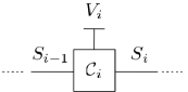
Figure 1: The $q^{s(\mathcal{C})}$-ary graphical model representation of a trellis section.

The hidden (state) variables have alphabet sizes $|T_{i}|\leq s(\mathcal{C})$ and $|T_{i-1}|\leq s(\mathcal{C})$, respectively. The local constraint $\mathcal{C}_{i}$ has length

$$n(\mathcal{C}_{i})=|T_{i}|+|T_{i-1}|+1$$ (13)

and dimension

$$k(\mathcal{C}_{i})=1+\min\left(|T_{i}|,|T_{i-1}|\right)$$ (14)

so that

$$n(\mathcal{C}_{i})-k(\mathcal{C}_{i})=\max\left(|T_{i}|,|T_{i-1}|\right)\leq s(\mathcal{C}).$$ (15)

Lower bounds on $s\left(\mathcal{C}\right)$ do not, however, necessarily extend to $t\left(\mathcal{C}\right)$. For example, the minimal trellis complexity of a length $2^{m}$, dimension $m+1$, binary first-order Reed Muller code is known to be $m$ for $m\geq 3$ [36], whereas the conditionally cycle-free generalized Tanner graphs for these codes described in [40] have a natural interpretation as $2^{m-1}$-ary cycle-free graphical models. The Cut-Set Bound, however, precludes $t(\mathcal{C})$ from being significantly smaller than $s(\mathcal{C})$ [10, 30].

The following lemma concerning minimal tree complexity will be used in the proof of Theorem 3 in Section IV.

Lemma 1

Let $\mathcal{C}$ and $\mathcal{C}^{SPC}$ be linear codes over $\mathbb{F}_{q}$ defined on the index sets $I$ and $J\subseteq I$, respectively, such that $\mathcal{C}^{SPC}$ is a $q$-ary single parity-check code. Define by $\widetilde{\mathcal{C}}$ the intersection of $\mathcal{C}$ and $\mathcal{C}^{SPC}$:

$$\widetilde{\mathcal{C}}=\mathcal{C}\cap\mathcal{C}^{SPC}.$$ (16)

The minimal tree complexity of $\widetilde{\mathcal{C}}$ is upper-bounded by

$$t(\widetilde{\mathcal{C}})\leq t(\mathcal{C})+1.$$ (17)

Proof:

By explicit construction of a $q^{t(\mathcal{C})+1}$-ary graphical model for $\widetilde{\mathcal{C}}$. Let $\mathcal{G}_{\mathcal{C}}$ be some $q^{t(\mathcal{C})}$-ary cycle-free graphical model for $\mathcal{C}$ and let $\mathcal{T}$ be a minimal connected subtree of $\mathcal{G}_{\mathcal{C}}$ containing the set of $|J|$ interface constraints which involve the visible variables in $J$. Denote by $I_{S}(\mathcal{T})\subseteq I_{S}$ and $I_{C}(\mathcal{T})\subseteq I_{C}$ the subset of hidden variables and local constraints, respectively, contained in $\mathcal{T}$. Choose some local constraint vertex $\mathcal{C}_{\Lambda}$, $\Lambda\in I_{C}(\mathcal{T})$, as a root for $\mathcal{T}$. Observe that the choice of $\mathcal{C}_{\Lambda}$, while arbitrary, induces a directionality in $\mathcal{T}$: downstream toward the root vertex or upstream away from the root vertex. For every $S_{i}$, $i\in I_{S}(\mathcal{T})$, denote by $J_{i,\uparrow}\subseteq J$ the subset of visible variables in $J$ which are upstream from that hidden variable edge.

A $q^{t(\mathcal{C})+1}$-ary graphical model for $\widetilde{\mathcal{C}}$ is then constructed from $\mathcal{G}_{\mathcal{C}}$ by updating each hidden variable $S_{i}$, $i\in I_{S}(\mathcal{T})$, to also contain the $q$-ary partial parity of the upstream visible variables in $J_{i,\uparrow}\subseteq J$. The local constraints $\mathcal{C}_{j}$, $j\in I_{C}(\mathcal{T})\setminus\Lambda$, are updated accordingly. Finally, $\mathcal{C}_{\Lambda}$ is updated to enforce the $q$-ary single parity constraint defined by $\mathcal{C}^{SPC}$. This updating procedure increases the alphabet size of each hidden variable $S_{i}$, $i\in I_{S}(\mathcal{T})$, by at most one and adds at most one single parity-check (or repetition) constraint to the definition of each $\mathcal{C}_{j}$, $j\in I_{C}(\mathcal{T})$, and the resulting cycle-free graphical model is thus at most $q^{t(\mathcal{C})+1}$-ary. ∎

The proof of Lemma 1 is detailed further by example in the appendix.

IV The Tradeoff Between Cyclic Topology and Complexity

IV-A The Cut-Set and Square-Root Bounds

Wiberg’s Cut-Set Bound (CSB) [5, 6] is stated below without proof in the language of Section II.

Theorem 1 (Cut-Set Bound)

Let $\mathcal{C}$ be a linear code over $\mathbb{F}_{q}$ defined on the index set $I$. Let $\mathcal{G_{C}}$ be a graphical model for $\mathcal{C}$ containing a cut $\mathcal{X}$ corresponding to the hidden variables $S_{i}$, $i\in I_{S}(\mathcal{X})$, which partitions the index set into $J_{1}\subset I$ and $J_{2}\subset I$. Let the base-$q$ logarithm of the midpoint hidden variable alphabet size of the minimal two-section trellis for $\mathcal{C}$ on the two-section time axis $\left\{J_{1},J_{2}\right\}$ be $s_{\mathcal{X},\min}$. The sum of the hidden variable alphabet sizes corresponding to the cut $\mathcal{X}$ is lower-bounded by

$$\sum_{i\in I_{S}(\mathcal{X})}\left|T_{i}\right|\geq s_{\mathcal{X},\min}.$$ (18)

The CSB provides insight into the tradeoff between cyclic topology and complexity in graphical models for codes and it is natural to explore its power to quantify this tradeoff. Two questions which arise for a given linear code $\mathcal{C}$ over $\mathbb{F}_{q}$ in such an exploration are:

1. For a given complexity $m$, how many cycles must be contained in a $q^{m}$-ary graphical model for $\mathcal{C}$?

2. For a given number of cycles $N$, what is the smallest $m$ such that a $q^{m}$-ary model containing $N$ cycles for $\mathcal{C}$ can exist?

For a fixed cyclic topology, the CSB can be simultaneously applied to all cuts yielding a linear programming lower bound on the hidden variable alphabet sizes [5]. For the special case of a single-cycle graphical model (i.e. a tail-biting trellis), this technique yields a simple solution [28]:

Theorem 2 (Square-Root Bound)

Let $\mathcal{C}$ be a linear code over $\mathbb{F}_{q}$ of even length and let $s_{\operatorname{mid},\min}(\mathcal{C})$ be the base-$q$ logarithm of the minimum possible hidden variable alphabet size of a conventional trellis for $\mathcal{C}$ at its midpoint over all coordinate orderings. The base-$q$ logarithm of the minimum possible hidden variable alphabet size $s_{\operatorname{TB}}(\mathcal{C})$ of a tail-biting trellis for $\mathcal{C}$ is lower-bounded by

$$s_{\operatorname{TB}}(\mathcal{C})\geq s_{\operatorname{mid},\min}(\mathcal{C})/2.$$ (19)

The square-root bound can thus be used to answer the questions posed above for a specific class of single-cycle graphical models. For topologies richer than a single cycle, however, the aforementioned linear programming technique quickly becomes intractable. Specifically, there are

$$2^{n(\mathcal{C})-1}-1$$ (20)

ways to partition a size $n(\mathcal{C})$ visible variable index set into two non-empty, disjoint, subsets. The number of cuts to be considered by the linear programming technique for a given cyclic topology thus grows exponentially with block length and a different minimal two-stage trellis must be constructed in order to bound the size of each of those cuts.

IV-B Tree-Inducing Cuts

Recall that a cut in a graph $\mathcal{G}$ is some subset of the edges $\mathcal{X}\subseteq\mathcal{E}$ the removal of which yields a disconnected graph. A cut is thus defined without regard to the cyclic topology of the disconnected components which remain after its removal. In order to provide a characterization of the tradeoff between cyclic topology and complexity which is more precise than that provided by the CSB alone, this work focuses on a specific type of cut which is defined below. Two useful properties of such cuts are established by Propositions 2 and 3.

Definition 2

Let $\mathcal{G}$ be a connected graph. A tree-inducing cut is some subset of edges $\mathcal{X}_{T}\subseteq\mathcal{E}$ the removal of which yields a tree with precisely two components.

Proposition 2

Let $\mathcal{G}=\left(\mathcal{V},\mathcal{E},\mathcal{H}\right)$ be a connected graph. The size $X_{T}$ of any tree-inducing cut $\mathcal{X}_{T}$ in $\mathcal{G}$ is precisely

$$X_{T}=\left|\mathcal{E}\right|-\left|\mathcal{V}\right|+2.$$ (21)

Proof:

It is well-known that a connected graph is a tree if and only if (cf. [41])

$$\left|\mathcal{E}\right|=\left|\mathcal{V}\right|-1.$$ (22)

Similarly, a graph composed of two cycle-free components satisfies

$$\left|\mathcal{E}\right|=\left|\mathcal{V}\right|-2.$$ (23)

The result then follows from the observation that the size of a tree-inducing cut is the number of edges which must be removed in order to satisfy (23). ∎

Proposition 3

Let $\mathcal{G}$ be a connected graph with tree-inducing cut size $X_{T}$. The number of cycles $N_{\mathcal{G}}$ in $\mathcal{G}$ is lower-bounded by

$$N_{\mathcal{G}}\geq\binom{X_{T}}{2}.$$ (24)

Proof:

Let the removal of a tree-inducing cut $\mathcal{X}_{T}$ in the connected graph $\mathcal{G}$ yield the cycle-free components $\mathcal{G}_{1}$ and $\mathcal{G}_{2}$ and let $e_{i}\neq e_{j}\in\mathcal{X}_{T}$. Since $\mathcal{G}_{1}$ ($\mathcal{G}_{2}$) is a tree, there is a unique path in $\mathcal{G}_{1}$ ($\mathcal{G}_{2}$) connecting $e_{i}$ and $e_{j}$. There is thus a unique cycle in $\mathcal{G}$ corresponding to the edge pair $\{e_{i},e_{j}\}$. There are $\binom{X_{T}}{2}$ such distinct edge pairs which yields the lower bound. Note that this is a lower bound because for certain graphs, there can exist cycles which contain more than two edges from a tree-inducing cut. ∎

IV-C The Tree-Inducing Cut-Set Bound

With tree-inducing cuts defined, the required properties of $q^{m}$-ary graphical models described and Lemma 1 established, the main result concerning the tradeoff between cyclic topology and graphical model complexity can now be stated and proved.

Theorem 3

Let $\mathcal{C}$ be a linear code over $\mathbb{F}_{q}$ defined on the index set $I$ and suppose that $\mathcal{G}_{\mathcal{C}}$ is a $q^{m}$-ary graphical model for $\mathcal{C}$ with tree-inducing cut size $X_{T}$. The minimal tree complexity of $\mathcal{C}$ is upper-bounded by

$$t(\mathcal{C})\leq mX_{T}.$$ (25)

Proof:

By induction on $X_{T}$. Let $X_{T}=1$ and suppose that $e\in\mathcal{X}_{T}$ is the sole edge in some tree-inducing cut $\mathcal{X}_{T}$ in $\mathcal{G}_{\mathcal{C}}$. Since the removal of $e$ partitions $\mathcal{G}_{\mathcal{C}}$ into disconnected cycle-free components, $\mathcal{G}_{\mathcal{C}}$ must be cycle-free and $t(\mathcal{C})\leq m$ by construction.

Now suppose that $X_{T}=x>1$ and let $e\in\mathcal{X}_{T}$ be an edge in some tree-inducing cut $\mathcal{X}_{T}$ in $\mathcal{G}_{\mathcal{C}}$. By the first $q^{m}$-ary graphical model property of Section III-B, $e$ is incident on some internal local constraint $\mathcal{C}_{i}$ satisfying $n(\mathcal{C}_{i})-k(\mathcal{C}_{i})=m^{\prime}\leq m$. Denote by $\mathcal{G}_{\mathcal{C}^{\setminus i}}$ the $q^{m}$-ary graphical model that results when $\mathcal{C}_{i}$ is removed from $\mathcal{G}_{\mathcal{C}}$, and by $\mathcal{C}^{\setminus i}$ the corresponding code over $I$. The tree-inducing cut size of $\mathcal{G}_{\mathcal{C}^{\setminus i}}$ is at most $x-1$ since the removal of $\mathcal{C}_{i}$ from $\mathcal{G}_{\mathcal{C}}$ results in the removal a single vertex and at least two edges. By the induction hypothesis, the minimal tree complexity of $\mathcal{C}^{\setminus i}$ is upper-bounded by

$$t(\mathcal{C}^{\setminus i})\leq m(x-1).$$ (26)

From the discussion of Section III-B, it is clear that $\mathcal{C}_{i}$ can be redefined as $m^{\prime}\leq m$ single parity check equations, $\mathcal{C}_{i}^{(j)}$ for $j\in[1,m^{\prime}]$, over $\mathbb{F}_{q}$ on $I$ such that

$$\mathcal{C}=\mathcal{C}^{\setminus i}\cap\mathcal{C}_{i}^{(1)}\cap\cdots\cap\mathcal{C}_{i}^{(m^{\prime})}.$$ (27)

It follows from Lemma 1 that

$$t(\mathcal{C})\leq t(\mathcal{C}^{\setminus i})+m^{\prime}\leq mx$$ (28)

completing the proof. ∎

An immediate corollary to Theorem 3 results when Proposition 3 is applied in conjunction with the main result:

Corollary 1

Let $\mathcal{C}$ be a linear code over $\mathbb{F}_{q}$ with minimal tree complexity $t(\mathcal{C})$. The number of cycles $N_{m}$ in any $q^{m}$-ary graphical model for $\mathcal{C}$ is lower-bounded by

$$N_{m}\geq\binom{\left\lfloor t(\mathcal{C})/m\right\rfloor}{2}.$$ (29)

IV-D Interpretation of the TI-CSB

Provided $t(\mathcal{C})$ is known or can be lower-bounded, the tree-inducing cut-set bound (TI-CSB) (and more specifically Corollary 1) can be used to answer the questions posed in Section IV-A. The TI-CSB is further discussed below.

IV-D1 The TI-CSB and the CSB

On the surface, the TI-CSB and the CSB are similar in statement; however, there are three important differences between the two. First, the CSB does not explicitly address the complexity of the local constraints on either side of a given cut. Forney provided a number of illustrative examples in [30] that stress the importance of characterizing graphical model complexity in terms of both hidden variable size and local constraint complexity. Second, the CSB does not explicitly address the cyclic topology of the graphical model that results when the edges in a cut are removed. The removal of a tree-inducing cut results in two cycle-free disconnected components and the size of a tree-inducing cut can thus be used to make statements about the complexity of optimal SISO decoding using variable conditioning in a cyclic graphical model (cf. [10, 40, 42, 43, 44, 45]). Finally, and most fundamentally, the TI-CSB addresses the aforementioned intractability of applying the CSB to graphical models with rich cyclic topologies.

IV-D2 The TI-CSB and the Square-Root Bound

Theorem 3 can be used to make a statement similar to Theorem 2 which is valid for all graphical models containing a single cycle.

Corollary 2

Let $\mathcal{C}$ be a linear code over $\mathbb{F}_{q}$ with minimal tree complexity $t(\mathcal{C})$ and let $m_{1}$ be the smallest integer such that there exists a $q^{m_{1}}$-ary graphical model for $\mathcal{C}$ which contains at most one cycle. Then

$$m_{1}\geq t(\mathcal{C})/2.$$ (30)

More generally, Theorem 3 can be used to establish the following generalization of the square-root bound to graphical models with arbitrary cyclic topologies.

Corollary 3

Let $\mathcal{C}$ be a linear code over $\mathbb{F}_{q}$ with minimal tree complexity $t(\mathcal{C})$ and let $m_{\binom{r}{2}}$ be the smallest integer such that there exists a $q^{m_{\binom{r}{2}}}$-ary graphical model for $\mathcal{C}$ which contains at most $\binom{r}{2}$ cycles. Then

$$m_{\binom{r}{2}}\geq t(\mathcal{C})/r.$$ (31)

A linear interpretation of the logarithmic complexity statement of Corollary 3 yields the desired generalization of the square-root bound: an $r^{th}$-root complexity reduction with respect to the minimal tree complexity requires the introduction of at least $r(r-1)/2$ cycles.

There are few known examples of classical linear block codes which meet the square-root bound with equality. Shany and Be’ery proved that many RM codes cannot meet this bound under any bit ordering [46]. There does, however, exist a tail-biting trellis for the extended binary Golay code $\mathcal{C}_{G}$ which meets the square-root bound with equality so that [28]

$$s_{\operatorname{mid},\min}(\mathcal{C}_{G})=8\quad\mbox{and}\quad s_{\operatorname{TB}}(\mathcal{C}_{G})=4.$$ (32)

Given that this tail-biting trellis is a $2^{4}$-ary single cycle graphical model for $\mathcal{C}_{G}$, the minimal tree complexity of the the extended binary Golay code can be upper-bounded by Corollary 2 as

$$t(\mathcal{C}_{G})\leq 8.$$ (33)

Note that the minimal bit-level conventional trellis for $\mathcal{C}_{G}$ contains (non-central) state variables with alphabet size $512$ and is thus a $2^{9}$-ary graphical model [35]. The proof of Lemma 1 provides a recipe for the construction of a $2^{8}$-ary cycle-free graphical model for $\mathcal{C}_{G}$ from its tail-biting trellis. It remains open as to where the minimal tree complexity of $\mathcal{C}_{G}$ is precisely $8$, however.

IV-D3 Aymptotics of the TI-CSB

Denote by $N_{m}$ the minimum number of cycles in any $q^{m}$-ary graphical model for a linear code $\mathcal{C}$ over $\mathbb{F}_{q}$ with minimal tree complexity $t(\mathcal{C})$. For large values of $t(\mathcal{C})/m$, the lower bound on $N_{m}$ established by Corollary 1 becomes

$$N_{m}\geq\binom{\left\lfloor t(\mathcal{C})/m\right\rfloor}{2}\approx\frac{t(\mathcal{C})^{2}}{2m^{2}}.$$ (34)

The ratio of the minimal complexity of a cycle-free model for $\mathcal{C}$ to that of an $q^{m}$-ary graphical model is thus upper-bounded by

$$\frac{q^{t(\mathcal{C})}}{q^{m}}\lessapprox q^{2m\sqrt{N_{m}}}.$$ (35)

In order to further explore the asymptotics of the tree-inducing cut-set bound, consider a code of particular practical interest: the binary image $\mathcal{C}_{RS|\mathbb{F}_{2}}$ of the $[255,223,33]$ Reed-Solomon code $\mathcal{C}_{RS}$. Since $\mathcal{C}_{RS}$ is maximum distance separable, a reasonable estimate for the minimal tree complexity of this code is obtained from Wolf’s bound [47]

$$t(\mathcal{C}_{RS|\mathbb{F}_{2}})\approx 8(n(\mathcal{C}_{RS})-k(\mathcal{C}_{RS}))=256.$$ (36)

Figure 2 plots $N_{m}$ as a function of $m$ for $\mathcal{C}_{RS|\mathbb{F}_{2}}$ assuming (36). Note that since the complexity of the decoding algorithms implied by $2^{m}$-ary graphical models grow roughly as $2^{m}$, $\log m$ is roughly a $\log\log$ decoding complexity measure.

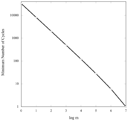
Figure 2: Minimum number of cycles required for $2^{m}$-ary graphical models of the binary image of the $[255,223,33]$ Reed-Solomon code.

IV-D4 On Complexity Measures

Much as there are many valid complexity measures for conventional trellises, there are many reasonable metrics for the measurement of cyclic graphical model complexity. While there exists a unique minimal trellis for any linear block code which simultaneously minimizes all reasonable measures of complexity [48], even for the class cyclic graphical models with the most basic cyclic topology - tail-biting trellises - minimal models are not unique [29]. The complexity measure introduced by this work was motivated by the desire to have a metric which simultaneously captures hidden variable complexity and local constraint complexity thus disallowing local constraints from “hiding” complexity. There are many conceivable measures of local constraint complexity: one could upper-bound the state complexity of the local constraints or even their minimal tree complexity (thus defining minimal tree complexity recursively). The local constraint complexity measure used in this work is essentially Wolf’s bound [47] and is thus a potentially conservative upper bound on any reasonable measure of local constraint decoding complexity.

V Graphical Model Transformation

Let $\mathcal{G_{C}}$ be a graphical model for the linear code $\mathcal{C}$ over $\mathbb{F}_{q}$. This work introduces eight basic graphical model operations the application of which to $\mathcal{G_{C}}$ results in a new graphical model for $\mathcal{C}$:

• The merging of two local constraints $\mathcal{C}_{i_{1}}$ and $\mathcal{C}_{i_{2}}$ into the new local constraint $\mathcal{C}_{i}$ which satisfies

  $$\mathcal{C}_{i}=\mathcal{C}_{i_{1}}\cap\;\mathcal{C}_{i_{2}}.$$ (37)

• The splitting of a local constraint $\mathcal{C}_{j}$ into two new local constraints $\mathcal{C}_{j_{1}}$ and $\mathcal{C}_{j_{2}}$ which satisfy

  $$\mathcal{C}_{j_{1}}\cap\;\mathcal{C}_{j_{2}}=\mathcal{C}_{j}.$$ (38)

• The insertion/removal of a degree-$2$ repetition constraint.

• The insertion/removal of a trival length $0$, dimension $0$ local constraint.

• The insertion/removal of an isolated partial parity-check constraint.

Note that some of these operations have been introduced implicitly in this work and others already. For example, the proof of the local constraint involvement property of $q^{m}$-ary graphical models presented in Section III-B utilizes degree-$2$ repetition constraint insertion. Local constraint merging has been considered by a number of authors under the rubric of clustering (e.g. [9, 10]). This work introduces the term merging specifically so that it can be contrasted with its inverse operation: splitting. Detailed definitions of each of the eight basic graphical model operations are given in the appendix. In this section, it is shown that these basic operations span the entire space of graphical models for $\mathcal{C}$.

Theorem 4

Let $\mathcal{G_{C}}$ and $\widetilde{\mathcal{G}}_{\mathcal{C}}$ be two graphical models for the linear code $\mathcal{C}$ over $\mathbb{F}_{q}$. Then $\mathcal{G_{C}}$ can be transformed into $\widetilde{\mathcal{G}}_{\mathcal{C}}$ via the application of a finite number of basic graphical model operations.

Proof:

Define the following four sub-transformations which can be used to transform $\mathcal{G}_{\mathcal{C}}$ into a Tanner graph $\mathcal{G}_{\mathcal{C}}^{T}$:

1. The transformation of $\mathcal{G}_{\mathcal{C}}$ into a $q$-ary model $\mathcal{G}_{\mathcal{C}}^{q}$.

2. The transformation of $\mathcal{G}_{\mathcal{C}}^{q}$ into a (possibly) redundant generalized Tanner graph $\mathcal{G}_{\mathcal{C}}^{r}$.

3. The transformation of $\mathcal{G}_{\mathcal{C}}^{r}$ into a non-redundant generalized Tanner graph $\mathcal{G}_{\mathcal{C}}^{g}$.

4. The transformation of $\mathcal{G}_{\mathcal{C}}^{g}$ into a Tanner graph $\mathcal{G}_{\mathcal{C}}^{T}$.

Since each basic graphical model operation has an inverse, $\mathcal{G}_{\mathcal{C}}^{T}$ can be transformed into $\mathcal{G}_{\mathcal{C}}$ by inverting each of the four sub-transformations. In order to prove that $\mathcal{G}_{\mathcal{C}}$ can be transformed into $\widetilde{\mathcal{G}}_{\mathcal{C}}$ via the application of a finite number of basic graphical model operations, it suffices to show that each of the four sub-transformations requires a finite number of operations and that the transformation of the Tanner graph $\mathcal{G}_{\mathcal{C}}^{T}$ into a Tanner graph $\widetilde{\mathcal{G}}_{\mathcal{C}}^{T}$ corresponding to $\widetilde{\mathcal{G}}_{\mathcal{C}}$ requires a finite number of operations. This proof summary is illustrated in Figure 3.

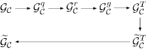
Figure 3: The transformation of $\mathcal{G}_{\mathcal{C}}$ into $\widetilde{\mathcal{G}}_{\mathcal{C}}$ via five sub-transformations.

That each of the five sub-transformations from $\mathcal{G}_{\mathcal{C}}$ to $\widetilde{\mathcal{G}}_{\mathcal{C}}^{T}$ illustrated in Figure 3 requires only a finite number of basic graphical model operations is proved below.

V-1 $\mathcal{G}_{\mathcal{C}}\rightarrow\mathcal{G}_{\mathcal{C}}^{q}$

The graphical model $\mathcal{G}_{\mathcal{C}}$ is transformed into the $q$-ary model $\mathcal{G}_{\mathcal{C}}^{q}$ as follows. Each local constraint $\mathcal{C}_{i}$ in $\mathcal{G}_{\mathcal{C}}$ is split into the $n(\mathcal{C}_{i})-k(\mathcal{C}_{i})$ $q$-ary single parity-check constraints which define it. A degree-$2$ repetition constraint is then inserted into every hidden variable with alphabet index set size $m>1$ and these repetition constraints are then each split into $m$ $q$-ary repetition constraints as illustrated in Figure 4. Each local constraint $\mathcal{C}_{j}$ in the resulting graphical model satisfies $n(\mathcal{C}_{j})-k(\mathcal{C}_{j})=1$. Similarly, each hidden variable $S_{j}$ in the resulting graphical model satisfies $|T_{j}|=1$.

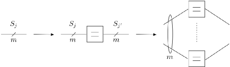
Figure 4: Transformation of the $q^{m}$-ary hidden variable $S_{j}$ into $q$-ary hidden variables.

V-2 $\mathcal{G}_{\mathcal{C}}^{q}\rightarrow\mathcal{G}_{\mathcal{C}}^{r}$

A (possibly redundant) generalized Tanner graph is simply a bipartite $q$-ary graphical model with one vertex class corresponding to repetition constraints and one to single parity-check constraints in which visible variables are incident only on repetition constraints. By appropriately inserting degree-$2$ repetition constraints, the $q$-ary model $\mathcal{G}_{\mathcal{C}}^{q}$ can be transformed into $\mathcal{G}_{\mathcal{C}}^{r}$.

V-3 $\mathcal{G}_{\mathcal{C}}^{r}\rightarrow\mathcal{G}_{\mathcal{C}}^{g}$

Let the generalized Tanner graph $\mathcal{G}_{\mathcal{C}}^{r}$ correspond to an $r_{H}\times n(\mathcal{C})+g$ redundant parity-check matrix $H^{(r,g)}_{\mathcal{C}}$ for a degree-$g$ generalized extension of $\mathcal{C}$ with rank

$$\operatorname{rank}(H^{(r,g)}_{\mathcal{C}})=n(\mathcal{C})-k(\mathcal{C})+g.$$ (39)

A finite number of row operations can be applied to $H^{(r,g)}_{\mathcal{C}}$ resulting in a new parity-check matrix the last $r_{H}-\operatorname{rank}(H^{(r,g)}_{\mathcal{C}})$ rows of which are all zero. Similarly, a finite number of basic operations can be applied to $\mathcal{G}_{\mathcal{C}}^{r}$ resulting in a generalized Tanner graph containing $r_{H}-\operatorname{rank}(H^{(r,g)}_{\mathcal{C}})$ trivial constraints which can then be removed to yield $\mathcal{G}_{\mathcal{C}}^{g}$. Specifically, consider the row operation on $H^{(r,g)}_{\mathcal{C}}$ which replaces a row $\boldsymbol{h}_{i}$ by

$$\widetilde{\boldsymbol{h}}_{i}=\boldsymbol{h}_{i}+\beta_{j}\boldsymbol{h}_{j}$$ (40)

where $\beta_{j}\in\mathbb{F}_{q}$. The graphical model transformation corresponding to this row operation first merges the $q$-ary single parity-check constraints $\mathcal{C}_{i}$ and $\mathcal{C}_{j}$ (which correspond to rows $\boldsymbol{h}_{i}$ and $\boldsymbol{h}_{j}$, respectively) and then splits the resulting check into the constraints $\widetilde{\mathcal{C}_{i}}$ and $\mathcal{C}_{j}$ (which correspond to rows $\widetilde{\boldsymbol{h}}_{i}$ and $\boldsymbol{h}_{j}$, respectively). Note that this procedure is valid since

$$\mathcal{C}_{i}\cap\mathcal{C}_{j}=\widetilde{\mathcal{C}}_{i}\cap\mathcal{C}_{j}.$$ (41)

V-4 $\mathcal{G}_{\mathcal{C}}^{g}\rightarrow\mathcal{G}_{\mathcal{C}}^{T}$

Let the degree-$g$ generalized Tanner graph $\mathcal{G}_{\mathcal{C}}^{g}$ correspond to an $n(\mathcal{C})-k(\mathcal{C})+g\times n(\mathcal{C})+g$ parity-check matrix $H_{\mathcal{C}}^{(g)}$. A degree-$(g-1)$ generalized Tanner graph $\mathcal{G}_{\mathcal{C}}^{g-1}$ is obtained from $\mathcal{G}_{\mathcal{C}}^{g}$ as follows. Denote by $\widehat{H}_{\mathcal{C}}^{(g)}$ the parity-check matrix for the degree-$g$ generalized extension defined by $H_{\mathcal{C}}^{(g)}$ which is systematic in the position corresponding to the $g$-th partial parity symbol. Since a finite number of row operations can be applied to $H_{\mathcal{C}}^{(g)}$ to yield $\widehat{H}_{\mathcal{C}}^{(g)}$, a finite number of local constraint merge and split operations can be be applied to $\mathcal{G}_{\mathcal{C}}^{g}$ to yield the corresponding generalized Tanner graph $\widehat{\mathcal{G}}_{\mathcal{C}}^{g}$. Removing the now isolated partial-parity check constraint corresponding to the $g$-th partial parity symbol in $\widehat{\mathcal{G}}_{\mathcal{C}}^{g}$ yields the desired degree-$(g-1)$ generalized Tanner graph $\mathcal{G}_{\mathcal{C}}^{g-1}$. By repeatedly applying this procedure, all partial parity symbols can be removed from $\mathcal{G}_{\mathcal{C}}^{g}$ resulting in $\mathcal{G}_{\mathcal{C}}^{T}$.

V-5 $\mathcal{G}_{\mathcal{C}}^{T}\rightarrow\widetilde{\mathcal{G}}_{\mathcal{C}}^{T}$

Let the Tanner graphs $\mathcal{G}_{\mathcal{C}}^{T}$ and $\widetilde{\mathcal{G}}_{\mathcal{C}}^{T}$ correspond to the parity-check matrices $H_{\mathcal{C}}$ and $\widetilde{H}_{\mathcal{C}}$, respectively. Since $H_{\mathcal{C}}$ can be transformed into $\widetilde{H}_{\mathcal{C}}$ via a finite number of row operations, $\mathcal{G}_{\mathcal{C}}^{T}$ can be similarly transformed into $\widetilde{\mathcal{G}}_{\mathcal{C}}^{T}$ via the application of a finite number of local constraint merge and split operations. ∎

VI Graphical Model Extraction via Transformation

The set of basic model operations introduced in the previous section enables the space of all graphical models for a given code $\mathcal{C}$ to be searched, thus allowing for model extraction to be expressed as an optimization problem. The challenges of defining extraction as optimization are twofold. First, a cost measure on the space of graphical models must be found which is simultaneously meaningful in some real sense (e.g. highly correlated with decoding performance) and computationally tractable. Second, given that discrete optimization problems are in general very hard, heuristics for extraction must be found. In this section, heuristics are investigated for the extraction of graphical models for binary linear block codes from an initial Tanner graph. The cost measures considered are functions of the short cycle structure of graphical models. The use of such cost measures is motivated first by empirical evidence concerning the detrimental effect of short cycles on decoding performance (cf. [6, 10, 11, 12, 13, 14, 15, 16]) and second by the existence of an efficient algorithm for counting short cycles in bipartite graphs [16]. Simulation results for the models extracted via these heuristics for a number of extended BCH codes are presented and discussed in Section VI-D.

VI-A A Greedy Heuristic for Tanner Graph Extraction

The Tanner graphs corresponding to many linear block codes of practical interest necessarily contain many short cycles [26]. Suppose that any Tanner graph for a given code $\mathcal{C}$ must have girth at least $g_{\min}(\mathcal{C})$; an interesting problem is the extraction of a Tanner graph for $\mathcal{C}$ containing the smallest number of $g_{\min}(\mathcal{C})$-cycles. The extraction of such Tanner graphs is especially useful in the context of ad-hoc decoding algorithms which utilize Tanner graphs such as Jiang and Narayanan’s stochastic shifting based iterative decoding algorithm for cyclic codes [49] and the random redundant iterative decoding algorithm presented in [50].

Algorithm 1 performs a greedy search for a Tanner graph for $\mathcal{C}$ with girth $g_{\min}(\mathcal{C})$ and the smallest number of $g_{\min}(\mathcal{C})$-cycles starting with an initial Tanner graph $\operatorname{TG}(H_{\mathcal{C}})$ which corresponds to some binary parity-check matrix $H_{\mathcal{C}}$. Define an $(i,j)$-row operation as the replacement of row $\boldsymbol{h}_{j}$ in $H_{\mathcal{C}}$ by the binary sum of rows $\boldsymbol{h}_{i}$ and $\boldsymbol{h}_{j}$. As detailed in the proof of Theorem 4, if $\mathcal{C}_{i}$ and $\mathcal{C}_{j}$ are the single parity-check constraints in $\operatorname{TG}(H_{\mathcal{C}})$ corresponding to $\boldsymbol{h}_{i}$ and $\boldsymbol{h}_{j}$, respectively, then an $(i,j)$-row operation in $H_{\mathcal{C}}$ is equivalent to merging $\mathcal{C}_{i}$ and $\mathcal{C}_{j}$ to form a new constraint $\mathcal{C}_{i,j}=\mathcal{C}_{i}\cap\mathcal{C}_{j}$ and then splitting $\mathcal{C}_{i,j}$ into $\mathcal{C}_{i}$ and $\widetilde{\mathcal{C}}_{j}$ (where $\widetilde{\mathcal{C}}_{j}$ enforces the binary sum of rows $\boldsymbol{h}_{i}$ and $\boldsymbol{h}_{j}$). Algorithm 1 iteratively finds the rows $\boldsymbol{h}_{i}$ and $\boldsymbol{h}_{j}$ in $H_{\mathcal{C}}$ with corresponding $(i,j)$-row operation that results in the largest short cycle reduction in $\operatorname{TG}(H_{\mathcal{C}})$ at every step. This greedy search continues until there are no more row operations that improve the short cycle structure of $\operatorname{TG}(H_{\mathcal{C}})$.

Input: $r_{H}\times n(\mathcal{C})$ binary parity-check matrix $H_{\mathcal{C}}$.

Output: $r_{H}\times n(\mathcal{C})$ binary parity-check matrix $H_{\mathcal{C}}^{\prime}$.

$H_{\mathcal{C}}^{\prime}\leftarrow H_{\mathcal{C}}$; $i^{\star}\leftarrow-1$; $j^{\star}\leftarrow-1$; $g^{\star}\leftarrow$ girth of $\operatorname{TG}\left(H^{\prime}_{\mathcal{C}}\right)$;

$N_{g^{\star}}^{\star}\leftarrow$ number of $g^{\star}$-cycles in $\operatorname{TG}\left(H_{\mathcal{C}}^{\prime}\right)$;

$N_{g^{\star}+2}^{\star}\leftarrow$ number of $g^{\star}+2$-cycles in $\operatorname{TG}\left(H_{\mathcal{C}}^{\prime}\right)$;

repeat  if $i^{\star}\neq j^{\star}$ then Replace row $\boldsymbol{h}_{j^{\star}}$ in $H_{\mathcal{C}}^{\prime}$ with binary sum of rows $\boldsymbol{h}_{i^{\star}}$ and $\boldsymbol{h}_{j^{\star}}$;

$i^{\star}\leftarrow-1$; $j^{\star}\leftarrow-1$;

for $i,j=0,\ldots,r_{H}-1$, $i\neq j$ do  Replace row $\boldsymbol{h}_{j}$ in $H_{\mathcal{C}}^{\prime}$ with binary sum of rows $\boldsymbol{h}_{i}$ and $\boldsymbol{h}_{j}$;

$g\leftarrow$ girth of $\operatorname{TG}\left(H_{\mathcal{C}}^{\prime}\right)$;

$N_{g}\leftarrow$ number of $g$-cycles in $\operatorname{TG}\left(H_{\mathcal{C}}^{\prime}\right)$;

$N_{g+2}\leftarrow$ number of $g+2$-cycles in $\operatorname{TG}\left(H_{\mathcal{C}}^{\prime}\right)$;

if $g>g^{\star}$ then  $g^{\star}\leftarrow g$; $i^{\star}\leftarrow i$; $j^{\star}\leftarrow j$; $N_{g}^{\star}\leftarrow N_{g}$; $N_{g+2}^{\star}\leftarrow N_{g+2}$;

end else if $g=g^{\star}$ AND $N_{g}<N_{g}^{\star}$ then $i^{\star}\leftarrow i$; $j^{\star}\leftarrow j$; $N_{g}^{\star}\leftarrow N_{g}$; $N_{g+2}^{\star}\leftarrow N_{g+2}$;

else if $g=g^{\star}$ AND $N_{g}=N_{g}^{\star}$ then  if $N_{g+2}<N_{g+2}^{\star}$ then $i^{\star}\leftarrow i$; $j^{\star}\leftarrow j$; $N_{g+2}^{\star}\leftarrow N_{g+2}$;

end Undo row replacement;

end until $i^{\star}=-1$ & $j^{\star}=-1$;

return $H_{\mathcal{C}}^{\prime}$

 

Algorithm 1 Greedy heuristic for the reduction of short cycles in Tanner graphs for binary codes.

VI-B A Greedy Heuristic for Generalized Tanner Graph Extraction

A number of authors have studied the extraction of generalized Tanner graphs (GTGs) of codes for which $g_{\min}(\mathcal{C})=4$ with a particular focus on models which are $4$-cycle-free and which correspond to generalized code extensions of minimal degree [51, 52]. Minimal degree extensions are sought because no information is available to the decoder about the partial parity symbols in a generalized Tanner graph and the introduction of too many such symbols has been observed empirically to adversely affect decoding performance [52].

Generalized Tanner graph extraction algorithms proceed via the insertion of partial parity symbols, an operation which is most readily described as a parity-check matrix manipulation. Following the notation introduced in Section II-F, suppose that a partial parity on the coordinates indexed by

$$J\subseteq I\cup\left\{p_{1},p_{2},\ldots,p_{g}\right\}$$ (42)

is to be introduced to a GTG for $\mathcal{C}$ corresponding to a degree-$g$ generalized extension $\widetilde{\mathcal{C}}$ with parity-check matrix $H_{\widetilde{\mathcal{C}}}$. A row $\boldsymbol{h}_{p}$ is first appended to $H_{\widetilde{\mathcal{C}}}$ with a $1$ in the positions corresponding to coordinates indexed by $J$ and a $0$ in the other positions. A column is then appended to $H_{\widetilde{\mathcal{C}}}$ with a $1$ only in the position corresponding to $\boldsymbol{h}_{p}$. The resulting parity-check matrix $H_{\widehat{\mathcal{C}}}$ describes a degree-$g+1$ generalized extension $\widehat{\mathcal{C}}$. Every row $\boldsymbol{h}_{i}\neq\boldsymbol{h}_{p}$ in $H_{\widehat{\mathcal{C}}}$ which contains a $1$ in all of the positions corresponding to coordinates indexed by $J$ is then replaced by the binary sum of $\boldsymbol{h}_{i}$ and $\boldsymbol{h}_{p}$. Suppose that there are $r(J)$ such rows. It is readily verified that the tree-inducing cut size $\widehat{X}_{T}$ of the GTG that results from this insertion is related to that of the initial GTG, $\widetilde{X}_{T}$, by

$$\Delta X_{T}=\widetilde{X}_{T}-\widehat{X}_{T}=(|J|-1)(r(J)-1).$$ (43)

Algorithm 3 performs a greedy search for a $4$-cycle-free generalized Tanner graph for $\mathcal{C}$ with the smallest number of inserted partial parity symbols starting with an initial Tanner graph $\operatorname{TG}(H_{\mathcal{C}})$ which corresponds to some binary parity-check matrix $H_{\mathcal{C}}$. Algorithm 3 iteratively finds the symbol subsets that result in the largest tree-inducing cut size reduction and then introduces the partial parity symbol corresponding to one of those subsets. At each step, Algorithm 3 uses Algorithm 2 to generate a candidate list of partial parity symbols to insert and chooses from that list the symbol which reduces the most short cycles when inserted. This greedy procedure continues until the generalized Tanner graph contains no $4$-cycles.

Algorithm 3 is closely related to the GTG extraction heuristics proposed by Sankaranarayanan and Vasić in [51] and Kumar and Milenkovic in [52] (henceforth referred to as the SV and KM heuristics, respectively). It is readily shown that Algorithm 3 is guaranteed to terminate using the proof technique of [51]. The SV heuristic considers only the insertion of partial parity symbols corresponding to coordinate index sets of size 2 (i.e. $|J|=2$). The KM heuristic considers only the insertion of partial parity symbols corresponding to coordinate index sets satisfying $r(J)=2$. Algorithm 2, however, considers all coordinate index sets satisfying $|J|=2,3,4$ and $r(J)=2,3,4$ and then uses (43) to evaluate which of these coordinate sets results in the largest tree-inducing cut size reduction. Algorithm 3 is thus able to extract GTGs corresponding to generalized extensions of smaller degree than the SV and KM heuristics. In order to illustrate this observation, the degrees of the generalized code extensions that result when the SV, KM and proposed (HC) heuristics are applied to parity-check matrices for three codes are provided in Table I. Figure 5 compares the performance of the three extracted GTG decoding algorithms for the $[31,21,5]$ BCH code in order to illustrate the efficacy of extracting GTGs corresponding to extensions of smallest possible degree.

Code	SV	KM	HC
$[23,12,7]$ Golay	$18$	$11$	$10$
$[31,21,5]$ BCH	$47$	$19$	$12$
$[63,30,13]$ BCH	$264$	$121$	$69$

TABLE I: Generalized code extension degrees corresponding to the $4$-cycle-free GTGs obtained via the SV, KM, and HC heuristics.

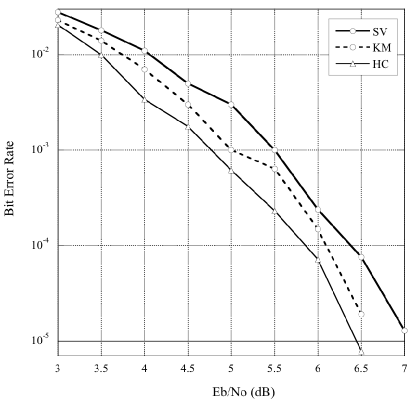
Figure 5: Bit error rate performance of three GTG decoding algorithms for the $[31,21,5]$ BCH code. One-hundred iterations of a flooding schedule were performed. Binary antipodal signaling over an AWGN channel is assumed.

Input: Binary generalized parity-check matrix $H_{\widetilde{\mathcal{C}}}$.

Output: List $\mathcal{S}$ of best partial parity symbols sets.

$\mathcal{S}\leftarrow\emptyset$; $\Delta X_{T}^{\star}\leftarrow 0$;

// Consider pairs of columns of $H_{\widetilde{\mathcal{C}}}$.

$J_{2}\leftarrow$ coordinate pair that maximizes $r(J_{2})$;

Append $J_{2}$ to $\mathcal{S}$; $\Delta X_{T}^{\star}\leftarrow r(J_{2})-1$;

// Consider $3$-tuples of columns of $H_{\widetilde{\mathcal{C}}}$.

$J_{3}\leftarrow$ coordinate $3$-tuple that maximizes $r(J_{3})$;

if $2(r(J_{3})-1)>\Delta X_{T}^{\star}$ then  $\mathcal{S}\leftarrow\emptyset$; Append $J_{3}$ to $\mathcal{S}$; $\Delta X_{T}^{\star}\leftarrow 2(r(J_{3})-1)$;

end else if $2(r(J_{3})-1)=\Delta X_{T}^{\star}$ then Append $J_{3}$ to $\mathcal{S}$;

// Consider $4$-tuples of columns of $H_{\widetilde{\mathcal{C}}}$.

$J_{4}\leftarrow$ coordinate $4$-tuple that maximizes $r(J_{4})$;

if $3(r(J_{4})-1)>\Delta X_{T}^{\star}$ then  $\mathcal{S}\leftarrow\emptyset$; Append $J_{4}$ to $\mathcal{S}$; $\Delta X_{T}^{\star}\leftarrow 3(r(J_{4})-1)$;

end else if $3(r(J_{4})-1)=\Delta X_{T}^{\star}$ then Append $J_{4}$ to $\mathcal{S}$;

// Consider pairs of rows of $H_{\widetilde{\mathcal{C}}}$.

$J_{i}\leftarrow$ largest coordinate subset such that $r(J_{i})=2$;

if $|J_{i}|-1>\Delta X_{T}^{\star}$ then  $\mathcal{S}\leftarrow\emptyset$; Append $J_{i}$ to $\mathcal{S}$; $\Delta X_{T}^{\star}\leftarrow|J_{i}|-1$;

end else if $|J_{i}|-1=\Delta X_{T}^{\star}$ then Append $J_{i}$ to $\mathcal{S}$;

// Consider $3$-tuples of rows of $H_{\widetilde{\mathcal{C}}}$.

$J_{j}\leftarrow$ largest coordinate subset such that $r(J_{j})=3$;

if $2(|J_{j}|-1)>\Delta X_{T}^{\star}$ then  $\mathcal{S}\leftarrow\emptyset$; Append $J_{j}$ to $\mathcal{S}$; $\Delta X_{T}^{\star}\leftarrow 2(|J_{j}|-1)$;

end else if $2(|J_{j}|-1)=\Delta X_{T}^{\star}$ then Append $J_{j}$ to $\mathcal{S}$;

// Consider $4$-tuples of rows of $H_{\widetilde{\mathcal{C}}}$.

$J_{k}\leftarrow$ largest coordinate subset such that $r(J_{k})=4$;

if $3(|J_{k}|-1)>\Delta X_{T}^{\star}$ then  $\mathcal{S}\leftarrow\emptyset$; Append $J_{k}$ to $\mathcal{S}$; $\Delta X_{T}^{\star}\leftarrow 3(|J_{k}|-1)$;

end else if $3(|J_{k}|-1)=\Delta X_{T}^{\star}$ then Append $J_{k}$ to $\mathcal{S}$;

return $\mathcal{S}$

 

Algorithm 2 Heuristic for generating candidate partial parity symbols.

Input: Binary parity-check matrix $H_{\mathcal{C}}$.

Output: Binary generalized parity-check matrix $H_{\widetilde{\mathcal{C}}}$.

$H_{\widetilde{\mathcal{C}}}\leftarrow H_{\mathcal{C}}$;

while $\operatorname{GTG}(H_{\widetilde{\mathcal{C}}})$ contains $4$-cycles do  $\mathcal{S}\leftarrow$ set of candidate partial parity symbol

      subsets from Algorithm 2;

$J^{\star}\leftarrow$ subset in $\mathcal{S}$ the insertion of which reduces

       the most $4$–cycles in $\operatorname{GTG}(H_{\widetilde{\mathcal{C}}})$;

Insert symbol corresponding to $J^{\star}$ in $H_{\widetilde{\mathcal{C}}}$;

end return $H_{\widetilde{\mathcal{C}}}$

 

Algorithm 3 Greedy heuristic for the removal of $4$-cycles in binary generalized Tanner graphs.

VI-C A Greedy Heuristic for $2^{m}$-ary Model Extraction

For most codes, the decoding algorithms implied by generalized Tanner graphs exhibit only modest gains with respect to those implied by Tanner graphs, if any, thus motivating the search for more complex graphical models. Algorithm 4 iteratively applies the constraint merging operation in order to obtain a $2^{m^{\star}}$-ary graphical model from an initial Tanner graph $\operatorname{TG}(H_{\mathcal{C}})$ for some prescribed maximum complexity $m^{\star}$. At each step, Algorithm 4 determines the pair of local constraints $\mathcal{C}_{i}$ and $\mathcal{C}_{j}$ which when merged reduces the most short cycles without violating the maximum complexity constraint $m^{\star}$. In order to ensure that that the efficient cycle counting algorithm of [16] can be utilized, only pairs of checks which are both internal or both interface are merged at each step. Since the initial Tanner graph is bipartite with vertex classes corresponding to interface (repetition) and internal (single parity-check) constraints, the graphical models that result from every such local constraint merge operations are similarly bipartite.

Input: Tanner graph $\operatorname{TG}(H_{\mathcal{C}})$. Max. complexity $m^{\star}$.

Output: $2^{m^{\star}}$-ary graphical model $\operatorname{GM}$ for $\mathcal{C}$.

$\operatorname{GM}\leftarrow\operatorname{TG}(H_{\mathcal{C}})$;

repeat  $(\mathcal{C}_{i},\mathcal{C}_{j})\leftarrow$ pair of incident or internal constraints

             the removal of which removes the most

             $4$-cycles from $\operatorname{GM}$ while not violating

             the $2^{m^{\star}}$-ary complexity constraint;

Merge local constraints $\mathcal{C}_{i}$ and $\mathcal{C}_{j}$ in $\operatorname{GM}$;

until No allowed $4$-cycle reducing merge operations remain;

return $\operatorname{GM}$

 

Algorithm 4 Greedy heuristic for the extraction of $2^{m}$-ary graphical models.

VI-D Simulation Results

The proposed extraction heuristics were applied to two extended BCH codes with parameters $[32,21,6]$ and $[64,51,6]$, respectively. In both Figures 6 and 7 the performance of a number of suboptimal SISO decoding algorithms for these codes is compared to algebraic hard-in hard-out (HIHO) decoding and optimal trellis SISO decoding. Binary antipodal signaling over AWGN channels is assumed throughout.

Initial parity-check matrices $H$ were formed by extending cyclic parity-check matrices for the respective $[31,21,5]$ and $[63,51,5]$ BCH codes [31]. These initial parity-check matrices were used as inputs to Algorithm 1, yielding the parity-check matrices $H^{\prime}$, which in turn were used as inputs to Algorithm 3, yielding $4$-cycle-free generalized Tanner graphs. The suboptimal decoding algorithms implied by these graphical models are labeled $\operatorname{TG}(H)$, $\operatorname{TG}(H^{\prime})$, and $\operatorname{GTG}(H^{\prime})$, respectively. The generalized Tanner graphs extracted for the $[32,21,6]$ and $[64,51,6]$ codes correspond to degree-$17$ and degree-$40$ generalized extensions, respectively. Finally, the parity-check matrices $H^{\prime}$ were used as inputs to Algorithm 4 with various values of $m^{\star}$. The number $4$-, $6$-, and $8$-cycles ($N_{4}$, $N_{6}$, $N_{8}$) contained in the extracted graphical models for the $[32,21,6]$ and $[64,51,6]$ codes are given in Tables II and III, respectively.

The utility of Algorithm 1 is illustrated in both Figures 6 and 7: the $\operatorname{TG}(H^{\prime})$ algorithms outperform the $\operatorname{TG}(H)$ algorithms by approximately $0.1$ dB and $0.5$ dB at a bit error rate (BER) of $10^{-4}$ for the $[32,21,6]$ and $[64,51,6]$ codes, respectively. For both codes, the $4$-cycle-free generalized Tanner graph decoding algorithms outperform Tanner graph decoding by approximately $0.2$ dB at a BER of $10^{-4}$. Further performance improvements are achieved for both codes by going beyond binary models. Specifically, at a BER of $10^{-5}$, the suboptimal SISO decoding algorithm implied by the extracted $16$-ary graphical model for the $[32,21,6]$ code outperforms algebraic HIHO decoding by approximately $1.5$ dB. The minimal trellis for this code is known to contain state variables with alphabet size at least $1024$ [34], yet the $16$-ary suboptimal SISO decoder performs only $0.7$ dB worse at a BER of $10^{-5}$. At a BER of $10^{-4}$, the suboptimal SISO decoding algorithm implied by the extracted $32$-ary graphical model for the $[64,51,6]$ code outperforms algebraic HIHO decoding by approximately $1.2$ dB. The minimal trellis for this code is known to contain state variables with alphabet size at least $4096$ [34]; that a $32$-ary suboptimal SISO decoder loses only $0.7$ dB with respect to the optimal SISO decoder at a BER of $10^{-4}$ is notable.

Figure 6: Bit error rate performance of different decoding algorithms for the $[32,21,6]$ extended BCH code. Fifty iterations of a flooding schedule were performed for all of the suboptimal SISO decoding algorithms.

	$N_{4}$	$N_{6}$	$N_{8}$
$\operatorname{TG}(H)$	$1128$	$37404$	$1126372$
$\operatorname{TG}(H^{\prime})$	$453$	$11152$	$260170$
$\operatorname{GTG}(H^{\prime})$	$0$	$62$	$298$
$4$-ary GM	$244$	$3852$	$50207$
$16$-ary GM	$70$	$340$	$724$

TABLE II: Short cycle structure of the initial and extracted graphical models for the $[32,21,6]$ extended BCH code.

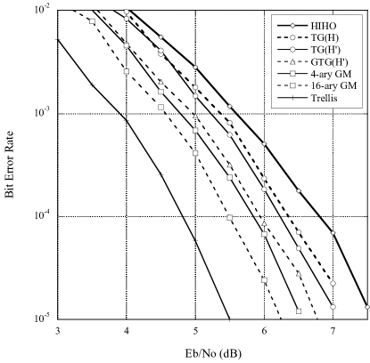
Figure 7: Bit error rate performance of different decoding algorithms for the $[64,51,6]$ extended BCH code. Fifty iterations of a flooding schedule were performed for all of the suboptimal SISO decoding algorithms.

	$N_{4}$	$N_{6}$	$N_{8}$
$\operatorname{TG}(H)$	$9827$	$1057248$	$111375740$
$\operatorname{TG}(H^{\prime})$	$3797$	$270554$	$19374579$
$\operatorname{GTG}(H^{\prime})$	$0$	$163$	$1229$
$8$-ary GM	$847$	$19590$	$304416$
$32$-ary GM	$201$	$1384$	$0$

TABLE III: Short cycle structure of the initial and extracted graphical models for the $[64,51,6]$ extended BCH code.

VII Conclusion and Future Work

This work studied the space of graphical models for a given code in order to lay out some of the foundations of the theory of extractive graphical modeling problems. The primary contributions of this work were the introduction of a new bound characterizing the tradeoff between cyclic topology and complexity in graphical models for linear codes and the introduction of a set of basic graphical model transformation operations which were shown to span the space of all graphical models for a given code. It was demonstrated that these operations can be used to extract novel cyclic graphical models - and thus novel suboptimal iterative soft-in soft-out (SISO) decoding algorithms - for linear block codes.

There are a number of interesting directions for future work motivated by the statement of the tree-inducing cut-set bound (TI-CSB). While the minimal trellis complexity $s(\mathcal{C})$ of linear codes is well-understood, less is known about minimal tree complexity $t(\mathcal{C})$ and characterizing those codes for which $t(\mathcal{C})<s(\mathcal{C})$ is an open problem. A particularly interesting open problem is the use of the Cut-Set Bound to establish an upper bound on the difference between $s(\mathcal{C})$ and $t(\mathcal{C})$; such a bound would allow for a re-expression of the TI-CSB in terms of the more familiar minimal trellis complexity. A study of those codes which meet or approach the TI-CSB is also an interesting direction for future work which may provide insight into construction techniques for good codes with short block lengths (e.g. $10$s to $100$s of bits) defined on graphs with a few cycles (e.g. $3$, $6$ or $10$). The development of statements similar to the TI-CSB for alternative measures of graphical model complexity and for graphical models of more general systems (e.g. group codes, nonlinear codes) is also interesting.

There are also a number of interesting directions for future work motivated by the study of graphical model transformation. While the extracted graphical models presented in Section VI-D are notable, ad-hoc techniques utilizing massively redundant models and judicious message filtering outperform the models presented in this work [49, 50]. Such massively redundant models contain many more short cycles than the models presented in Section VI-D indicating that short cycle structure alone is not a sufficiently meaningful cost measure for graphical model extraction. It is known that redundancy can be used to remove pseudocodewords (cf. [53]) thus motivating the study of cost measures which consider both short cycle structure and pseudocodeword spectrum. Finally, it would be interesting to study extraction heuristics beyond simple greedy searches, as well as those which use all of the basic graphical model operations (rather than just constraint merging). This appendix provides detailed definitions of both the $q^{m}$-ary graphical model properties described in Section III-B and the basic graphical model operations introduced in Section V. The proof of Lemma 1 is also further illustrated by example. In order to elucidate these properties and definitions, a single-cycle graphical model for the extended Hamming code is studied throughout.

-A Single-Cycle Model for the Extended Hamming Code

Figure 8 illustrates a single-cycle graphical model (i.e. a tail-biting trellis) for the length $8$ extended Hamming code $\mathcal{C}_{H}$.

Figure 8: Tail-biting trellis graphical model for the length $8$ extended Hamming code $\mathcal{C}_{H}$.

The hidden variables $S_{1}$ and $S_{5}$ are binary while $S_{2}$, $S_{3}$, $S_{4}$, $S_{6}$, $S_{7}$, and $S_{8}$ are $4$-ary. All of the local constraint codes in this model are interface constraints. Equations (-A)-(-A) define the local constraint codes via generator matrices (where $G_{i}$ generates $\mathcal{C}_{i}$):

$$\;\;\;\scriptstyle S_{1}\;V_{1}\;\>S_{2} \scriptstyle S_{2}\;\>V_{2}\;\;S_{3}\;\;\;\>$$

$$G_{1}= \left[\begin{array}[]{ccc}1&0&10\\ 0&1&01\end{array}\right], G_{2}=\left[\begin{array}[]{ccc}10&1&10\\ 01&1&01\end{array}\right]\>$$ (48)

$$\;\;\;\;\scriptstyle S_{3}\;\;V_{3}\;\;S_{4} \scriptstyle S_{4}\;\>V_{4}\;S_{5}\;\;\;\;\;\>$$

$$G_{3}= \left[\begin{array}[]{ccc}10&0&01\\ 01&0&11\\ 00&1&01\end{array}\right], G_{4}=\left[\begin{array}[]{ccc}10&1&0\\ 01&1&1\end{array}\right]\;\;\;$$ (54)

$$\;\;\;\scriptstyle S_{5}\;V_{5}\;\>S_{6} \scriptstyle S_{6}\;\>V_{6}\;\;S_{7}\;\;\;\>$$

$$G_{5}= \left[\begin{array}[]{ccc}1&0&10\\ 0&1&01\end{array}\right], G_{6}=\left[\begin{array}[]{ccc}10&1&10\\ 01&1&01\end{array}\right]\>$$ (59)

$$\;\;\;\;\scriptstyle S_{7}\;\;V_{7}\;\;S_{8} \scriptstyle S_{8}\;\>V_{8}\;S_{1}\;\;\;\;\;\;$$

$$G_{7}= \left[\begin{array}[]{ccc}10&0&01\\ 01&0&11\\ 00&1&01\end{array}\right], G_{8}=\left[\begin{array}[]{ccc}10&1&0\\ 01&1&1\end{array}\right].\;\;$$ (65)

The graphical model for $\mathcal{C}_{H}$ illustrated in Figure 8 is $4$-ary (i.e. $q=2$, $m=2$): the maximum hidden variable alphabet index set size is $2$ and all local constraints satisfy $\min\left(k(\mathcal{C}_{i}),n(\mathcal{C}_{i})-k(\mathcal{C}_{i})\right)\leq 2$. The behavior, $\mathfrak{B}_{H}$, of this graphical model is generated by

$$\;\;\;\>\scriptstyle S_{1}\>V_{1}\;S_{2}\;\>V_{2}\;S_{3}\;\;V_{3}\;\;S_{4}\;V_{4}\;S_{5}\;V_{5}\;S_{6}\;\;V_{6}\;\>S_{7}\;V_{7}\;\;S_{8}\;\>V_{8}$$

$$G_{\mathfrak{B}_{H}}= \left[\begin{array}[]{cccccccccccccccc}0&1&01&1&01&1&10&1&0&0&00&0&00&0&00&0\\ 0&0&00&0&00&1&01&1&1&0&10&1&10&1&00&0\\ 0&0&00&0&00&0&00&0&0&1&01&1&01&1&10&1\\ 1&0&10&1&10&1&00&0&0&0&00&0&00&1&01&1\end{array}\right].$$ (70)

The projection of $\mathfrak{B}_{H}$ onto the visible variable index set $I$, $\mathfrak{B}_{H|I}$, is thus generated by

$$\scriptstyle\;\;\;V_{1}\;\;V_{2}\;\;V_{3}\;\;V_{4}\;\;V_{5}\;\;V_{6}\;\;V_{7}\;\;V_{8}$$

$$G_{\mathfrak{B}_{H|I}}= \begin{bmatrix}1&1&1&1&0&0&0&0\\ 0&0&1&1&0&1&1&0\\ 0&0&0&0&1&1&1&1\\ 0&1&1&0&0&0&1&1\end{bmatrix}$$ (71)

which coincides precisely with a generator matrix for $\mathcal{C}_{H}$.

-B $q^{m}$-ary Graphical Model Properties

The three properties of $q^{m}$-ary graphical models introduced in Section III-B are discussed in detail in the following where it is assumed that a $q^{m}$-ary graphical model $\mathcal{G_{C}}$ with behavior $\mathfrak{B}$ for a linear code $\mathcal{C}$ over $\mathbb{F}_{q}$ defined on an index set $I$ is given.

-B1 Internal Local Constraint Involvement Property

Suppose there exists some hidden variable $S_{j}$ (involved in the local constraints $\mathcal{C}_{j_{1}}$ and $\mathcal{C}_{j_{2}}$) that does not satisfy the local constraint involvement property. A new hidden variable $S_{i}$ that is a copy of $S_{j}$ is introduced to $\mathcal{G_{C}}$ by first redefining $\mathcal{C}_{j_{2}}$ over $S_{i}$ and then inserting a local repetition constraint $\mathcal{C}_{i}$ that enforces $S_{j}=S_{i}$. The insertion of $S_{i}$ and $\mathcal{C}_{i}$ does not fundamentally alter the complexity of $\mathcal{G_{C}}$ since $n(\mathcal{C}_{i})-k(\mathcal{C}_{i})=|T_{j}|\leq m$ and since degree-$2$ repetition constraints are trivial from a decoding complexity viewpoint. Furthermore, the insertion of $S_{i}$ and $\mathcal{C}_{i}$ does not fundamentally alter the cyclic topology of $\mathcal{G_{C}}$ since no new cycles can be introduced by this procedure.

As an example, consider the binary hidden variable $S_{1}$ in Figure 8 which is incident on the interface constraints $\mathcal{C}_{1}$ and $\mathcal{C}_{8}$. By introducing the new binary hidden variable $S_{9}$ and binary repetition constraint $\mathcal{C}_{9}$, as illustrated in Figure 9, $S_{1}$ can be made to be incident on the internal constraint $\mathcal{C}_{9}$.

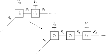
Figure 9: Insertion of hidden variable $S_{9}$ and internal local constraint $\mathcal{C}_{9}$ into the tail-biting trellis for $\mathcal{C}_{H}$.

The insertion of $S_{9}$ and $\mathcal{C}_{9}$ redefines $\mathcal{C}_{8}$ over $S_{9}$ resulting in the generator matrices

$$\;\;\;\;\scriptstyle S_{8}\;V_{8}\;S_{9} \scriptstyle S_{9}\;S_{1}\;\;\;$$

$$G_{8}= \left[\begin{array}[]{ccc}10&1&0\\ 01&1&1\end{array}\right], G_{9}=\left[\begin{array}[]{cc}1&1\end{array}\right].$$ (75)

Clearly, the modified local constraints $\mathcal{C}_{8}$ and $\mathcal{C}_{9}$ satisfy the condition for inclusion in a $4$-ary graphical model.

-B2 Internal Local Constraint Removal Property

The removal of the internal constraint $\mathcal{C}_{r}$ from $\mathcal{G_{C}}$ in order to define the new code $\mathcal{C}^{\setminus r}$ proceeds as follows. Each hidden variable $S_{i}$, $i\in I_{S}(r)$, is first disconnected from $\mathcal{C}_{r}$ and connected to a new degree-$1$ internal constraint $\mathcal{C}_{i^{\prime}}$ which does not impose any constraint on the value of $S_{i}$ (since it is degree-$1$). The local constraint $\mathcal{C}_{r}$ is then removed from the resulting graphical model yielding $\mathcal{G}_{\mathcal{C}^{\setminus r}}$ with behavior $\mathfrak{B}^{\setminus r}$. The new code $\mathcal{C}^{\setminus r}$ is the projection of $\mathfrak{B}^{\setminus r}$ onto $I$.

As an example, consider the removal of the internal local constraint $\mathcal{C}_{9}$ from the graphical model for $\mathcal{C}_{H}$ described above; the resulting graphical model update is illustrated in Figure 10. The new codes $\mathcal{C}_{10}$ and $\mathcal{C}_{11}$ are length 1, dimension 1 codes which thus impose no constraints on $S_{1}$ and $S_{9}$, respectively.

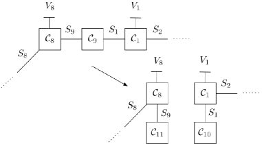
Figure 10: Removal of internal local constraint $\mathcal{C}_{9}$ from the tail-biting trellis for $\mathcal{C}_{H}$.

It is readily verified that the code $\mathcal{C}_{H}^{\setminus 9}$ which results from the removal of $\mathcal{C}_{9}$ from $\mathcal{C}_{H}$ has dimension $5$ and is generated by

$$\scriptstyle\;\;\;V_{1}\;\;V_{2}\;\;V_{3}\;\;V_{4}\;\;V_{5}\;\;V_{6}\;\;V_{7}\;\;V_{8}$$

$$G_{H^{\setminus 9}}= \begin{bmatrix}1&1&1&1&0&0&0&0\\ 0&0&1&1&0&1&1&0\\ 0&0&0&0&1&1&1&1\\ 0&1&1&0&0&0&1&1\\ 1&0&1&0&0&1&1&0\end{bmatrix}.$$ (76)

Note that $\mathcal{C}_{H}^{\setminus 9}$ corresponds to all paths in the tail-biting trellis representation of $\mathcal{C}_{H}$, not just those paths which begin and end in the same state.

The removal of an internal local constraint $\mathcal{C}_{r}$ results in the introduction of $|I_{S}(r)|$ new degree-$1$ local constraints. Forney described such constraints as “useless” in [30] and they can indeed be removed from $\mathcal{G}_{\mathcal{C}^{\setminus r}}$ since they impose no constraints on the variables they involve. Specifically, for each hidden variable $S_{i}$, $i\in I_{S}(r)$, involved in the (removed) local constraint $\mathcal{C}_{r}$, denote by $\mathcal{C}_{j}$ the other constraint involving $S_{i}$ in $\mathcal{G}_{\mathcal{C}}$. The constraint $\mathcal{C}_{j}$ can be redefined as its projection onto $I_{V}(j)\cup\left\{I_{S}(j)\setminus i\right\}$. It is readily verified that the resulting constraint $\mathcal{C}_{j}^{\setminus r}$ satisfies the condition for inclusion in a $q^{m}$-ary graphical model.

Continuing with the above example, $\mathcal{C}_{10}$, $\mathcal{C}_{11}$, $S_{1}$, and $S_{9}$ can be removed from the graphical model illustrated in Figure 10 by redefining $\mathcal{C}_{1}$ and $\mathcal{C}_{8}$ with generator matrices

$$\;\;\;\scriptstyle V_{1}\;S_{2} \scriptstyle S_{8}\;V_{8}\;\;\;\;\;\;$$

$$G_{1}= \left[\begin{array}[]{cc}1&01\\ 0&10\end{array}\right], G_{8}=\left[\begin{array}[]{cc}10&1\\ 01&1\end{array}\right].\>$$ (81)

-B3 Internal Local Constraint Redefinition Property

Let $\mathcal{C}_{i}$ satisfy $n(\mathcal{C}_{i})-k(\mathcal{C}_{i})=m^{\prime}\leq m$ and consider a hidden variable $S_{j}$ involved in $\mathcal{C}_{i}$ (i.e. $j\in I_{S}(i)$) with alphabet index set $T_{j}$. Each of the $\left|T_{j}\right|$ coordinates of $S_{j}$ can be redefined as a $q$-ary sum of some subset of the visible variable set as follows. Consider the behavior $\mathfrak{B}^{\setminus i}$ and corresponding code $\mathcal{C}^{\setminus i}$ which result when $\mathcal{C}_{i}$ is removed from $\mathcal{G_{C}}$ (before $S_{j}$ is discarded). The projection of $\mathfrak{B}^{\setminus i}$ onto $T_{j}\cup I$, $\mathfrak{B}^{\setminus i}_{|T_{j}\cup I}$, has length

$$n(\mathcal{C})+\left|T_{j}\right|$$ (82)

and dimension

$$k(\mathcal{C}^{\setminus i})\geq k(\mathcal{C})$$ (83)

over $\mathbb{F}_{q}$. There exists a generator matrix for $\mathfrak{B}^{\setminus i}_{|T_{j}\cup I}$ that is systematic in some size $k(\mathcal{C}^{\setminus i})$ subset of the index set $I$ [31]. A parity-check matrix $H_{j}$ that is systematic in the $\left|T_{j}\right|$ positions corresponding to the coordinates of $S_{j}$ can thus be found for this projection; each coordinate of $S_{j}$ is defined as a $q$-ary sum of some subset of the visible variables by $H_{j}$. Following this procedure, the internal local constraint $\mathcal{C}_{i}$ is redefined over $I$ by substituting the definitions of $S_{j}$ implied by $H_{j}$ for each $j\in I_{S}(i)$ into each of the $m^{\prime}$ $q$-ary single parity-check equations which determine $\mathcal{C}_{i}$.

Returning to the example of the tail-biting trellis for $\mathcal{C}_{H}$, the internal local constraint $\mathcal{C}_{9}$ is redefined over the visible variable set as follows. The projection of $\mathfrak{B}_{H}^{\setminus 9}$ onto $T_{1}\cup I$ is generated by

$$\scriptstyle\;\;\;S_{1}\;\;V_{1}\;\;V_{2}\;\;V_{3}\;\;V_{4}\;\;V_{5}\;\;V_{6}\;\;V_{7}\;\;V_{8}$$

$$G_{\mathfrak{B}^{\setminus 9}_{H|T_{1}\cup I}}= \begin{bmatrix}0&1&1&1&1&0&0&0&0\\ 0&0&0&1&1&0&1&1&0\\ 0&0&0&0&0&1&1&1&1\\ 1&0&1&1&0&0&0&1&1\\ 1&1&0&1&0&0&1&1&0\end{bmatrix}.$$ (84)

A valid parity-check matrix for this projection which is systematic in the position corresponding to $S_{1}$ is

$$\scriptstyle\;\;\;S_{1}\;\;V_{1}\;\;V_{2}\;\;V_{3}\;\;V_{4}\;\;V_{5}\;\;V_{6}\;\;V_{7}\;\;V_{8}$$

$$H_{1}= \begin{bmatrix}1&1&1&0&0&0&0&0&0\\ 0&1&1&1&1&0&0&0&0\\ 0&0&1&1&0&1&1&0&0\\ 0&0&1&1&0&0&0&1&1\end{bmatrix},$$ (85)

which defines the binary hidden variable $S_{1}$ as

$$S_{1}=V_{1}+V_{2}$$ (86)

where addition is over $\mathbb{F}_{2}$. A similar development defines the binary hidden variable $S_{9}$ as

$$S_{9}=V_{5}+V_{8}.$$ (87)

The local constraint $\mathcal{C}_{9}$ thus can be redefined to enforce the single parity-check equation

$$V_{1}+V_{2}+V_{5}+V_{8}=0.$$ (88)

Finally, in order to illustrate the use of the $q^{m}$-ary graphical model properties in concert, denote by $\mathcal{C}_{9}^{(1)}$ the single parity-check constraint enforcing (88). It is readily verified that only the first four rows of $G_{H^{\setminus 9}}$ (as defined in (-B2)) satisfy $\mathcal{C}_{9}^{(1)}$. It is precisely these four rows which generate $\mathcal{C}_{H}$ proving that

$$\mathcal{C}_{H}=\mathcal{C}_{H}^{\setminus 9}\cap\mathcal{C}_{9}^{(1)}.$$ (89)

-C Illustration of Proof of Lemma 1

In the following, the proof of Lemma 1 is illustrated by updating a cycle-free model for $\mathcal{C}_{H}^{\setminus 9}$ (as generated by (-B2)) with the single parity-check constraint defined by (88) in order to obtain a cycle-free graphical model for $\mathcal{C}_{H}$. A cycle-free binary graphical model for $\mathcal{C}_{H}^{\setminus 9}$ is illustrated in Figure 11.

Figure 11: Cycle-free binary graphical model for $\mathcal{C}_{H}^{\setminus 9}$. The minimal spanning tree containing the interface constraints which involve $V_{1}$, $V_{2}$, $V_{5}$, and $V_{8}$, respectively, is highlighted.

All hidden variables in Figure 11 are binary and the local constraints labeled $\mathcal{C}_{14}$, $\mathcal{C}_{17}$, $\mathcal{C}_{20}$, and $\mathcal{C}_{23}$ are binary single parity-check constraints while the remaining local constraints are repetition codes. By construction, it has thus been shown that

$$t(\mathcal{C}_{H}^{\setminus 9})=1.$$ (90)

In light of (88) and (89), a $4$-ary graphical model for $\mathcal{C}_{H}$ can be constructed by updating the graphical model illustrated in Figure 11 to enforce a single parity-check constraint on $V_{1}$, $V_{2}$, $V_{5}$, and $V_{8}$. A natural choice for the root of the minimal spanning tree containing the interface constraints incident on these variables is $\mathcal{C}_{24}$. The updating of the local constraints and hidden variables contained in this spanning tree proceeds as follows. First note that since $\mathcal{C}_{12}$, $\mathcal{C}_{15}$, $\mathcal{C}_{18}$, and $\mathcal{C}_{22}$ simply enforce equality, neither these constraints, nor the hidden variables incident on these constraints, need updating. The hidden variables $S_{14}$, $S_{17}$, $S_{20}$, and $S_{23}$ are updated to be $4$-ary so that they send downstream to $\mathcal{C}_{24}$ the values of $V_{1}$, $V_{2}$, $V_{8}$, and $V_{5}$, respectively. These hidden variable updates are accomplished by redefining the local constraints $\mathcal{C}_{14}$, $\mathcal{C}_{17}$, $\mathcal{C}_{20}$, and $\mathcal{C}_{23}$; the respective generator matrices for the redefined codes are

$$\;\;\;\scriptstyle S_{12}\;S_{13}\;S_{14} \scriptstyle S_{15}\;S_{16}\;S_{17}\;\;\;\>$$

$$G_{14}= \left[\begin{array}[]{ccc}1&0&11\\ 0&1&10\end{array}\right], G_{17}=\left[\begin{array}[]{ccc}1&0&11\\ 0&1&10\end{array}\right]\>$$ (95)

$$\;\;\;\scriptstyle S_{18}\;S_{19}\;S_{20} \scriptstyle S_{21}\;S_{22}\;S_{23}\;\;\;\>$$

$$G_{20}= \left[\begin{array}[]{ccc}1&0&11\\ 0&1&10\end{array}\right], G_{23}=\left[\begin{array}[]{ccc}1&0&10\\ 0&1&11\end{array}\right]\>$$ (100)

Finally, $\mathcal{C}_{24}$ is updated to enforce both the original repetition constraint on the respective first coordinates of $S_{14}$, $S_{17}$, $S_{20}$, and $S_{23}$ and the additional single parity-check constraint on $V_{1}$, $V_{2}$, $V_{5}$, and $V_{8}$ (which correspond to the respective second coordinates of $S_{14}$, $S_{17}$, $S_{20}$, and $S_{23}$). The generator matrix for the redefined $\mathcal{C}_{24}$ is

$$\;\;\;\;\scriptstyle S_{14}\;\;\>S_{17}\;\;\>S_{20}\;\;\>S_{23}$$

$$G_{24}= \left[\begin{array}[]{cccc}10&10&10&10\\ 01&00&00&01\\ 00&01&00&01\\ 00&00&01&01\end{array}\right].$$ (105)

The updated constraints all satisfy the condition for inclusion in a $4$-ary graphical model. Specifically, $\mathcal{C}_{24}$ can be decomposed into the Cartesian product of a length $4$ binary repetition code and a length $4$ binary single parity-check code. The updated graphical model is $4$-ary and it has thus been shown by construction that

$$t(\mathcal{C}_{H})\leq t(\mathcal{C}_{H}^{\setminus 9})+1=2.$$ (106)

-D Graphical Model Transformations

The eight basic graphical model operations introduced in Section V are discussed in detail in the following where it is assumed that a $q^{m}$-ary graphical model $\mathcal{G_{C}}$ with behavior $\mathfrak{B}$ for a linear code $\mathcal{C}$ over $\mathbb{F}_{q}$ defined on an index set $I$ is given.

-D1 Local Constraint Merging

Suppose that two local constraints $\mathcal{C}_{i_{1}}$ and $\mathcal{C}_{i_{2}}$ are to be merged. Without loss of generality, assume that there is no hidden variable incident on both $\mathcal{C}_{i_{1}}$ and $\mathcal{C}_{i_{2}}$ (since if there is, a degree-$2$ repetition constraint can be inserted). The hidden variables incident on $\mathcal{C}_{i_{1}}$ may be partitioned into two sets

$$I_{S}(i_{1})=I_{S}^{(c)}(i_{1})\cup I_{S}^{(nc)}(i_{1})$$ (107)

where each $S_{j}$, $j\in I_{S}^{(c)}(i_{1})$, is also incident on a constraint $\mathcal{C}_{j}$ which is adjacent to $\mathcal{C}_{i_{2}}$. The hidden variables incident on $\mathcal{C}_{i_{2}}$ may be similarly partitioned. The set of local constraints incident on hidden variables in both $I_{S}^{(c)}(i_{1})$ and $I_{S}^{(c)}(i_{2})$ are denoted common constraints and indexed by $I_{C}^{(c)}(i_{1},i_{2})$. Figure 12 illustrates this notation.

Figure 12: Local constraint merging notation. The local constraints $\mathcal{C}_{c_{1}}$ and $\mathcal{C}_{c_{2}}$ are common.

The merging of local constraints $\mathcal{C}_{i_{1}}$ and $\mathcal{C}_{i_{2}}$ proceeds as follows. For each common local constraint $\mathcal{C}_{j}$, $j\in I_{C}^{(c)}(i_{1},i_{2})$, denote by $S_{j_{1}}$ ($S_{j_{2}}$) the hidden variable incident on $\mathcal{C}_{j}$ and $\mathcal{C}_{i_{1}}$ ($\mathcal{C}_{i_{2}}$). Denote by $\mathcal{C}_{j|\{j_{1},j_{2}\}}$ the projection of $\mathcal{C}_{j}$ onto the two variable index set $\{j_{1},j_{2}\}$ and define a new $q^{k(\mathcal{C}_{j|\{j_{1},j_{2}\}})}$-ary hidden variable $S_{j_{1},j_{2}}$ which encapsulates the possible simultaneous values of $S_{j_{1}}$ and $S_{j_{2}}$ (as constrained by $\mathcal{C}_{j|\{j_{1},j_{2}\}}$). After defining such hidden variables for each $\mathcal{C}_{j}$, $j\in I_{C}^{(c)}(i_{1},i_{2})$, a set of new hidden variables results which is indexed by $I_{S}^{(c)}(i_{1},i_{2})$. The local constraints $\mathcal{C}_{i_{1}}$ and $\mathcal{C}_{i_{2}}$ are then merged by replacing $\mathcal{C}_{i_{1}}$ and $\mathcal{C}_{i_{2}}$ by a code defined over

$$I_{V}(i_{1})\cup I_{V}(i_{2})\cup I_{S}^{(nc)}(i_{1})\cup I_{S}^{(nc)}(i_{2})\cup I_{S}^{(c)}(i_{1},i_{2})$$ (108)

which is equivalent to $\mathcal{C}_{i_{1}}\cap\mathcal{C}_{i_{2}}$ and redefining each local constraint $\mathcal{C}_{j}$, $j\in I_{C}(i_{1},i_{2})$, over the appropriate hidden variables in $I_{S}^{(c)}(i_{1},i_{2})$.

As an example, consider again the $4$-ary cycle-free graphical model for $\mathcal{C}_{H}$ derived in the previous section, a portion of which is re-illustrated on the bottom left of Figure 13, and suppose that the local constraints $\mathcal{C}_{14}$ and $\mathcal{C}_{17}$ are to be merged. The local constraints $\mathcal{C}_{14}$, $\mathcal{C}_{17}$, and $\mathcal{C}_{24}$ are defined by (-C) and (-C).

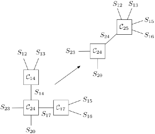
Figure 13: The merging of constraints $\mathcal{C}_{14}$ and $\mathcal{C}_{17}$ in a $4$-ary graphical model for $\mathcal{C}_{H}$. The resulting graphical model is $8$-ary.

The hidden variables incident on $\mathcal{C}_{14}$ are partitioned into the sets $I_{S}^{(c)}(14)=\{14\}$ and $I_{S}^{(nc)}(14)=\{12,13\}$. Similarly, $I_{S}^{(c)}(17)=\{17\}$ and $I_{S}^{(nc)}(17)=\{15,16\}$. The sole common constraint is thus $\mathcal{C}_{24}$. The projection of $\mathcal{C}_{24}$ onto $S_{14}$ and $S_{17}$ has dimension $3$ and the new $8$-ary hidden variable $S_{25}$ is defined by the generator matrix

$$\;\;\;\;\;\scriptstyle S_{25}\;\;\;\>S_{14}\;\;\>S_{27}$$

$$G_{14,17}= \left[\begin{array}[]{ccc}100&10&10\\ 010&01&00\\ 001&00&01\end{array}\right].$$ (112)

The local constraints $\mathcal{C}_{14}$ and $\mathcal{C}_{17}$ when defined over $S_{25}$ rather than $S_{14}$ and $S_{17}$, respectively, are generated by

$$\;\;\;\scriptstyle S_{12}\;S_{13}\;\;S_{25} \scriptstyle S_{15}\;S_{16}\;\;S_{25}\;\;\;\;\;\;\;\;$$

$$G_{14}^{\prime}= \left[\begin{array}[]{ccc}1&0&110\\ 1&0&111\\ 0&1&100\end{array}\right], G_{17}^{\prime}=\left[\begin{array}[]{ccc}1&0&101\\ 1&0&111\\ 0&1&100\end{array}\right].\>$$ (119)

Finally, $\mathcal{C}_{24}$ is redefined over $S_{25}$ and generated by

$$\;\;\;\;\;\scriptstyle S_{25}\;\;\;\>S_{20}\;\;\>S_{23}$$

$$G_{24}= \left[\begin{array}[]{ccc}100&10&10\\ 010&00&01\\ 001&00&01\\ 000&01&01\end{array}\right]$$ (124)

while $\mathcal{C}_{14}$ and $\mathcal{C}_{17}$ are replaced by $\mathcal{C}_{25}$ which is equivalent to $\mathcal{C}_{14}\cap\mathcal{C}_{17}$ and is generated by

$$\;\;\;\;\;\scriptstyle S_{25}\;\>S_{12}\>S_{13}\>S_{15}\>S_{16}\;$$

$$G_{25}= \left[\begin{array}[]{ccccc}100&0&1&0&1\\ 010&1&1&0&0\\ 001&0&0&1&1\end{array}\right].$$ (128)

Note that the graphical model which results from the merging of $\mathcal{C}_{14}$ and $\mathcal{C}_{17}$ is $8$-ary. Specifically, $S_{24}$ is an $8$-ary hidden variable while $n(\mathcal{C}_{24})-k(\mathcal{C}_{24})=3$ and $k(\mathcal{C}_{25})=3$.

-D2 Local Constraint Splitting

Local constraint splitting is simply the inverse operation of local constraint merging. Consider a local constraint $\mathcal{C}_{j}$ defined on the visible and hidden variables indexed by $I_{V}(j)$ and $I_{S}(j)$, respectively. Suppose that $\mathcal{C}_{j}$ is to be split into two local constraints $\mathcal{C}_{j_{1}}$ and $\mathcal{C}_{j_{2}}$ defined on the index sets $I_{V}(j_{1})\cup I_{S}(j_{1})$ and $I_{V}(j_{2})\cup I_{S}(j_{2})$, respectively, such that $I_{V}(j_{1})$ and $I_{V}(j_{2})$ partition $I_{V}(j)$ while $I_{S}(j_{1})\cup I_{S}(j_{2})=I_{S}(j)$ but $I_{S}(j_{1})$ and $I_{S}(j_{2})$ need not be disjoint. Denote by $I_{S}(j_{1},j_{2})$ the intersection of $I_{S}(j_{1})$ and $I_{S}(j_{2})$. Local constraint splitting proceeds as follows. For each $S_{i}$, $i\in I_{S}(j_{1},j_{2})$, make a copy $S_{i^{\prime}}$ of $S_{i}$ and redefine the local constraint incident on $S_{i}$ (which is not $\mathcal{C}_{j}$) over both $S_{i}$ and $S_{i^{\prime}}$. Denote by $I_{S}^{\prime}(j_{1},j_{2})$ an index set for the copied hidden variables. The local constraint $\mathcal{C}_{j}$ is then replaced by $\mathcal{C}_{j_{1}}$ and $\mathcal{C}_{j_{2}}$ such that $\mathcal{C}_{j_{1}}$ is defined over $I_{V}(j_{1})\cup I_{S}(j_{1})$ and $\mathcal{C}_{j_{2}}$ is defined over

$$I_{V}(j_{2})\cup I_{S}(j_{2})\setminus I_{S}(j_{1},j_{2})\cup I_{S}^{\prime}(j_{1},j_{2}).$$ (129)

Following this split procedure, some of the hidden variables in $I_{S}(j_{1},j_{2})$ and $I_{S}^{\prime}(j_{1},j_{2})$ may have larger alphabets than necessary. Specifically, if the dimension of the projection of $\mathcal{C}_{j_{1}}$ ($\mathcal{C}_{j_{2}}$) onto a variable $S_{i}$, $i\in I_{S}(j_{1},j_{2})$ ($i\in I_{S}^{\prime}(j_{1},j_{2})$), is smaller than the alphabet index set size of $S_{i}$, then $S_{i}$ can be redefined with an alphabet index set size equal to that dimension.

The merged code in the example of the previous section $\mathcal{C}_{25}$ can be split into two codes: $\mathcal{C}_{14}$ defined on $S_{12}$, $S_{13}$, and $S_{24}$, and $\mathcal{C}_{17}$ defined on $S_{15}$, $S_{16}$, and $S_{24^{\prime}}$. The projection of $S_{24}$ onto $\mathcal{C}_{14}$ has dimension $2$ and $S_{24}$ can thus be replaced by the $4$-ary hidden variable $S_{14}$. Similarly, the projection of $S_{24^{\prime}}$ onto $\mathcal{C}_{17}$ has dimension $2$ and $S_{24^{\prime}}$ can be replaced by the $4$-ary hidden variable $S_{17}$.

-D3 Insertion/Removal of Degree-$2$ Repetition Constraints

Suppose that $S_{i}$ is a hidden variable involved in the local constraints $\mathcal{C}_{i_{1}}$ and $\mathcal{C}_{i_{2}}$. A degree-$2$ repetition constraint is inserted by defining a new hidden variable $S_{j}$ as a copy of $S_{i}$, redefining $\mathcal{C}_{i_{2}}$ over $S_{j}$ and defining the repetition constraint $\mathcal{C}_{j}$ which enforces $S_{i}=S_{j}$. Degree-$2$ repetition constraint insertion can be similarly defined for visible variables. Conversely, suppose that $\mathcal{C}_{j}$ is a degree-$2$ repetition constraint incident on the hidden variables $S_{i}$ and $S_{j}$. Since $\mathcal{C}_{j}$ simply enforces $S_{i}=S_{j}$, it can be removed and $S_{j}$ relabeled $S_{i}$. Degree-$2$ repetition constraint removal can be similarly defined for visible variables. The insertion and removal of degree-$2$ repetition constraints is illustrated in Figures 14 and 14 for hidden and visible variables, respectively.

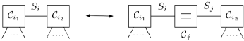
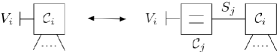
Figure 14: Insertion and removal of degree-$2$ repetition constraints.

-D4 Insertion/Removal of Trivial Constraints

Trivial constraints are those incident on no hidden or visible variables so that their respective block lengths and dimensions are zero. Trivial constraints can obviously be inserted or removed from graphical models.

-D5 Insertion/Removal of Isolated Partial Parity-Check Constraints

Suppose that $\mathcal{C}_{i_{1}},\ldots,\mathcal{C}_{i_{j}}$ are $j$ $q$-ary repetition constraints (that is each repetition constraint enforces equality on $q$-ary variables) and let $\beta_{i_{1}},\ldots,\beta_{i_{j}}\in\mathbb{F}_{q}$ be non-zero. The insertion of an isolated partial parity-check constraint is defined as follows. Define $j+1$ new $q$-ary hidden variables $S_{i_{1}},\ldots,S_{i_{j}}$ and $S_{k}$, and two new local constraints $\mathcal{C}_{p}$ and $\mathcal{C}_{k}$ such that $\mathcal{C}_{p}$ enforces the $q$-ary single parity-check equation

$$\sum_{l=1}^{j}\beta_{i_{l}}S_{i_{l}}=S_{k}$$ (130)

and $\mathcal{C}_{k}$ is a degree-$1$ constraint incident only on $S_{k}$ with dimension $1$. The new local constraint $\mathcal{C}_{p}$ defines the partial parity variable $S_{k}$ and is denoted isolated since it is incident on a hidden variable which is involved in a degree-$1$, dimension $1$ local constraint (i.e. $\mathcal{C}_{k}$ does not constrain the value of $S_{k}$). Since $\mathcal{C}_{p}$ is isolated, the graphical model that results from its insertion is indeed a valid model for $\mathcal{C}$. Similarly, any such isolated partial parity-check constraint can be removed from a graphical model resulting in a valid model for $\mathcal{C}$.

As an example, Figure 15 illustrates the insertion and removal of an isolated partial-parity check on the binary sum of $V_{7}$ and $V_{8}$ in a Tanner graph for $\mathcal{C}_{H}$ corresponding to (-A) (note that $\mathcal{C}_{H}$ is self-dual so that the generator matrix defined in (-A) is also a valid parity-check matrix for $\mathcal{C}_{H}$).

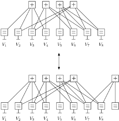
Figure 15: The insertion/removal of an isolated partial parity-check constraint on $V_{7}$ and $V_{8}$ in a Tanner graph for $\mathcal{C}_{H}$.

References

- [1] C. Berrou, A. Glavieux, and P. Thitmajshima, “Near Shannon limit error-correcting coding and decoding: Turbo-codes,” in Proc. International Conf. Communications, Geneva, Switzerland, May 1993, pp. 1064–1070.
- [2] R. G. Gallager, “Low density parity check codes,” IEEE Trans. Information Theory, vol. 8, pp. 21–28, January 1962.
- [3] M. Sipser and D. A. Spielman, “Expander codes,” IEEE Trans. Information Theory, vol. 42, pp. 1660–1686, November 1996.
- [4] D. J. C. MacKay, “Good error-correcting codes based on very sparse matrices,” IEE Electronics Letters, vol. 33, pp. 457–458, March 1997.
- [5] N. Wiberg, H.-A. Loeliger, and R. Kötter, “Codes and iterative decoding on general graphs,” European Trans. Telecommun., vol. 6, no. 5, pp. 513–525, Sept-Oct. 1995.
- [6] N. Wiberg, “Codes and decoding on general graphs,” Ph.D. dissertation, Linköping University (Sweden), 1996.
- [7] S. M. Aji and R. J. McEliece, “The generalized distributive law,” IEEE Trans. Information Theory, vol. 46, no. 2, pp. 325–343, March 2000.
- [8] K. M. Chugg, A. Anastasopoulos, and X. Chen, Iterative Detection: Adaptivity, Complexity Reduction, and Applications. Kluwer Academic Publishers, 2001.
- [9] F. Kschischang, B. Frey, and H.-A. Loeliger, “Factor graphs and the sum-product algorithm,” IEEE Trans. Information Theory, vol. 47, pp. 498–519, Feb. 2001.
- [10] G. D. Forney, Jr., “Codes on graphs: Normal realizations,” IEEE Trans. Information Theory, pp. 520–548, February 2001.
- [11] R. M. Tanner, “A recursive approach to low complexity codes,” IEEE Trans. Information Theory, vol. IT-27, pp. 533–547, September 1981.
- [12] Y. Mao and A. H. Banihashemi, “A heuristic search for good low-density parity-check codes at short block lengths,” in Proc. International Conf. Communications, vol. 1, Helsinki, Finland, June 2001, pp. 41–44.
- [13] D. M. Arnold, E. Eleftheriou, and X. Y. Hu, “Progressive edge-growth Tanner graphs,” in Proc. Globecom Conf., vol. 2, San Antonion, TX, November 2001, pp. 995–1001.
- [14] X.-P. Ge, D. Eppstein, and P. Smyth, “The distribution of loop lengths in graphical models for turbo decoding,” IEEE Trans. Information Theory, vol. 47, no. 6, pp. 2549–2553, September 2001.
- [15] T. Tian, C. R. Jones, J. D. Villasenor, and R. D. Wesel, “Selective avoidance of cycles in irregular LDPC code construction,” IEEE Trans. Information Theory, vol. 52, no. 8, pp. 1242–1247, August 2004.
- [16] T. R. Halford and K. M. Chugg, “An algorithm for counting short cycles in bipartite graphs,” IEEE Trans. Information Theory, vol. 52, no. 1, pp. 287–292, January 2006.
- [17] S. Y. Chung, G. D. Forney, Jr., T. J. Richardson, and R. Urbanke, “On the design of low-density parity-check codes within 0.0045 dB of the Shannon limit,” IEEE Communications Letters, vol. 5, no. 2, pp. 58–60, February 2001.
- [18] T. Richardson, M. Shokrollahi, and R. Urbanke, “Design of capacity-approaching irregular low-density parity-check codes,” IEEE Trans. Information Theory, vol. 47, no. 2, pp. 619–673, February 2001.
- [19] P. Oswald and A. Shokrollahi, “Capacity-achieving sequences for the erasure channel,” IEEE Trans. Information Theory, vol. 48, no. 12, pp. 3017–3028, December 2002.
- [20] H. D. Pfister, I. Sason, and R. Urbanke, “Capacity-achieving ensembles for the binary erasure channel with bounded complexity,” IEEE Trans. Information Theory, vol. 51, no. 7, pp. 2352–2379, July 2005.
- [21] S. Benedetto and G. Montorsi, “Design of parallel concatenated convolutional codes,” IEEE Trans. Communications, vol. 44, pp. 591–600, May 1996.
- [22] S. Dolinar, D. Divsalar, and F. Pollara, “Code performance as a function of block size,” Jet Propulsion Labs., Pasadena, CA, Tech. Rep. TDA Progress Report 42-133, May 1998.
- [23] C. Berrou, “The ten-year-old turbo codes are entering into service,” IEEE Communications Mag., vol. 41, no. 8, pp. 110–116, August 2003.
- [24] S. ten Brink, “Convergence behavior of iteratively decoded parallel concatenated codes,” IEEE Trans. Communications, vol. 49, no. 10, pp. 1727–1737, October 2001.
- [25] K. M. Chugg, P. Thiennviboon, G. D. Dimou, P. Gray, and J. Melzer, “A new class of turbo-like codes with universally good performance and high-speed decoding,” in Proc. IEEE Military Comm. Conf., Atlantic City, NJ, October 2005.
- [26] T. R. Halford, A. J. Grant, and K. M. Chugg, “Which codes have 4-cycle-free Tanner graphs?” IEEE Trans. Information Theory, vol. 52, no. 9, pp. 4219–4223, September 2006.
- [27] A. Vardy, Handbook of Coding Theory. Amsterdam, The Netherlands: Elsevier, 1999, ch. Trellis structure of codes, eds.: V. S. Pless and W. C. Huffman.
- [28] A. R. Calderbank, G. D. Forney, Jr., and A. Vardy, “Minimal tail-biting trellises: The Golay code and more,” IEEE Trans. Information Theory, vol. 45, no. 5, pp. 1435–1455, July 1999.
- [29] R. Koetter and A. Vardy, “The structure of tail-biting trellises: Minimality and basic principles,” IEEE Trans. Information Theory, vol. 49, pp. 2081–2105, September 2003.
- [30] G. D. Forney, Jr., “Codes on graphs: Constraint complexity of cycle-free realizations of linear codes,” IEEE Trans. Information Theory, vol. 49, no. 7, pp. 1597–1610, July 2003.
- [31] F. J. MacWilliams and N. J. A. Sloane, The Theory of Error-Correcting Codes. North-Holland, 1978.
- [32] D. J. C. MacKay, “Relationships between sparse graph codes,” in Proc. Information-Based Induction Sciences, Izu, Japan, July 2000.
- [33] J. S. Yedidia, J. Chen, and M. C. Fossorier, “Generating code representations suitable for belief propagation decoding,” in Proc. Allerton Conf. Commun., Control, Comp., Monticello, IL, October 2002.
- [34] A. Lafourcade and A. Vardy, “Lower bounds on trellis complexity of block codes,” IEEE Trans. Information Theory, vol. 41, no. 6, pp. 1938–1954, November 1995.
- [35] D. J. Muder, “Minimal trellises for block codes,” IEEE Trans. Information Theory, vol. 34, no. 5, pp. 1049–1053, September 1988.
- [36] Y. Berger and Y. Be’ery, “Bounds on the trellis size of linear block codes,” IEEE Trans. Information Theory, vol. 39, no. 1, pp. 203–209, January 1993.
- [37] T. Kasami, T. Takata, T. Fujiwara, and S. Lin, “On the optimum bit orders with respect to the state complexity of trellis diagrams for binary linear codes,” IEEE Trans. Information Theory, vol. 39, no. 1, pp. 242–245, January 1993.
- [38] ——, “On complexity of trellis structure of linear block codes,” IEEE Trans. Information Theory, vol. 39, no. 3, pp. 1057–1064, May 1993.
- [39] G. D. Forney, Jr., “Density/length profiles and trellis complexity of linear block codes,” IEEE Trans. Information Theory, vol. 40, no. 6, pp. 1741–1752, November 1994.
- [40] T. R. Halford and K. M. Chugg, “Conditionally cycle-free generalized Tanner graphs: Theory and application to high-rate serially concatenated codes,” Communication Sciences Institute, USC, Los Angeles, CA, Tech. Rep. CSI-06-09-01, September 2006.
- [41] R. Diestel, Graph Theory, 2nd ed. New York, NY: Springer-Verlag, 2000.
- [42] Y. Wang, R. Ramesh, A. Hassan, and H. Koorapaty, “On MAP decoding for tail-biting convolutional codes,” in Proc. IEEE International Symp. on Information Theory, Ulm, Germany, June 1997, p. 225.
- [43] S. M. Aji, G. B. Horn, and R. J. McEliece, “Iterative decoding on graphs with a single cycle,” in Proc. IEEE International Symp. on Information Theory, Cambridge, MA, August 1998, p. 276.
- [44] J. B. Anderson and S. M. Hladik, “Tailbiting MAP decoders,” IEEE J. Select. Areas Commun., vol. 16, no. 2, pp. 297–302, February 1998.
- [45] J. Heo and K. M. Chugg, “Constrained iterative decoding: Performance and convergence analysis,” in Proc. Asilomar Conf. Signals, Systems, Comp., Pacific Grove, CA, November 2001, pp. 275–279.
- [46] Y. Shany and Y. Be’ery, “Linear tail-biting trellises, the square-root bound, and applications for Reed-Muller codes,” IEEE Trans. Information Theory, vol. 46, no. 4, pp. 1514–1523, July 2000.
- [47] J. K. Wolf, “Efficient maximum-likelihood decoding of linear block codes using a trellis,” IEEE Trans. Information Theory, vol. 24, pp. 76–80, 1978.
- [48] R. J. McEliece, “On the BCJR trellis for linear block codes,” IEEE Trans. Information Theory, vol. 42, no. 4, pp. 1072–1092, July 1996.
- [49] J. Jiang and K. R. Narayanan, “Iterative soft decision decoding of Reed-Solomon codes,” IEEE Communications Letters, vol. 8, no. 4, pp. 244–246, April 2004.
- [50] T. R. Halford and K. M. Chugg, “Random redundant soft-in soft-out decoding of linear block codes,” presented at ISIT 2006.
- [51] S. Sankaranarayanan and B. Vasić, “Iterative decoding of linear block codes: A parity-check orthogonalization approach,” IEEE Trans. Information Theory, vol. 51, no. 9, pp. 3347–3353, September 2005.
- [52] V. Kumar and O. Milenkovic, “On graphical representations for algebraic codes suitable for iterative decoding,” IEEE Communications Letters, vol. 9, no. 8, pp. 729–731, August 2005.
- [53] P. O. Vontobel and R. Koetter, “Graph-cover decoding and finite-length analysis of message-passing iterative decoding of LDPC codes,” December 2005, submitted to IEEE Trans. Information Theory.