T-Theory Applications to Online Algorithms
for the Server Problem

Abstract

Although largely unnoticed by the online algorithms community, T-theory, a field of discrete mathematics, has contributed to the development of several online algorithms for the $k$-server problem. A brief summary of the $k$-server problem, and some important application concepts of T-theory, are given. Additionally, a number of known $k$-server results are restated using the established terminology of T-theory. Lastly, a previously unpublished 3-competitiveness proof, using T-theory, for the Harmonic algorithm for two servers is presented.

Keywords/Phrases: Double Coverage, Equipoise, Harmonic, Injective Hull, Isolation Index, Prime Metric, Random Slack, T-Theory, Tight Span, Trackless Online Algorithm

1 Introduction

The $k$-server problem was introduced by Manasse, McGeoch, and Sleator [65], while T-theory was introduced by John Isbell [57] and independently rediscovered by Andreas Dress [39, 40]. The communities of researchers in these two areas have had little interaction. The tight span, a fundamental construction of T-theory, was later defined independently, using different notation, by Chrobak and Larmore, who were unaware of the work of Isbell, Dress, and others.

Bartal [6], Chrobak and Larmore [26, 28, 29, 32], and Teia [72], have used the tight span concept to obtain results for the $k$-server problem. In this paper, we summarize those results, using the standard notation of T-theory. We then suggest ways to use T-theory to obtain additional results for the $k$-server problem.

1.1 The $k$-Server Problem

Let $M$ be a metric space, in which there are $k$ identical mobile servers. At each time step a request point $r\in M$ is given, and one server must move to $r$ to serve the request. The measure of cost is the total distance traveled by the servers over the entire sequence of requests.

An online algorithm is an algorithm which must decide on some outputs before knowing all inputs. Specifically, an online algorithm for the server problem must decide which server to move to a given request point, without knowing the sequence of future requests, as opposed to an offline algorithm, which knows all requests in advance.

For any constant $C\geq 1$ we say that an online algorithm ${\cal A}$ for the server problem is $C$-competitive if there exists a constant $K$ such that, for any request sequence $\varrho$, where ${\mbox{\it cost\/}}_{{}_{{\mbox{\scriptsize\sc opt}}}}(\varrho)$ is the optimum cost for serving that sequence:

$${\mbox{\it cost\/}}_{{}_{{\cal A}}}(\varrho)\leq C\cdot{\mbox{\it cost\/}}_{{}_{{\mbox{\scriptsize\sc opt}}}}(\varrho)+K$$

If ${\cal A}$ is randomized, the expected cost $E{\mbox{\it cost\/}}_{{}_{{\cal A}}}(\varrho)$ is used instead of ${\mbox{\it cost\/}}_{{}_{{\cal A}}}(\varrho)$.

The $k$-server conjecture, posed by Manasse, McGeoch, and Sleator [65], is that there is a deterministic $k$-competitive online algorithm for the $k$-server problem in an arbitrary metric space. Since its introduction by Manasse et al., substantial work has been done on the $k$-server problem [1, 2, 6, 7, 8, 9, 10, 12, 13, 11, 15, 16, 18, 19, 20, 21, 31, 33, 34, 36, 46, 47, 48, 49, 50, 51, 56, 58, 64, 62, 72, 73]. The $k$-server conjecture remains open, except for special cases, and for $k=2$ for all cases.

It is traditional to analyze the competitiveness of an online algorithm by imagining the existence of an adversary, who creates the request sequence, and must also serve that same sequence. Since we assume that the adversary has unlimited computational power, it will serve the request sequence optimally; thus, competitiveness can be calculated by comparing the cost incurred by the online algorithm to the cost incurred by that adversary. We refer the reader to Chapter 4 of [21] for an extensive discussion of adversarial models.

Throughout this paper, we will let $s_{{}_{1}},\ldots,s_{{}_{k}}$ denote the algorithm’s servers, and also, by an abuse of notation, the points where the servers are located. Similarly, we will let $a_{{}_{1}},\ldots,a_{{}_{k}}$ denote both the adversary’s servers and the points where they are located. We will also let $r$ be the request point.

1.2 Memoryless, Fast, and Trackless $k$-Server Algorithms

Let ${\cal A}$ be an online algorithm for the $k$-server problem. ${\cal A}$ is called memoryless if its only memory between steps is the locations of its own servers. When a new request is received, ${\cal A}$ makes a decision, moves its servers, and then forgets all information except the new locations of the servers.

${\cal A}$ is called fast if, after each request, ${\cal A}$ can make its decision using $O(1)$ operations, where computing the distance between two points counts as one operation.

${\cal A}$ is called trackless if ${\cal A}$ initially knows only the distances between its various servers. When ${\cal A}$ receives a request, it is only told the distances between that request and each of its servers. ${\cal A}$’s only allowed output is an instruction to move a specific server to the request point. ${\cal A}$ may not have any naming system for points. Thus, it cannot tell how close a given request is to any point on which it does not currently have a server. See [17] for further discussion of tracklessness.

1.3 The Lazy Adversary

The lazy adversary is an adversary that always makes a request that costs it nothing to serve, but which forces the algorithm to pay, if such a request is possible. For the $k$-server problem, the lazy adversary always requests a point where one of its servers is located, provided the algorithm has no server at that point. When all algorithm servers are at the same points as the adversary servers, the lazy adversary may move one of its servers to a new point. Thus, the lazy adversary never has more than one server that is in a position different from that of an algorithm server. Some online algorithms, such as handicap, introduced in Section 7, perform better against the lazy adversary than against an adversary without that restriction.

1.4 T-Theory and its Application to the $k$-Server Problem

Since the pioneering work by Isbell and Dress, there have been many contributions to the field of T-theory [3, 4, 5, 22, 23, 24, 41, 38, 42, 43, 44, 45, 52, 53, 54, 55, 57, 59, 60, 69, 70]. The original motivation for the development of T-theory, and one of its most important application areas, is phylogenetic analysis, the problem of constructing a phylogenetic tree showing relationships among species or languages [14, 68].

It was first discovered by Chrobak and Larmore [26] that T-theory can aid in the competitive analysis of online algorithms for the $k$-server problem. Since then, work by Teia [72] and Bartal [6], and additional work by Chrobak and Larmore [28, 32] have made use of T-theory concepts to obtain $k$-server results.

Many proofs of results in the area of the $k$-server problem require lengthy case-by-case analysis. T-theory can help guide this process by providing a natural way to break a proof or a definition into cases. This can be seen in this paper in the definitions of balance slack §5.2 and handicap §5.3, and in the proof of 3-competitiveness of harmonic for $k=2$, in Section 8.

In a somewhat different use of T-theory, the tight span algorithm and equipoise make use of the virtual server method discussed in Section 3. These algorithms move servers virtually in the tight span of a metric space.

1.5 Overview of the Paper

In Section 2, we give some elementary constructions from T-theory that are used in applications to the server problem. We provide illustrations and pseudo code for a number of algorithms that we describe.

In Section 3, we give the virtual server construction, which is used for the tight span algorithm as well as for equipoise. In §4.2, we describe the tree algorithm (tree) of [29], which forms the basis of a number of the other server algorithms described in this paper. In §4.3, we describe the Bartal’s Slack Coverage algorithm for 2 servers in a Euclidean space [6] in terms of T-theory.

In Section 5, we discuss balance algorithms for the $k$-server problem in terms of $T$-theory. In Section 6 we describe the tight span algorithm [26] and equipoise [32] in terms of T-theory. In Section 7, we present a description of Teia’s algorithm handicap. In §8.2 we describe how the algorithm random slack is defined using T-theory. In §8.3, we present a T-theory based proof that harmonic [66] is 3-competitive for $k=2$. In Section 9, we discuss possible future uses of T-theory for the $k$-server problem.

We present a simplified proof that handicap is $k$-competitive against certain adversaries (Theorem 3), based on the proof in Teia’s disseration [72]. We also give a previously unpublished proof that harmonic is 3-competitive for $k=2$.

2 Elementary T-Theory Concepts

In keeping with the usual practice of T-theory papers, we extend the meaning of the term metric to incorporate what is commonly called a pseudo-metric. That is, we define a metric on a set $X$ to be a function $d:X\times X\to{\bf R}$ such that

1. $d(x,x)=0$ for all $x\in X$

2. $d(x,y)=d(y,x)$ for all $x,y\in X$

3. $d(x,y)+d(y,z)\geq d(x,z)$ for all $x,y,z\in X$ (Triangle Inequality)

We say that $d$ is a proper metric if, in addition, $d(x,y)>0$ whenever $x\neq y$. We also adopt the usual practice of abbreviating a metric space $(X,d)$ as simply $X$, if $d$ is understood.

2.1 Injective Spaces and the Tight Span

Isbell [57] defines a metric space $M$ to be injective if, for any metric space $Y\supseteq M$, there is a non-expansive retraction of $Y$ onto $M$, i.e., a map $r:Y\to M$ which is the identity on $M$, where $d(r(x),r(y))\leq d(x,y)$ for all $x,y\in Y$. The real line, the Manhattan plane, i.e., the plane ${\bf R}^{2}$ with the ${\cal L}_{1}$ (sum of norms) metric, and ${\bf R}^{n}$ with the ${\cal L}_{\infty}$ (sup-norm) metric, where the distance between ${\left(x_{{}_{1}},\ldots,x_{{}_{n}}\right)}$ and ${\left(y_{{}_{1}},\ldots,y_{{}_{n}}\right)}$ is $\max_{1\leq i\leq n}{\left|x_{{}_{i}}-y_{{}_{i}}\right|}$, are injective. No Euclidean space of dimension more than one is injective.

Figure 1: Illustration of $L_{1}$, $L_{2}$, and $L_{\infty}$ metrics on the plane. The distance between $x$ and $y$ is 9 with the $L_{1}$ metric, $\sqrt{41}$ with the $L_{2}$ metric and 5 with the $L_{\infty}$ metric.

The tight span $T(X)$ of a metric space $X$, which we formally define below, is characterized by a universal property: up to isomorphism, $T(X)$ is the unique minimal injective metric space that contains $X$. Thus, $X=T(X)$ if and only if $X$ is injective.

Isbell [57] was the first to construct $T(X)$, which he called the injective hull of $X$. Dress [39] independently developed the same construction, naming it the tight span of $X$. Still later, Chrobak and Larmore also independently developed the tight span, which they called the abstract convex hull of $X$.

We now give a formal construction of $T(X)$. Let

$$P(X)={\left\{f\in{\bf R}^{X}\ |\ f(x)+f(y)\geq d(x,y){\ {\mbox{\rm for all}}\ }x,y\in X\right\}}$$ (1)

where ${\bf R}^{X}$ is the set of all functions $f:X\to{\bf R}$, and let $T(X)\subseteq P(X)$ be the set of those functions which are minimal with respect to pointwise partial order. $T(X)$ is a metric space where distance is given by the sup-norm metric, i.e., If $f,g\in T(X)$, we define $d(f,g)=\sup_{x\in X}{\left|f(x)-g(x)\right|}$. If $X$ is finite, then $P(X)$ is also a metric space under the sup-norm metric, and is called the associated polytope of $X$ [59]. There is a canonical embedding of $X$ into $T(X)$. For any $x\in X$, let $h_{{}_{x}}\in T(X)$ be the function where $h_{{}_{x}}(y)=d(x,y)$ for all $y$. By an abuse of notation, we identify each $x$ with $h_{{}_{x}}$, and thus say $X\subseteq T(X)$.

If $X$ has cardinality $n$, then $P(X)\subseteq{\bf R}^{X}\cong{\bf R}^{n}$. For any $x,y\in X$, let $D_{x,y}\subseteq{\bf R}^{X}$ be the half-space defined by the inequality $f(x)+f(y)\geq d(x,y)$, and let $H_{x,y}\subseteq{\bf R}^{X}$ be the boundary of $D_{x,y}$, the hyperplane defined by the equation $f(x)+f(y)=d(x,y)$, which we call a bounding hyperplane of $P(X)$. Then $P(X)=\bigcap_{x,y\in X}D_{x,y}$ is an unbounded convex polytope of dimension $n$, and $T(X)$ is the union of all the bounded faces of $P(X)$.

The definition of convex subset of a metric space is not consistent with the definition of convex subset of a vector space over the real numbers. $T(X)$ is a convex subset of $P(X)$, if $P(X)$ is considered to be a metric space; but $T(X)$ is not generally a convex subset of ${\bf R}^{X}$ if ${\bf R}^{X}$ is considered to be a vector space over ${\bf R}$.

Figure 2: A two-dimensional projection of the three-dimensional complex $P(X)$, in the case where $X$ is the 3-4-5 triangle. $T(X)$ is the subcomplex consisting of the vertices and the bold line segments.

Figure 3: A view of the tight span of the 3-4-5 triangle, embedded in $({\bf R}^{3},{\cal L}_{\infty})$.

Figure 4: A view of the associated polytope of the 3-4-5 triangle, with the tight span in bold.

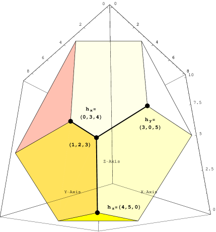
Dress proves [40] that the tight span of a metric space of cardinality $n$ is a cell complex, where each cell is a polytope of dimension at most ${\left\lfloor\frac{n}{2}\right\rfloor}$. In Figures 2, 4, and 4, we give an example of the tight span of the 3-4-5 triangle. Let $X={\left\{x,y,z\right\}}$, where $d(x,y)=3$, $d(x,z)=4$, and $d(y,z)=5$. The vertices of $T(X)$, represented as 3-tuples in ${\bf R}^{3}\cong{\bf R}^{X}$, are

$$h_{x}=(0,3,4) = H_{x,x}\cap H_{x,y}\cap H_{x,z}$$

$$h_{y}=(3,0,5) = H_{x,y}\cap H_{y,y}\cap H_{y,z}$$

$$h_{z}=(4,5,0) = H_{x,z}\cap H_{y,z}\cap H_{z,z}$$

$$(1,2,3) = H_{x,y}\cap H_{x,z}\cap H_{y,z}$$

Figure 2 shows a projection of $P(X)$ in two dimensions. The boundary of $P(X)$ consists of four vertices, three bounded edges, six unbounded edges, and six unbounded 2-faces. $T(X)$ is the union of the bounded edges. Figure 4 is a perspective showing $T(X)$ in ${\bf R}^{3}$, which we endow with the ${\cal L}_{\infty}$ metric. Figure 4 is a rendering of the polytope obtained by intersecting $P(X)$ with a half space.

2.2 The Isolation Index and the Split Decomposition

Let $(X,d)$ be a metric space. If $A,B\subseteq X$ are non-empty subsets of $X$, Bandelt and Dress [5] (page 54) define the isolation index of the pair ${\left\{A,B\right\}}$ to be

$$\alpha_{{}_{A,B}}={\mbox{$\frac{1}{2}$}}\min_{a,a^{\prime}\in A\atop b,b^{\prime}\in B}{\left\{\max{\left\{0,d(a,b)+d(a^{\prime},b^{\prime})-d(a,a^{\prime})-d(b,b^{\prime}),d(a,b^{\prime})+d(a^{\prime},b)-d(a,a^{\prime})-d(b,b^{\prime})\right\}}\right\}}\rule{21.68121pt}{0.0pt}$$

Observation 1

$\alpha_{{}_{{\left\{x\right\}},{\left\{y,z\right\}}}}=\frac{d(x,y)+d(x,z)-d(y,z)}{2}$ for any three points $x,y,z$.

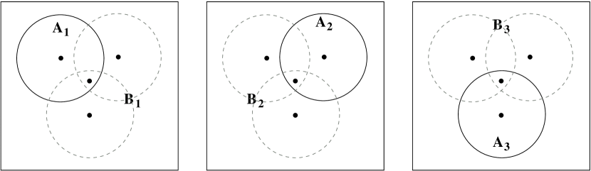
A split of a metric space $(X,d)$ is a partition of the points of $X$ into two non-empty sets. We say that a split $A,B$ separates two points if one of the points is in $A$ and the other in $B$. We will use Fraktur letters for sets of splits. If $\mathfrak{S}$ is a set of splits of $X$, we say that $\mathfrak{S}$ is weakly compatible if, given any four point set $Y\subseteq X$ and given any three members of $\mathfrak{S}$, namely ${\left\{A_{1},B_{1}\right\}}$, ${\left\{A_{2},B_{2}\right\}}$, and ${\left\{A_{3},B_{3}\right\}}$, the sets $A_{1}\cap Y$, $B_{1}\cap Y$, $A_{2}\cap Y$, $B_{2}\cap Y$, $A_{3}\cap Y$, and $B_{3}\cap Y$ do not consist of all six two point subsets of $Y$. Figure 5 shows an example of three splits which are not weakly compatible.

Figure 5: Three splits which are not weakly compatible

If $\alpha_{{}_{S}}>0$, we say that $S$ is a $d$-split of $X$. The set of all $d$-splits of $X$ is always weakly compatible. For more information regarding weak compatibility, see [24]. From Bandelt and Dress [5], we say that $(X,d)$ is split-prime if $X$ has no $d$-splits. For any split $S$ the split metric on $X$ is defined as

$$\delta_{{}_{S}}(x,y)=\left\{\begin{array}[]{l}1{\ {\mbox{\rm if}}\ }S{\ {\mbox{\rm separates}}\ }{\left\{x,y\right\}}\\ 0{\ {\mbox{\rm otherwise}}}\end{array}\right.$$

The split decomposition of $(X,d)$ is defined to be

$$d=d_{{}_{0}}+\sum_{S\in\mathfrak{S}}\alpha_{{}_{S}}\delta_{{}_{S}}$$

where $\mathfrak{S}$ is the set of all $d$-splits of $X$, and $d_{{}_{0}}$ is called the split-prime residue of $d$. The split decomposition of $d$ is unique. If $d_{{}_{0}}=0$, we say that $d$ is totally decomposable. From Bandelt and Dress [5], we have

Lemma 1

Every metric on four or fewer points is totally decomposable.

Observation 2

If $X$ is totally decomposable and $x,y\in X$, then

$$d(x,y)=\sum_{S{\ {\mbox{\rm\tiny separates}}\ }\atop{\left\{x,y\right\}}}\alpha_{{}_{S}}\delta_{{}_{S}}$$

More generally:

Observation 3

If $d_{{}_{0}}$ is the split-prime residue of $X$, and if $x,y\in X$, then

$$d(x,y)=d_{{}_{0}}(x,y)+\sum_{S{\ {\mbox{\rm\tiny separates}}\ }\atop{\left\{x,y\right\}}}\alpha_{{}_{S}}\delta_{{}_{S}}$$

In Figure 6, we show how the computations of all $d$-splits for the 3-4-5 triangle and the resulting tight span of that space.

2.3 T-Theory and Trees

The original inspiration for the study of T-theory was the problem of measuring how “close” a given metric space is to being embeddable into a tree. This question is important in phylogenetic analysis, the analysis of relations among species or languages [14, 68], since we would like to map any set of species or languages onto a phylogenetic tree which represents their actual descent, using a metric which represents the difference between any two members of the set. We say that a metric space $M$ is a tree if, given any two points $x,y\in M$, there is a unique embedding of an interval of length $d(x,y)$ into $M$ which maps the endpoints of the interval to $x$ and $y$. An arbitrary metric space $M$ embeds in a tree (equivalently, $T(M)$ is a tree) if and only if $M$ satisfies the four point condition [39]:

$$d(u,v)+d(x,y) \leq \max{\left\{d(u,x)+d(v,y),d(u,y)+d(v,x)\right\}}{\ {\mbox{\rm\ \ \ \ For any}}\ }u,v,x,y\in M$$ (2)

2.4 Tight Spans of Finite Metric Spaces

Figure 6: Step-by-step calculation of the tight span of the 3-4-5 triangle

Two metric spaces $X_{1}$ and $X_{2}$ of the same cardinality are combinatorially equivalent if the tight spans $T(X_{1})$ and $T(X_{2})$ are combinatorially isomorphic cell complexes. A finite metric space of cardinality $n$ is defined to be generic if $P(X)$ is a simple polytope, i.e., if every vertex of $T(X)$ is the intersection of exactly $n$ of the bounding hyperplanes of $P(X)$. Equivalently, $(X,d)$ is generic if there is some $\varepsilon>0$ such that $T(X,d)$ is combinatorially equivalent to $T(X,d^{\prime})$ for any other metric $d^{\prime}$ on $X$ which is within $\varepsilon$ of $d$, i.e., if ${\left|d(x,y)-d^{\prime}(x,y)\right|}<\varepsilon$ for all $x,y\in X$.

The number of combinatorial classes of generic metric spaces of cardinality $n$ increases rapidly with $n$. There is just one combinatorial class of generic metrics for each $n\leq 4$. The tight span of one example for each $n\leq 4$ is illustrated in Figure 7. For $n=5$, there are three combinatorial classes of generic metrics. One example of the tight span for each such class is illustrated in Figure 8. There are 339 combinatorial classes of generic metrics for $n=6$, as computed by Sturmfels and Yu [70].

Figure 7: Examples of the decomposition given by Observation 2 of metrics on four or fewer points. In the upper figures, distances between points are shown. The lower figures show the tight spans, where the edge lengths are isolation indices.

Figure 8: Examples of tight spans for the three generic cases of spaces with five points. Observation 2 applies only to the first case; Observation 3 applies to all cases.

2.5 Motivation for Using T-Theory for the $k$-Server Problem

Figure 9: The movement phases of $s_{{}_{1}}$ to $r$

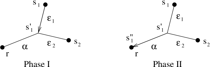
In Figure 9, we illustrate the motivation, in the case $k=2$, behind using T-theory to analyze the server problem. Let $\varepsilon_{{}_{1}}=\alpha_{{}_{{\left\{s_{1}\right\}},{\left\{s_{2},r\right\}}}}$, $\varepsilon_{{}_{2}}=\alpha_{{}_{{\left\{s_{2}\right\}},{\left\{s_{1},r\right\}}}}$, and $\alpha=\alpha_{{}_{{\left\{r\right\}},{\left\{s_{1},s_{2}\right\}}}}$. If $s_{{}_{i}}$ serves the request, the total distance it moves is $\varepsilon_{{}_{i}}+\alpha$. We can say that $\varepsilon_{{}_{i}}$ is the unique portion of that distance, while $\alpha$ is the common portion. When we make a decision as to which server to move, instead of comparing the two distances to $r$, we could compare the unique portions of those distances. In Figure 9, we assume that $s_{{}_{1}}$ serves the request at $r$. The movement of $s_{{}_{1}}$ can be thought of as consisting of two phases. During the first phase, $s_{{}_{1}}$ moves towards both points $r$ and $s_{{}_{2}}$. In the second phase, further movement towards both $r$ and $s_{{}_{2}}$ is impossible, so $s_{{}_{1}}$ moves towards $r$ and away from $s_{{}_{2}}$.

In the case that $k=2$, this intuition leads to modification of the Irani-Rubinfeld algorithm, balance2, [56] to balance slack, which we discuss in §5.2, and modification of harmonic [66] to random slack, which we discuss in §8.2. For $k>3$, the intuition is still present, but it is far less clear how to modify balance2 and harmonic to improve their competitivenesses. Teia [72] has partially succeeded; his algorithm handicap, discussed in this paper in Section 7, is a generalization of balance slack to all $k$. handicap is trackless, and is $k$-competitive against the lazy adversary for all $k$. Teia [72] also proves that, for $k=3$, handicap is 157-competitive against any adversary (Theorem 4 of this paper).

3 The Virtual Server Construction

In an arbitrary metric space $M$, the points to which we would like to move the servers may not exist. We overcome that restriction by allowing servers to virtually move in $T(M)$, while leaving the real servers in $M$. (In an implementation, the algorithm keeps the positions of the virtual servers in memory.)

More generally, if $M\subseteq M^{\prime}$ are metric spaces and there is a $C$-competitive online algorithm ${\cal A}^{\prime}$ for the $k$-server problem in $M^{\prime}$, there is a $C$-competitive online algorithm ${\cal A}$ for the $k$-server problem in $M$. If ${\cal A}^{\prime}$ is deterministic or randomized, ${\cal A}$ is deterministic or randomized, respectively. As requests are made, ${\cal A}$ makes use of ${\cal A}^{\prime}$ to calculate the positions the servers of ${\cal A}^{\prime}$, which we call virtual servers. When there is a request $r\in M$, ${\cal A}$ calculates the response of ${\cal A}^{\prime}$ and, in its memory, moves the virtual servers in $M^{\prime}$. If the $i^{\rm th}$ virtual server serves the request, then ${\cal A}$ moves the $i^{\rm th}$ real server in $M$ to $r$ to serve the request, but does not move any other real servers.

We give a formal description of the construction of ${\cal A}$ from ${\cal A}^{\prime}$:

 
Virtual Server Construction

• Let ${\left\{s_{{}_{i}}\right\}}$ be the servers in $M$, and let ${\left\{s^{\prime}_{{}_{i}}\right\}}$ be the virtual servers in $M^{\prime}$.

• Let $s^{\prime}_{{}_{i}}=s_{{}_{i}}$ for all $i$.

• Initialize ${\cal A}^{\prime}$.

• For each request $r$:

• • Move the virtual servers in $M^{\prime}$ according to the algorithm ${\cal A}^{\prime}$.

  • At least one virtual server will reach $r$. If $s^{\prime}_{{}_{i}}$ reaches $r$, move $s_{{}_{i}}$ to $r$. All other servers remain in their previous positions.

 

We can assume that the virtual servers match the real servers initially. If a server $s_{{}_{i}}$ serves request $r^{t}$ and then also serves request $r^{t^{\prime}}$, for some $t^{\prime}>t$, then $s_{{}_{i}}$ does not move during any intermediate step. The corresponding virtual server can make several moves between those steps, matching the real server at steps $t$ and $t^{\prime}$. Thus, by the triangle inequality, the movement of each virtual server is as least as great as the movement of the corresponding real server. Thus, ${\mbox{\it cost\/}}_{{}_{{\cal A}}}\leq{\mbox{\it cost\/}}_{{{}_{{\cal A}^{\prime}}}}$ for the entire request sequence. It follows that the competitiveness of ${\cal A}$ cannot exceed the the competitiveness of ${\cal A}^{\prime}$.

4 Tree Algorithms

The tree algorithm, which we call tree, a $k$-competitive online algorithm for the $k$-server problem in a tree, occupies a central place in the construction of a number of the online algorithms for the $k$-server problem presented in this paper. The line algorithm, Double Coverage, given in §4.1 below, is the direct ancestor of tree.

4.1 Double Coverage

In [25], Chrobak, Karloff, Payne, and Viswanathan defined a deterministic memoryless fast $k$-competitive online algorithm, called double coverage (DC), for the real line. If a request $r$ is to the left or right of all servers, the nearest server serves. If $r$ is between two servers, they both move toward the $r$ at the same speed and stop when one of them reaches $r$.

 
Double Coverage

• For each request $r$:

• • If $r$ is at the location of some server, serve $r$ at no cost.

  • If $r$ is to the left of all servers, move the leftmost server to $r$.

  • If $r$ is to the right of all servers, move the rightmost server to $r$.

  • If $s_{{}_{i}}<r<s_{{}_{j}}$ and there are no servers in the open interval ${\left(s_{{}_{i}},s_{{}_{j}}\right)}$, let $\delta=\min{\left\{r-s_{{}_{i}},s_{{}_{j}}-r\right\}}$. Move $s_{{}_{i}}$ to the right by $\delta$, and move $s_{{}_{j}}$ to the left by $\delta$. At least one of those two servers will reach $r$.

 

Figure 10: The DOUBLE COVERAGE algorithm

4.2 The Tree Algorithm

DC is generalized by Chrobak and Larmore in [29] to a deterministic memoryless fast $k$-competitive online algorithm, tree, for the $k$-server problem in a tree. We can then extend tree to any metric space which embeds in a tree, using the virtual server construction given in Section 3.

 
The Tree Algorithm

• Repeat the following loop until some server reaches $r$:

• • Define each server $s_{{}_{i}}$ to be blocked if there is some server $s_{{}_{j}}$ such that $d(s_{{}_{i}},r)=d(s_{{}_{i}},s_{{}_{j}})+d(s_{{}_{j}},r)$, and either $d(s_{{}_{j}},r)<d(s_{{}_{i}},r)$ or $j<i$. Any server that is not blocked is active.

  • For each $i\neq j$, let $\alpha_{{}_{i,j}}=\alpha_{{}_{{\left\{s_{i}\right\}},{\left\{s_{j},r\right\}}}}={\mbox{$\frac{1}{2}$}}{\left(d(s_{{}_{i}},r)+d(s_{{}_{i}},s_{{}_{j}})-d(s_{{}_{j}},r)\right)}$.

  • If there is only one active server, move it to $r$.

  • If there is more than one active server:

  • • Let $\delta$ be the minimum value of all $\alpha_{{}_{i,j}}$ for all choices of $i,j$ such that both $s_{{}_{i}}$ and $s_{{}_{j}}$ are active.

    • Move each active server a distance of $\delta$ toward $r$.

 

Figure 11: The phases of one step of TREE

Assume $M$ is a tree. If $s_{{}_{1}},\ldots,s_{{}_{k}}$ are the servers and $r$ is a request, we say that $s_{{}_{i}}$ is blocked by $s_{{}_{j}}$ if $d(s_{{}_{i}},r)=d(s_{{}_{i}},s_{{}_{j}})+d(s_{{}_{j}},r)$, and either $d(s_{{}_{j}},r)<d(s_{{}_{i}},r)$ or $j<i$. Any server that is not blocked by another server is active. The algorithm serves the request by moving the servers in a sequence of phases. During each phase, all active servers move the same distance towards $r$. A phase ends when either one server reaches $r$ or some previously active server becomes blocked. After at most $k$ phases, some server reaches $r$ and serves the request. Figure 11 illustrates an example step (consisting of three phases) of tree where $k=4$. The proof of $k$-competitiveness of tree makes use of the Coppersmith-Doyle-Raghavan-Snir potential [37], namely

$$\Phi_{CDRS}=\sum_{1\leq i<j\leq k}d(s_{{}_{i}},s_{{}_{j}})+2\sum_{1\leq i\leq k}d(s_{{}_{i}},a_{{}_{i}})$$

where ${\left\{a_{{}_{1}},\ldots,a_{{}_{k}}\right\}}$ is the set of positions of the optimal servers and ${\left\{s_{{}_{i}}\leftrightarrow a_{{}_{i}}\right\}}$ is the minimum matching of the algorithm servers with the optimal servers. We refer the reader to [29] for details of the proof.

More generally, if $M$ satisfies the four point condition given in Inequality (2), then $T(M)$ is a tree. We simply use the above algorithm on $T(M)$ to define a $k$-competitive algorithm on $M$, using the method of Section 3. We remark that in the original paper describing tree [29], there was no mention of the tight span construction. The result was simply stated using the clause, “If $M$ embeds in a tree ….”

4.3 The Slack Coverage Algorithm

Bartal’s Slack Coverage algorithm (SC) is 3-competitive for the 2-server problem in any Euclidean space [6].

 
Slack Coverage

• For each request $r$:

• • Without loss of generality, $d(s_{{}_{1}},r)\leq d(s_{{}_{2}},r)$.

  • Let $\delta=\alpha_{{}_{{\left\{s_{1}\right\}},{\left\{s_{2},r\right\}}}}={\mbox{$\frac{1}{2}$}}{\left(d(s_{{}_{1}},r)+d(s_{{}_{1}},s_{{}_{2}})-d(s_{{}_{2}},r)\right)}$.

  • Move $s_{{}_{1}}$ to $r$.

  • Move $s_{{}_{2}}$ a distance of $\delta$ along a straight line toward $r$.

 

Figure 12: One step of Bartal’s Slack Coverage algorithm in a Euclidean space: $s_{{}_{1}}$ serves, and $s_{{}_{2}}$ moves $\alpha_{{}_{{\left\{s_{1}\right\}},{\left\{s_{2},r\right\}}}}=7$ towards $r$

The intuition behind SC is that a Euclidean space $E$ is close to being injective. Figure 12 illustrates one step of SC. First, construct $T(X)$, where $X={\left\{s_{{}_{1}},s_{{}_{2}},r\right\}}$. In $X$, the response of the algorithm tree would be to move $s_{{}_{1}}$ to $r$ to serve the request, and to move $s_{{}_{2}}$ a distance of $\delta=\alpha_{{}_{{\left\{s_{1}\right\}},{\left\{s_{2},r\right\}}}}$ towards $r$, in $T(X)$. SC approximates that move by moving $s_{{}_{2}}$ that same distance in $E$ towards $r$. We refer the reader to pages 159–160 of [21] for the proof that SC is 3-competitive.

5 Balance Algorithms

Informally, we say that a server algorithm is a balance algorithm if it attempts, in some way, to balance the work among the servers. Three algorithms discussed in this paper satisfy that definition: balance2, balance slack, and handicap.

5.1 BALANCE2

The Irani-Rubinfeld algorithm, also called balance2 [56], tries to equalize the total movement of each server. More specifically, when there is a request $r$, balance2 chooses to move that server $s_{{}_{i}}$ which minimizes $C_{i}+2\cdot d(s_{{}_{i}},r)$, where $C_{i}$ is the total cost incurred by $s_{{}_{i}}$ on all previous moves. balance2 is trackless and needs $O(k)$ memory.

 
BALANCE2

• Let $C_{i}=0$ for all $i$

• For each request $r$:

• • Pick the $i$ which minimizes $C_{i}+2\cdot d(s_{{}_{j}},r)$.

  • $C_{i}=C_{i}+d(s_{{}_{i}},r)$.

  • Move $s_{{}_{i}}$ to $r$.

 

From [28] and [56] we have

Theorem 1

The competitiveness of balance2 for $k=2$ is at least 6 and at most 10.

The competitiveness of balance2 for $k>2$ is open.

5.2 BALANCE SLACK

Figure 13: Computing the moves for BALANCE SLACK and RANDOM SLACK

balance slack [28], defined only for $k=2$, is a modification of balance2. This algorithm tries to equalize the total slack work; namely, the sum, over all requests, of the Phase I costs, as illustrated in Figure 9.

 
BALANCE SLACK

• Let $e_{i}=0$ for $i=1,2$.

• For each request $r$:

• • $\varepsilon_{{}_{1}}=\alpha_{{\left\{s_{{}_{1}}\right\}},{\left\{s_{{}_{2}},r\right\}}}$

  • $\varepsilon_{{}_{2}}=\alpha_{{\left\{s_{{}_{2}}\right\}},{\left\{s_{{}_{1}},r\right\}}}$

  • Pick that $i$ which minimizes $e_{{}_{i}}+\varepsilon_{{}_{i}}$

  • $e_{{}_{i}}=e_{{}_{i}}+\varepsilon_{{}_{i}}$

  • Move $s_{{}_{i}}$ to $r$.

 

We associate each $s_{{}_{i}}$ with a number $e_{{}_{i}}$, the slack work, which is updated at each move. If $r$ is the request point, let $X={\left\{s_{{}_{1}},s_{{}_{2}},r\right\}}$, a 3-point subspace of $M$. Let $\varepsilon_{{}_{1}}=\alpha_{{\left\{s_{{}_{1}}\right\}},{\left\{s_{{}_{2}},r\right\}}}$ and $\varepsilon_{{}_{2}}=\alpha_{{\left\{s_{{}_{2}}\right\}},{\left\{s_{{}_{1}},r\right\}}}$, as shown in Figure 13. We now update the slack work values as follows. If $s_{{}_{i}}$ serves the request, we increment $e_{{}_{i}}$ by adding $\varepsilon_{{}_{i}}$, while the other slack work remains the same. We call $\varepsilon_{{}_{i}}$ the slack cost of the move if $s_{{}_{i}}$ serves the request. The algorithm balance slack then makes that choice which minimizes the value of $\max{\left\{e_{{}_{1}},e_{{}_{2}}\right\}}$ after the move.

balance slack is trackless, because it makes no use of any information regarding any point other than the distances between the three active points, namely the points of $X$, but it is not quite memoryless, as it needs to remember one number, viz, $e_{{}_{1}}-e_{{}_{2}}$.

From [28] we have

Theorem 2

balance slack is 4-competitive for $k=2$.

5.3 HANDICAP

Teia’s algorithm, handicap [72], is also a balance algorithm, a rather sophisticated generalization of balance slack. handicap is defined for all $k$ and all metric spaces, and is $k$-competitive against the lazy adversary. We postpone discussion of handicap until Section 7.

6 Server Algorithms in the Tight Span

The tight span algorithm, tree, and equipoise [26, 29, 32] permit movement of virtual servers in the tight span of the metric space. The purpose of using the tight span is that an algorithm might need to move servers to virtual points that do not exist in the original metric space. The tight span, due to the universal property described in §2.1, contains every virtual point that might be needed and no others.

6.1 Virtual Servers in the Tight Span

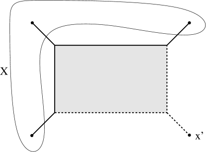
The tight span algorithm, tree, and equipoise [26, 29, 32], described in this paper in Sections 4 and 6, are derived using the embedding $M\subseteq T(M)$, from algorithms defined on $T(M)$. One problem with that derivation is that, in the worst case, $O({\left|M\right|})$ numbers are required to encode a point in $T(M)$, which is impossible if $M$ is infinite. Fortunately, we can shortcut the process by assuming the virtual servers are in the tight span of a finite space. If $X\subseteq X^{\prime}$ are metric spaces and $X^{\prime}=X\cup{\left\{x^{\prime}\right\}}$, there is a canonical embedding $\iota:T(X)\subseteq T(X^{\prime})$ where, for any $f\in T(X)$:

$$(\iota(f))(x)=\left\{\begin{array}[]{l}f(x){\ {\mbox{\rm if}}\ }x\in X\\ \sup_{y\in X}{\left\{d(x^{\prime},y)-f(y)\right\}}{\ {\mbox{\rm if}}\ }x=x^{\prime}\end{array}\right.$$

By an abuse of notation, we identify $f$ with $\iota(f)$. In Figure 14, $X$ consists of three points, and $T(X)$ is the union of the solid line segments, while $T(X^{\prime})$ is the entire figure, where $X^{\prime}=X\cup{\left\{x^{\prime}\right\}}$.

Figure 14: The inclusion $\iota:T(X)\subseteq T(X^{\prime})$ where ${\left|X\right|}=3$ and $X^{\prime}=X\cup{\left\{x^{\prime}\right\}}$

Continuing with the construction, let $s^{{\scriptscriptstyle 0}}_{{}_{1}},\ldots,s^{{\scriptscriptstyle 0}}_{k}\in M$ be the initial positions of the servers, and $r^{{\scriptscriptstyle 1}}\ldots r^{n}$ the request sequence. Let $X^{t}={\left\{s^{{\scriptscriptstyle 0}}_{{}_{1}},\ldots,s^{{\scriptscriptstyle 0}}_{{}_{k}},r^{1},\ldots,r^{t}\right\}}$, a set of cardinality of at most $k+t$, for $0\leq t\leq n$. Before the $t^{\rm th}$ request all virtual servers are in $T(X^{t-1})$.

Let ${\cal A}^{\prime}$ be an online algorithm for the $k$-server problem in $T(M)$ and ${\cal A}$ the algorithm in $M$ derived from ${\cal A}^{\prime}$ using the virtual server construction of Section 3. When the request $r{{}^{t}}$ is received, ${\cal A}$ uses the canonical embedding $T(X^{t-1})\subseteq T(X^{t})$ to calculate the positions of the virtual servers in $T(X^{t})$, then uses ${\cal A}^{\prime}$ to move the virtual servers within $T(X^{t})$. At most, ${\cal A}$ is required to remember the distance of each virtual server to each point in $X^{t}$.

6.2 The Tight Span Algorithm

tree of §4.2 generalizes to all metric spaces in the case that $k=2$, essentially because $T(X)$ is a tree for any metric space $X$ with at most three points. This generalization was first defined in [29], but was not named in that paper. We shall call it the tight span algorithm. As we did for tree, we first define the tight span algorithm as a fast memoryless algorithm in any injective metric space. We then use the virtual construction of Section 3 to extend the definition of the tight span algorithm to any metric space.

 
The Tight Span Algorithm

• For each request $r$:

• • Let $X={\left\{s_{{}_{1}},s_{{}_{2}},r\right\}}$.

  • Pick an embedding $T(X)\subseteq M$.

  • Execute tree on $T(X)$.

 

Assume that $M$ is injective, i.e., $M=T(M)$. We define the tight span algorithm on $M$ as follows: let $X={\left\{s_{{}_{1}},s_{{}_{2}},r\right\}}\subseteq M$. Since $M$ is injective, the inclusion $X\subseteq M$ can be extended to an embedding of $T(X)$ into $M$. Since $T(X)$ is a tree, use tree to move both servers in $T(X)$ such that one of the servers moves to $r$. Since $T(X)\subseteq M$, we can move the servers in $M$. In Figure 15, we show an example consisting of two steps of the tight span algorithm, where $M$ is the Manhattan plane.

Figure 15: The tight span algorithm in the Manhattan plane

Finally, we extend the tight span algorithm to an arbitrary metric space by using the virtual server construction given in Section 3. We refer the reader to [26] for the proof of 2-competitiveness for $k=2$, which also uses the Coppersmith-Doyle-Raghavan-Snir potential.

6.3 EQUIPOISE

Figure 16: One step of EQUIPOISE in the Manhattan plane
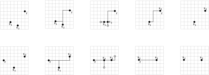
$\bullet$ Figure 16(a) shows the computation of $w_{{}_{12}}$.
$\bullet$ Figure 16(b) shows the computation of $w_{{}_{13}}$.
$\bullet$ Figure 16(c) shows the computation of $w_{{}_{23}}$.
$\bullet$ Figure 16(d) shows the weighted graph $G$.
$\bullet$ Figure 16(e) indicates $E_{MST}={\left\{e_{{}_{13}},e_{{}_{23}}\right\}}$, the minimum spanning tree of $G$.
$\bullet$ Figure 16(f) shows $T(X)$, with the two-dimensional cell of $T(X)$ shaded.
$\bullet$ Figure 16(g) shows $T_{e_{13}}$, and the position $s_{{}_{3}}$ would move to if tree for two servers were executed on $T_{e_{13}}$
$\bullet$ Figure 16(h) shows $T_{e_{23}}$, and the position $s_{{}_{2}}$ would move to if tree for two servers were executed on $T_{e_{23}}$.
$\bullet$ Figure 16(i) shows the minimum matching movement of $S$ to $S^{\prime}$.
$\bullet$ Figure 16(j) shows the positions of the three servers after completion of the step.

In [32], a deterministic algorithm for the $k$-server problem, called equipoise, is given. For $k=2$, equipoise is the tight span algorithm of [26] discussed in §6.2, and is 2-competitive. For $k=3$, equipoise is 11-competitive. The competitiveness of equipoise for $k\geq 4$ is unknown.

 
EQUIPOISE

• For each request $r$:

• • Let $G$ be the complete graph whose nodes are $S={\left\{s_{{}_{1}},\ldots,s_{{}_{k}}\right\}}$
    and whose edges are $E={\left\{e_{{}_{i,j}}\right\}}$.

  • For each $1\leq i<j\leq k$, let $w_{{}_{i,j}}=d(s_{{}_{i}},s_{{}_{j}})+d(s_{{}_{i}},r)+d(s_{{}_{j}},r)$ be the weight of $e_{{}_{i,j}}$.

  • Let $E_{MST}\subseteq E$ be the edges of a minimum spanning tree of $G$.

  • For each $e=e_{{}_{i,j}}\in E_{MST}$:

  • • Let $T_{e}$ be the tight span of ${\left\{s_{{}_{i}},s_{{}_{j}},r\right\}}$. Choose an embedding $T_{e}\subseteq M$.

    • Emulate tree on $T_{e}$ for two servers at $s_{{}_{i}}$ and $s_{{}_{j}}$ and request point $r$. One of those servers will move to $r$, while the other will move to some point $p_{e}\in T_{e}\subseteq M$.

  • Let $S^{\prime}={\left\{r\right\}}\cup{\left\{p_{e}\ |\ e\in E_{{}_{MST}}\right\}}$, a set of cardinality $k$.

  • Move the servers to $S^{\prime}$, using a minimum matching of $S$ and $S^{\prime}$. One server will move to $r$.

 

Let $M$ be an arbitrary metric space. We first define equipoise assuming that $M$ is injective. Let $S={\left\{s_{{}_{1}},\ldots,s_{{}_{k}}\right\}}$, the configuration of our servers in $M$, let $r$ be the request point, and let $X={\left\{s_{{}_{1}},\ldots,s_{{}_{k}},r\right\}}$. Let $G$ be the complete weighted graph whose vertices are $S$ and whose edge weights are ${\left\{w_{i,j}\right\}}$, where $w_{i,j}=d(s_{{}_{i}},s_{{}_{j}})+d(s_{{}_{i}},r)+d(s_{{}_{j}},r)$ for any $i\neq j$, Let $E_{{}_{MST}}$ be the set of edges of a minimum spanning tree for $G$.

For each $e=e_{{}_{i,j}}={\left\{s_{{}_{i}},s_{{}_{j}}\right\}}\in E_{{}_{MST}}$, let $X_{e}={\left\{s_{{}_{i}},s_{{}_{j}},r\right\}}$, and let $T_{e}=T(X_{e})$, and choose an embedding $T_{e}\subseteq M$. We then use the algorithm tree, for two servers, as a subroutine. For each $e=e_{{}_{i,j}}\in E_{MST}$, we consider how tree would serve the request $r$ if its two servers were at $s_{{}_{i}}$ and $s_{{}_{j}}$. It would move one of those servers to $r$, and the other to some other point in $M$, which we call $p_{e}$. Let $S^{\prime}={\left\{r\right\}}\cup{\left\{p_{e}\ |\ e\in E_{{}_{MST}}\right\}}$, a set of cardinality $k$. equipoise then serves the request at $r$ by moving its servers from $S$ to $S^{\prime}$, using the minimum matching of those two sets. One server will move to $r$, serving the request. Figure 16 shows one step of equipoise in the case $k=3$, where $M$ is the Manhattan plane. By using the virtual server construction of Section 3, we extend equipoise to all metric spaces.

7 Definition and Analysis of HANDICAP

In this section, we define the algorithm handicap, a generalization of balance slack, given initially in Teia’s dissertation [72], using slightly different notation. handicap is trackless and fast, but not memoryless.

The algorithm given in [27] is $k$-competitive against the lazy adversary, but only if the adversay is benevolent i.e., informs us when our servers matches his; handicap is more general, since it does not have that restriction.

For $k\leq 3$, handicap has the least competitiveness of any known deterministic trackless algorithm for the $k$-server problem. The competitiveness of handicap for $k\geq 4$ is unknown.

We give a proof that, for all $k$, handicap is $k$-competitive against the lazy adversary; in fact, against any adversary that can have at most one open server, i.e., a server in a position different from any of the algorithm’s servers. This result was proved in [72]. The proof given here is a simplification inspired by Teia [71].

7.1 Definition of HANDICAP

handicap maintains numbers $E_{1},\ldots,E_{k}$, where $E_{i}$ is called the handicap of the $i^{\rm th}$ server. The handicap of each server is updated after every step, and is used to decide which server moves. The larger a server’s handicap, the less likely it is to move. Since only the differences of the handicaps are used, the algorithm remembers only $k-1$ numbers between steps.

 
HANDICAP

• Let $E_{j}=0$ for all $j$

• For each request $r$:

• • Pick that $i$ for which $E_{i}+d(s_{{}_{i}},r)$ is minimized.

  • For all $1\leq j\leq k$:
     $E_{j}=E_{j}+\alpha_{{\left\{r\right\}},{\left\{s_{{}_{i}},s_{{}_{j}}\right\}}}$

  • Move $s_{{}_{i}}$ to $r$.

 

Initially, all handicaps are zero. At any step, let $s_{{}_{1}},\ldots,s_{{}_{k}}$ be the positions of our servers, and let $r$ be the request point. For all $1\leq i,j\leq k$, define $\alpha_{{}_{ij}}=\alpha_{{}_{\{r\},\{s_{{}_{i}},s_{{}_{j}}\}}}$, the isolation index. Choose that $i$ for which $E_{i}+d(s_{{}_{i}},r)$ is minimized, breaking ties arbitrarily. Next, update the handicaps by adding $\alpha_{{}_{ij}}$ to $E_{j}$ for each $j$, and then move the $i^{\rm th}$ server to $r$. The other servers do not move. It is a simple exercise to prove, for $k=2$, that handicap $\equiv$ balance slack. Simply verify that $e_{{}_{1}}-e_{{}_{2}}=E_{1}-E_{2}$, and that $e_{{}_{1}}+\varepsilon_{{}_{1}}\leq e_{{}_{2}}+\varepsilon_{{}_{2}}$ if and only if $E_{1}+d(s_{{}_{1}},r)\leq E_{2}+d(s_{{}_{2}},r)$.

Let $a_{{}_{1}},\ldots,a_{{}_{k}}$ be the adversary’s servers. We assume that the indices are assigned in such a way that ${\left\{s_{{}_{{}_{i}}}\leftrightarrow a_{{}_{{}_{i}}}\right\}}$ is a minimum matching. If $s_{{}_{i}}\neq a_{{}_{i}}$, we say that $s_{{}_{i}}\leftrightarrow a_{{}_{i}}$ is an open matching, and $a_{{}_{i}}$ is an open server. If $s_{{}_{i}}=a_{{}_{i}}$ for all $i$, we can arbitrarily designate any $a_{{}_{i}}$ to be the open server. We now prove that handicap is $k$-competitive against any adversary which may not have more than one open server, using the Teia potential defined below, a simplification of the potential used in [72].

Figure 17: Definitions of $\alpha_{ij}$ and $\varepsilon^{{}^{i}}_{{}_{j}}$ for handicap

7.2 Competitiveness of HANDICAP Against the Lazy Adversary

In order to aid the reader’s intuition, we define the Teia potential $\Phi$, to be a sum of simpler quantities.

$\begin{array}[]{rcl}{\mbox{\rm\bf Name}}&{\mbox{\rm\bf Notation}}&{\mbox{\rm{\bf Formula}}}\\ \rule{0.0pt}{14.45377pt}{\mbox{\rm Server Diversity}}&{\cal D}&\sum\limits_{1\leq i<j\leq k}d(s_{{}_{i}},s_{{}_{j}})\\ \rule{0.0pt}{21.68121pt}{\mbox{\rm$k\cdot$(Minimum Matching)}}&{\cal M}&k\cdot\sum\limits_{i=1}^{k}d(a_{{}_{i}},s_{{}_{i}})\\ \rule{0.0pt}{14.45377pt}{\mbox{\rm Coppersmith-Doyle-Raghavan-Snir Potential }}&\Phi_{CDRS}&{\cal D}+{\cal M}\\ \rule{0.0pt}{14.45377pt}{\mbox{\rm Tension ({\em Spannung}) Induced by $s_{{}_{i}}$ on ${\left\{a_{{}_{j}},s_{{}_{j}}\right\}}$}}&\varepsilon^{i}_{{}_{j}}&\alpha_{\{s_{{}_{j}}\},\{a_{{}_{j}},s_{{}_{i}}\}}{\ {\mbox{\rm for all}}\ }i,j\\ \rule{0.0pt}{21.68121pt}{\mbox{\rm Total Tension Induced by $s_{{}_{i}}$}}&\varepsilon^{i}&\sum\limits_{j=1}^{k}\varepsilon^{i}_{{}_{j}}{\ {\mbox{\rm for all}}\ }i\\ \rule{0.0pt}{14.45377pt}{\mbox{\rm Net Handicap of $s_{{}_{i}}$}}&e_{{}_{i}}&E_{i}-\varepsilon^{i}{\ {\mbox{\rm for all}}\ }i\\ \rule{0.0pt}{14.45377pt}{\mbox{\rm Maximum Net Handicap}}&e_{\max}&\max\limits_{{}_{1\leq i\leq k}}e_{{}_{i}}\\ \rule{0.0pt}{21.68121pt}{\mbox{\rm Handicap Portion of Potential}}&{\cal H}&2\cdot\sum\limits_{i=1}^{k}{\left(e_{\max}-E_{i}\right)}\\ \rule{0.0pt}{14.45377pt}{\mbox{\rm Teia Potential}}&\Phi&\Phi_{CDRS}+{\cal H}\end{array}$

We prove that $\Phi$ is non-negative, and that the following update condition holds for each step:

$$\Delta\Phi-k\cdot{\mbox{\it cost\/}}_{{}_{{\mbox{\it adv}}}}+{\mbox{\it cost\/}}_{{}_{{\mbox{\it alg}}}} \leq 0$$ (3)

where ${\mbox{\it cost\/}}_{{}_{{\mbox{\it alg}}}}$ and ${\mbox{\it cost\/}}_{{}_{{\mbox{\it adv}}}}$ are the algorithm’s and the adversary’s costs for the step, and where $\Delta\Phi$ is the change in potential during that step.

Lemma 2

$\Phi\geq 0$.

Proof: By all $i$:

$$2\varepsilon^{i}_{{}_{1}} = d(s_{{}_{1}},s_{{}_{i}})+d(s_{{}_{1}},a_{{}_{1}})-d(a_{{}_{1}},s_{{}_{i}})\hskip 36.135pt{\ {\mbox{\rm by Observation \ref{obs: isolation 3 points}}}\ }$$

$$\leq d(s_{{}_{1}},s_{{}_{i}})+d(s_{{}_{1}},a_{{}_{1}})$$

Thus 

$$\Phi = {\cal D}+{\cal M}+{\cal H}$$

$$= \sum\limits_{1\leq i<j\leq k}d(s_{{}_{i}},s_{{}_{j}})+\sum\limits_{1\leq i<j\leq k}d(s_{{}_{i}},s_{{}_{j}})+2\cdot\sum\limits_{i=1}^{k}{\left(e_{\max}-E_{i}\right)}$$

$$\geq \sum\limits_{i=1}^{k}d(s_{i},s_{1})+k\cdot d(a_{1},s_{1})+2\cdot\sum\limits_{i=1}^{k}{\left(e_{\max}-E_{i}\right)}$$

$$= \sum^{k}_{i=1}{\left(d(s_{{}_{1}},s_{{}_{i}})+d(s_{{}_{1}},a_{{}_{1}})+2{\left(e_{{}_{\max}}-e_{{}_{i}}-\varepsilon^{i}_{{}_{1}}\right)}\right)}$$

$$= \sum^{k}_{i=1}{\left({\left(d(s_{{}_{1}},s_{{}_{i}})+d(s_{{}_{1}},a_{{}_{1}})-2\varepsilon^{i}_{{}_{1}}\right)}+2{\left(e_{{}_{\max}}-e_{{}_{i}}\right)}\right)}$$

$$\geq 0$$

$\square$

Every step can be factored into a combination of two kinds of moves:

1. The adversary can move its open server to some other point, but make no request. We call this a cryptic move.

2. The adversary can request the position of its open server, without moving any server. We call this a lazy request.

To prove that Inequality (3), the update condition, holds for every step, it suffices to prove that it holds for every cryptic move and for every lazy request.

Lemma 3

Inequality (3) holds for a cryptic move.

Proof: We use the traditional $\Delta$ notation throughout to indicate the increase of any quantity.

Without loss of generality, $r=a_{{}_{1}}$, the open server. Let $\hat{a}_{{}_{1}}$ be the new position of the adversary’s server. Then $\Delta{\cal D}=0$, since the positions of the algorithm’s servers do not change, $\Delta{\cal M}=k\cdot{\left(d(s_{{}_{1}},\hat{a}_{{}_{1}})-d(s_{{}_{1}},a_{{}_{1}})\right)}$, and $\Delta e_{{}_{i}}=-\Delta\varepsilon_{{}_{1}}^{i}$ for each $i$. Since $\Delta e_{{}_{\max}}\leq\max_{i}\Delta e_{{}_{i}}$, there exists some $j$ such that

$$\Delta{\cal H} \leq -2k\cdot\Delta\varepsilon_{{}_{1}}^{j}$$

$$= k{\left(d(s_{{}_{1}},a_{{}_{1}})-d(a_{{}_{1}},s_{{}_{j}})-d(s_{{}_{1}},\hat{a}_{{}_{1}})+d(\hat{a}_{{}_{1}},s_{{}_{j}})\right)}\ \ {\mbox{\rm by Observation \ref{obs: isolation 3 points}}}$$

Thus 

$$\Delta\Phi-k\cdot{\mbox{\it cost\/}}_{{}_{{\mbox{\it adv}}}} = \Delta{\cal M}+\Delta{\cal H}-k\cdot d(a_{{}_{1}},\hat{a}_{{}_{1}})$$

$$\leq k{\left(d(\hat{a}_{{}_{1}},s_{{}_{j}})-d(a_{{}_{1}},s_{{}_{j}})-d(a_{{}_{1}},\hat{a}_{{}_{1}})\right)}$$

$$\leq 0$$

$\square$

Lemma 4

Inequality (3) holds for a lazy request.

Proof: Without loss of generality, $a_{{}_{1}}$ is the open server. Then $r=a_{{}_{1}}$, the request point.

Figure 18: Illustration of the proof of Lemma 4

Case I: $s_{{}_{1}}$ serves the request.

As illustrated in Figure 18, $\alpha_{{{}_{i}}{{}_{1}}}+\varepsilon^{i}_{{}_{1}}=d(s_{{}_{1}},a_{{}_{1}})$, for all $i$, $\Delta{\cal D}=\sum^{k}_{i=2}{\left(\alpha_{{{}_{i}}{{}_{1}}}-\varepsilon^{i}_{{}_{1}}\right)}$, and $\alpha_{{{}_{1}}{{}_{1}}}=d(s_{{}_{1}},a_{{}_{1}})$. Then

$$\Delta E_{i}\hskip 8.67204pt = \alpha_{{{}_{i}}{{}_{1}}}\rule{95.39693pt}{0.0pt}{\ {\mbox{\rm for all}}\ }i$$

$$\Delta e_{{}_{i}}\hskip 10.84006pt = \alpha_{{{}_{i}}{{}_{1}}}+\varepsilon^{i}_{{}_{1}}=d(s_{{}_{1}},a_{{}_{1}})\rule{18.7898pt}{0.0pt}{\ {\mbox{\rm for all}}\ }i$$

$$\Delta e_{{}_{\max}} = d(s_{{}_{1}},a_{{}_{1}})\rule{72.26999pt}{0.0pt}{\ {\mbox{\rm since}}\ }\min\Delta e_{{}_{i}}\leq\Delta e_{{}_{\max}}\leq\max\Delta e_{{}_{i}}$$

Thus 

$$\Delta\Phi+{\mbox{\it cost\/}}_{{}_{{\mbox{\it alg}}}} = \Delta{\cal D}+\Delta{\cal M}+\Delta{\cal H}+d(s_{{}_{1}},a_{{}_{1}})$$

$$= \sum^{k}_{i=2}{\left(\alpha_{{{}_{i}}{{}_{1}}}-\varepsilon^{i}_{{}_{1}}\right)}-k\cdot d(s_{{}_{1}},a_{{}_{1}})+2{\left(k\cdot d(s_{{}_{1}},a_{{}_{1}})-\sum^{k}_{i=1}\alpha_{{{}_{i}}{{}_{1}}}\right)}+d(s_{{}_{1}},a_{{}_{1}})$$

$$= (k+1)\cdot d(s_{{}_{1}},a_{{}_{1}})-\sum^{k}_{i=2}{\left(\alpha_{{{}_{i}}{{}_{1}}}+\varepsilon^{i}_{{}_{1}}\right)}-2\cdot\alpha_{{}_{11}}$$

$$= 0\ \ {\left({\ {\mbox{\rm since}}\ }\alpha_{{{}_{i}}{{}_{1}}}+\varepsilon^{i}_{{}_{1}}=d(s_{{}_{1}},a_{{}_{1}})=\alpha_{{}_{11}}\right)}$$

Case II: For some $i>1$, $s_{{}_{i}}$ serves the request. Without loss of generality, $i=2$. Using the carat notation to indicate the updated values after the move, we have $\hat{s}_{{}_{2}}=\hat{a}_{{}_{2}}=a_{{}_{1}}$, $\hat{s}_{{}_{1}}=a_{{}_{2}}$, $\hat{s}_{{}_{i}}=s_{{}_{i}}$ for all $i>2$, and $\hat{a}_{{}_{i}}=a_{{}_{i}}$ for all $i\neq 2$.

Claim A: $\Delta e_{{}_{i}}=\alpha_{{}_{12}}$ for all $i\neq 2$.

Using Observation 1:

$$e_{{}_{i}} = E_{i}-\varepsilon^{i}_{{}_{1}}$$

$$\hat{e}_{{}_{i}} = E_{i}+\alpha_{{}_{2i}}-\hat{\varepsilon}^{i}_{{}_{1}}$$

$$\varepsilon^{i}_{{}_{1}} = \frac{d(s_{{}_{i}},s_{{}_{1}})+d(s_{{}_{1}},a_{{}_{1}})-d(s_{{}_{i}},a_{{}_{1}})}{2}$$

$$\alpha_{{}_{2i}} = \frac{d(s_{{}_{2}},a_{{}_{1}})+d(s_{{}_{i}},a_{{}_{1}})-d(s_{{}_{2}},s_{{}_{i}})}{2}$$

$$\hat{\varepsilon}^{i}_{{}_{1}} = \frac{d(s_{{}_{i}},s_{{}_{1}})+d(s_{{}_{1}},a_{{}_{2}})-d(s_{{}_{i}},a_{{}_{2}})}{2}$$

$$\alpha_{{}_{12}} = \frac{d(s_{{}_{1}},a_{{}_{1}})+d(s_{{}_{2}},a_{{}_{1}})-d(s_{{}_{1}},s_{{}_{2}})}{2}$$

Combining the above equations, we obtain $\hat{e}_{{}_{i}}-e_{{}_{i}}-\alpha_{{}_{12}}=0$, which verifies Claim A.

Claim B: $\hat{e}_{{}_{\max}}=\hat{e}_{{}_{i}}$ for some $i\neq 2$.

Since handicap moves $s_{{}_{2}}$, we know that $E_{2}+d(s_{{}_{2}},a_{{}_{1}})\leq E_{1}+d(s_{{}_{1}},a_{{}_{1}})$.

$$\hat{e}_{{}_{1}} = \hat{E}_{1}+\alpha_{{}_{12}}=E_{1}+\alpha_{{}_{12}}\rule{72.26999pt}{0.0pt}{\ {\mbox{\rm by Claim A}}\ }$$

$$\hat{e}_{{}_{2}} = \hat{E}_{2}-\hat{\varepsilon}^{{\scriptscriptstyle 2}}_{{}_{1}}=E_{2}+d(s_{{}_{2}},a_{{}_{1}})-\hat{\varepsilon}^{{\scriptscriptstyle 2}}_{{}_{1}}$$

Thus 

$$\hat{e}_{{}_{1}}-\hat{e}_{{}_{2}} = E_{1}+\alpha_{{}_{12}}-E_{2}-d(s_{{}_{2}},a_{{}_{1}})+\hat{\varepsilon}^{{\scriptscriptstyle 2}}_{{}_{1}}\rule{144.54pt}{0.0pt}$$

$$\geq \alpha_{{}_{12}}-d(s_{{}_{1}},a_{{}_{1}})+\hat{\varepsilon}^{{\scriptscriptstyle 2}}_{{}_{1}}$$

$$= 0$$

Since $\hat{e}_{{}_{1}}\geq\hat{e}_{{}_{2}}$, we have verified Claim B.

We now continue with the proof of Case II of Lemma 4. From Claims A and B, $\Delta e_{{}_{\max}}\leq\alpha_{{}_{12}}$. Recall that $s_{{}_{2}}=a_{{}_{2}}$, and $r=a_{{}_{1}}$. Thus $\alpha_{{}_{22}}=\alpha_{{}_{\{r\},\{s_{{}_{2}},s_{{}_{2}}\}}}=d(s_{{}_{2}},a_{{}_{1}})$. Then

$$\Delta{\cal D} = \sum_{i\neq 2}{\left(d(s_{{}_{i}},a_{{}_{1}})-d(s_{{}_{i}},s_{{}_{2}})\right)}$$

$$\Delta{\cal M} = k{\left(d(s_{{}_{1}},a_{{}_{2}})-d(s_{{}_{1}},a_{{}_{1}})\right)}=k{\left(d(s_{{}_{1}},s_{{}_{2}})-d(s_{{}_{1}},a_{{}_{1}})\right)}$$

$$\Delta{\cal H} \leq 2k\cdot\alpha_{{}_{12}}-2\sum_{i=1}^{k}\alpha_{{}_{2i}}$$

$$\Delta\Phi+{\mbox{\it cost\/}}_{{}_{{\mbox{\it alg}}}} = \Delta{\cal D}+\Delta{\cal M}+\Delta{\cal H}+d(s_{{}_{2}},a_{{}_{1}})$$

$$\leq \sum_{i\neq 2}{\left(d(s_{{}_{i}},a_{{}_{1}})-d(s_{{}_{i}},s_{{}_{2}})\right)}+k{\left(d(s_{{}_{1}},s_{{}_{2}})-d(s_{{}_{1}},a_{{}_{1}})\right)}+2k\cdot\alpha_{{}_{12}}$$

$$\ \ \ \ -2\sum_{i=1}^{k}\alpha_{{}_{2i}}+d(s_{{}_{2}},a_{{}_{1}})$$

$$= k{\left(2\alpha_{{}_{12}}-d(s_{{}_{1}},a_{{}_{1}})+d(s_{{}_{1}},s_{{}_{2}})\right)}$$

$$\ \ \ \ -\sum_{i\neq 2}{\left(\alpha_{{}_{2i}}-d(s_{{}_{i}},a_{{}_{1}})+d(s_{{}_{i}},s_{{}_{2}})\right)}-2\alpha_{{}_{22}}+d(s_{{}_{2}},a_{{}_{1}})$$

$$= kd(s_{{}_{2}},a_{{}_{1}})-(k-1)d(s_{{}_{2}},a_{{}_{1}})-2d(s_{{}_{2}},a_{{}_{1}})+d(s_{{}_{2}},a_{{}_{1}})$$

$$= 0$$

This completes the proof of Lemma 4, since the left-hand side of the update condition is less than or equal to zero. $\square$

Theorem 3

handicap is $k$-competitive against any adversary which can have at most one open server.

Proof: Lemma 2 states that the Teia potential is non-negative, while Lemmas 3 and 4 state that the update condition, Inequality (3), holds for every step. $\square$

Teia also obtains a competitiveness of handicap against any adversary, for $k=3$. From Subsection 8.4 of Teia’s dissertation [72], on page 59:

Theorem 4

For $k=3$, handicap is 157-competitive.

8 Harmonic Algorithms

In this section, we present the classical algorithm harmonic, as well as random slack, an improvement of harmonic which uses T-theory. In §8.3 we present a T-theory based proof that harmonic is 3-competitive for $k=2$.

8.1 HARMONIC

harmonic is a memoryless randomized algorithm for the $k$-server problem, first defined by Raghavan and Snir [66, 67]. harmonic is based on the intuition that it should be less likely to move a larger distance than a smaller. harmonic moves each server with a probability that is inversely proportional to its distance to the request point.

 
HARMONIC

• For each request $r$:

• • For each $1\leq i\leq k$, let

    $$p_{{}_{i}} = \frac{\frac{1}{d(s_{{}_{i}},r)}}{\frac{1}{d(s_{{}_{1}},r)}+\cdots+\frac{1}{d(s_{{}_{k}},r)}}\rule{86.72377pt}{0.0pt}$$ (4)

  • Pick one $i$, where each $i$ is picked with probability $p_{i}$.

  • Move $s_{{}_{i}}$ to $r$.

 

harmonic is known to be 3-competitive for $k=2$ [30, 35]. Raghavan and Snir [66, 67] prove that its competitiveness cannot be less than ${\left(k+1\atop 2\right)}$, which is greater than the best known deterministic competitiveness of the $k$-server problem [63, 64]. For $k>2$, the true competitiveness of harmonic is unknown but finite [51]. harmonic is of interest because it is simple to implement.

8.2 RANDOM SLACK

random slack, defined only for two servers, is derived from harmonic, but moves each server with a probability inversely proportional to the unique distance that a server would move to serve the request, namely the Phase I cost (see Figure 9.)

 
RANDOM SLACK

• For each request $r$:

• • $\varepsilon_{{}_{1}}=\alpha_{{\left\{s_{{}_{1}}\right\}},{\left\{s_{{}_{2}},r\right\}}}$

  • $\varepsilon_{{}_{2}}=\alpha_{{\left\{s_{{}_{2}}\right\}},{\left\{s_{{}_{1}},r\right\}}}$

  • Let $p_{{}_{1}}=\frac{\varepsilon_{{}_{1}}}{\varepsilon_{{}_{1}}+\varepsilon_{{}_{2}}}$

  • Let $p_{{}_{2}}=\frac{\varepsilon_{{}_{2}}}{\varepsilon_{{}_{1}}+\varepsilon_{{}_{2}}}$

  • Pick one $i$, where each $i$ is picked with probability $p_{i}$.

  • Move $s_{{}_{i}}$ to $r$.

 

We refer the reader to [28] for the proof that random slack is 2-competitive.

8.3 Analysis of HARMONIC using Isolation Indices

The original proof that harmonic is 3-competitive for $k=2$ used T-theory, but was never published. In this section, we present an updated version of that unpublished proof.

We will first show that the lazy potential $\Phi$, defined below, satisfies an update condition for every possible move. In a manner similar to that in the proof of Theorem 3, we first factor all moves into three kinds, which we call active, lazy, and cryptic. After each step, harmonic’s two servers are located at points $s_{{}_{1}}$ and $s_{{}_{2}}$, and the adversary’s servers are located at points $a_{{}_{1}}$ and $a_{{}_{2}}$. Without loss of generality, $s_{{}_{2}}=a_{{}_{2}}$ is the last request point. In the next step, the adversary moves a server to a point $r$ and makes a request at $r$, and then harmonic moves one of its two servers to $r$, using the probability distribution given in Equation (4). We analyze the problem by requiring that the adversary always do one of three things:

1. Move the server at $a_{{}_{2}}$ to a new point $r$, and then request $r$. We call this an active request.

2. Request $a_{{}_{1}}$ without moving a server. We call this a lazy request.

3. Move the server from $a_{{}_{1}}$ to some other point, but make no request. We call this a cryptic move.

If the adversary moves its server from $a_{{}_{1}}$ to a new point $r$ and then requests $r$, we consider that step to consist of two moves: a cryptic move followed by a lazy request. Our analysis will be simplified by this factorization.

If $x,y,z\in M$, we define $\Phi(x,y,z)$, the lazy potential, to be the expected cost that harmonic will pay if $x=s_{{}_{1}}$, $y=a_{{}_{1}}$, and $z=s_{{}_{2}}=a_{{}_{2}}$, providing the adversary makes only lazy requests henceforth. The formula for $\Phi$ is obtained by solving the following two simultaneous equations:

$$\Phi(x,y,z) = \frac{2\cdot d(x,y)\cdot d(y,z)}{d(x,y)+d(y,z)}+\frac{d(x,y)}{d(x,y)+d(y,z)}\cdot\Phi(x,z,y)$$ (5)

$$\Phi(x,z,y) = \frac{2\cdot d(x,z)\cdot d(y,z)}{d(x,z)+d(y,z)}+\frac{d(x,z)}{d(x,z)+d(y,z)}\cdot\Phi(x,y,z)$$ (6)

Obtaining the solution

$$\Phi(x,y,z) = \frac{2\cdot d(x,y)(2\cdot d(x,z)+d(y,z))}{d(x,y)+d(x,z)+d(y,z)}$$ (7)

Theorem 5

harmonic is 3-competitive for 2 servers.

Proof: We will show that the lazy potential is 3-competitive. For each move, we need to verify the update condition, namely that the value of $\Phi$ before the move, plus three times the distance moved by the adversary server, is at least as great as the expected distance moved by harmonic plus the expected value of $\Phi$ after the move. The update condition holds for every lazy request, by Equation (5). We need to verify the update inequalities for active requests and cryptic moves.

If harmonic has servers at $x$ and $z$ and the adversary has servers at $y$ and $z$, the update condition for the active request where the adversary moves the server from $z$ to $r$ is:

$$\Phi(x,y,z)+3\cdot d(z,r)-\frac{2\cdot d(x,r)\cdot d(z,r)}{d(x,r)\cdot d(z,r)}-\frac{d(x,r)}{d(x,r)\cdot d(z,r)}\cdot\Phi(x,y,r)-\frac{d(z,r)}{d(x,r)\cdot d(z,r)}\cdot\Phi(z,y,r) \geq 0$$ (8)

If harmonic has servers at $x$ and $z$ and the adversary has servers at $y$ and $z$, the update condition for the cryptic move where the adversary moves the server from $y$ to $r$ is:

$$\Phi(x,y,z)+3\cdot d(y,r)-\Phi(x,r,z) \geq 0$$ (9)

Let $X={\left\{x,y,z,r\right\}}$. It will be convenient to choose a variable name for the isolation index of each split of $X$. Let:

$$a = \alpha_{{\left\{x\right\}},{\left\{y,z,r\right\}}}$$

$$b = \alpha_{{\left\{y\right\}},{\left\{x,z,r\right\}}}$$

$$c = \alpha_{{\left\{z\right\}},{\left\{x,y,r\right\}}}$$

$$d = \alpha_{{\left\{r\right\}},{\left\{x,y,z\right\}}}$$

$$e = \alpha_{{\left\{x,y\right\}},{\left\{z,r\right\}}}$$

$$f = \alpha_{{\left\{x,z\right\}},{\left\{y,r\right\}}}$$

$$g = \alpha_{{\left\{x,r\right\}},{\left\{y,z\right\}}}$$

By Lemma 1 and Observation 2, we have

$$d(x,y) = a+b+f+g$$

$$d(x,z) = a+c+e+g$$

$$d(y,z) = b+c+e+f$$

$$d(x,r) = a+d+e+f$$

$$d(y,r) = b+d+e+g$$

$$d(z,r) = c+d+f+g$$

Figure 19: Three possible pictures of the tight span of $X$

The three non-trivial splits of $X$ do not form a coherent set; thus, at least one of their isolation indices must be zero. Figure 19 shows the three generic possibilities for $T(X)$. Let $MaxMatch=\max{\left\{d(x,y)+d(z,r),d(x,z)+d(y,r),d(x,r)+d(y,z)\right\}}$. If $MaxMatch=d(x,y)+d(z,r)$, then $e=0$, as shown in Figure 19(a). If $MaxMatch=d(x,z)+d(y,r)$, then $f=0$, as shown in Figure 19(b). If $MaxMatch=d(x,r)+d(y,z)$, then $g=0$, as shown in Figure 19(c). In any case, the product $efg$ must be zero. Substituting the formula for each distance, and using the fact that $efg=0$, we compute the left hand side of Inequality (8) to be

$$\frac{{\mbox{\it numerator}}_{{}_{1}}}{(a+b+c+e+f+g)(a+b+d+e+f+g)(b+c+d+e+f+g)(a+c+2d+e+2f+g)}$$

where numerator${}_{{}_{1}}$ is a polynomial in the literals $a,b,c,d,e,f,$ and $g$, given in Appendix A.

Similarly, the left hand side of Inequality (9) is

$$\frac{{\mbox{\it numerator}}_{{}_{2}}}{(a+b+c+e+f+g)(a+c+d+e+f+g)}$$

where numerator${}_{{}_{2}}$ is also a polynomial in the literals $a,b,c,d,e,f,$ and $g$, given in Appendix A.

The denominators of these rational expressions are clearly positive. The proof that ${\mbox{\it numerator}}_{{}_{1}}$ and ${\mbox{\it numerator}}_{{}_{2}}$ are non-negative is given in Appendix A. Thus, the left hand sides of both inequalities are non-negative, thus verifying that harmonic is 3-competitive for two servers. $\square$

9 Summary and Possible Future Applications of T-Theory to the k-Server Problem

We have demonstrated the usefulness of T-theory for defining online algorithms for the server problem in a metric space $M$, and proving competitiveness by rewriting the update conditions in terms of isolation indices. In this section, we suggest ways to extend the use of T-theory to obtain new results for the server problem.

9.1 Using T-Theory to Generalize RANDOM SLACK

A memoryless trackless randomized algorithm for the $k$-server problem must act as follows. Given that the servers are at ${\left\{s_{{}_{1}}\ldots,s_{{}_{k}}\right\}}$ and the request is $r$, first compute $T(X)$, where $X={\left\{s_{{}_{1}}\ldots,s_{{}_{k}},r\right\}}$ and then use the parameters of $T(X)$ to compute the probabilities of serving the request with the various servers.

We know that this approach is guaranteed to yield a competitive memoryless randomized algorithm for the $k$-server problem, since harmonic is in this class. harmonic computes probabilities using the parameters of $T(X)$, but we saw in random slack in §8.2 that, for $k=2$, a more careful choice of probabilities yields an improvement of the competitiveness. We conjecture that, for $k\geq 3$, there is some choice of probabilities which yields an algorithm of this class whose competitiveness is lower than that of harmonic.

9.2 Using T-Theory to Analyze HARMONIC for Larger $k$

We know that the competitiveness of harmonic for $k=3$ is at least ${\left(4\atop 2\right)}=6$ [66, 67]. As in Section 8, we could express the lazy potential in closed form, and then attempt to prove that it satisfies all necessary update conditions.

In principle, the process of verifying that the lazy potential suffices to prove 6-competitiveness for harmonic for $k=3$ could be automated, possibly using the output of Sturmfels and Yu’s program [70] as input. However, the complexity of the proof technique used in Section 8 rises very rapidly with $k$, and may be impractical for $k>2$. There should be some way to simplify this computation.

9.3 Generalizing the Virtual Server Algorithms and the $k$-Server Conjecture

The $k$-server conjecture remains open, despite years of effort by many researchers. The most promising approach to date appears to be the effort to prove that the work function algorithm (WFA) [31], or perhaps a variant of WFA, is $k$-competitive. This opinion is explained in depth by Koutsoupias [61]. To date, for $k\geq 3$, it is only known that WFA is $(2k-1)$-competitive [64], and that it is $k$-competitive in a number of special cases.

handicap represents a somewhat different approach to the $k$-server problem. Teia conjectures that handicap can be modified in such a way as to obtain a 3-competitive deterministic online algorithm for the 3-server problem against an arbitrary adversary, thus settling the server conjecture for $k=3$. He suggests that this can be done by maintaining two reference points in the tight span. The resulting algorithm would not be trackless.

From the introduction (pp. 3–4) of Teia’s dissertation [72]:

For the case of more than one open matching, the memory representation would have to be augmented by additional components. One possibility would be to introduce reference points in addition to handicaps. We are convinced that, for $k=3$, by careful case analysis and the introduction of two reference points, a 3-competitive algorithm can be given.

Original German text:

Für den Fall mehr als eines offenen Matchings müßte die Gedächtnisrepräsentation um zusätzliche Komponenten erweitert werden. Eine Möglichkeit wäre, zusätzlich zu den Handicaps Bezugspunkte einzuführen. Wir sind überzeugt, daß sich für $k=3$ durch sorgfältige Fallunterscheidungen und die Einführung zweier Bezugspunkte ein 3- kompetitiver Algorithmus angeben läßt.

Appendix A Appendix: Mathematica Calculations

We used Mathematica 5.2 to rewrite the left hand side of Inequality (8) as a single rational expression with the least common denominator. We then substituted zero for $efg$ throughout. Then numerator${}_{{}_{1}}$, the numerator of the resulting rational expression, is the following polynomial: $4a^{3}bc+9a^{2}b^{2}c+5ab^{3}c+4a^{3}c^{2}+14a^{2}bc^{2}+13ab^{2}c^{2}+3b^{3}c^{2}+5a^{2}c^{3}+9abc^{3}+4b^{2}c^{3}+ac^{4}+bc^{4}+2a^{3}bd+3a^{2}b^{2}d+ab^{3}d+6a^{3}cd+23a^{2}bcd+24ab^{2}cd+7b^{3}cd+17a^{2}c^{2}d+36abc^{2}d+17b^{2}c^{2}d+10ac^{3}d+9bc^{3}d+c^{4}d+2a^{3}d^{2}+7a^{2}bd^{2}+5ab^{2}d^{2}+18a^{2}cd^{2}+37abcd^{2}+17b^{2}cd^{2}+21ac^{2}d^{2}+20bc^{2}d^{2}+5c^{3}d^{2}+6a^{2}d^{3}+10abd^{3}+4b^{2}d^{3}+16acd^{3}+16bcd^{3}+8c^{2}d^{3}+4ad^{4}+4bd^{4}+4cd^{4}+4a^{3}ce+17a^{2}bce+17ab^{2}ce+4b^{3}ce+13a^{2}c^{2}e+26abc^{2}e+11b^{2}c^{2}e+7ac^{3}e+6bc^{3}e+c^{4}e+2a^{3}de+9a^{2}bde+7ab^{2}de+25a^{2}cde+50abcde+21b^{2}cde+30ac^{2}de+26bc^{2}de+7c^{3}de+10a^{2}d^{2}e+18abd^{2}e+6b^{2}d^{2}e+37acd^{2}e+34bcd^{2}e+16c^{2}d^{2}e+14ad^{3}e+14bd^{3}e+14cd^{3}e+4d^{4}e+8a^{2}ce^{2}+16abce^{2}+6b^{2}ce^{2}+10ac^{2}e^{2}+7bc^{2}e^{2}+2c^{3}e^{2}+6a^{2}de^{2}+10abde^{2}+2b^{2}de^{2}+22acde^{2}+17bcde^{2}+9c^{2}de^{2}+12ad^{2}e^{2}+10bd^{2}e^{2}+13cd^{2}e^{2}+6d^{3}e^{2}+4ace^{3}+2bce^{3}+c^{2}e^{3}+4ade^{3}+2bde^{3}+3cde^{3}+2d^{2}e^{3}+2a^{3}bf+4a^{2}b^{2}f+2ab^{3}f+6a^{3}cf+30a^{2}bcf+33ab^{2}cf+8b^{3}cf+22a^{2}c^{2}f+46abc^{2}f+21b^{2}c^{2}f+13ac^{3}f+12bc^{3}f+c^{4}f+4a^{3}df+16a^{2}bdf+13ab^{2}df+2b^{3}df+39a^{2}cdf+88abcdf+43b^{2}cdf+54ac^{2}df+54bc^{2}df+13c^{3}df+16a^{2}d^{2}f+29abd^{2}f+10b^{2}d^{2}f+59acd^{2}f+59bcd^{2}f+31c^{2}d^{2}f+18ad^{3}f+16bd^{3}f+24cd^{3}f+4d^{4}f+2a^{3}ef+9a^{2}bef+8ab^{2}ef+b^{3}ef+30a^{2}cef+67abcef+30b^{2}cef+41ac^{2}ef+39bc^{2}ef+10c^{3}ef+20a^{2}def+41abdef+14b^{2}def+90acdef+85bcdef+45c^{2}def+42ad^{2}ef+39bd^{2}ef+58cd^{2}ef+22d^{3}ef+5a^{2}e^{2}f+9abe^{2}f+2b^{2}e^{2}f+30ace^{2}f+26bce^{2}f+15c^{2}e^{2}f+26ade^{2}f+21bde^{2}f+37cde^{2}f+23d^{2}e^{2}f+3ae^{3}f+be^{3}f+6ce^{3}f+7de^{3}f+2a^{3}f^{2}+10a^{2}bf^{2}+10ab^{2}f^{2}+2b^{3}f^{2}+23a^{2}cf^{2}+57abcf^{2}+28b^{2}cf^{2}+35ac^{2}f^{2}+35bc^{2}f^{2}+8c^{3}f^{2}+16a^{2}df^{2}+32abdf^{2}+12b^{2}df^{2}+70acdf^{2}+74bcdf^{2}+40c^{2}df^{2}+28ad^{2}f^{2}+24bd^{2}f^{2}+46cd^{2}f^{2}+12d^{3}f^{2}+11a^{2}ef^{2}+25abef^{2}+10b^{2}ef^{2}+57acef^{2}+58bcef^{2}+31c^{2}ef^{2}+44adef^{2}+41bdef^{2}+74cdef^{2}+37d^{2}ef^{2}+14ae^{2}f^{2}+12be^{2}f^{2}+26ce^{2}f^{2}+26de^{2}f^{2}+4e^{3}f^{2}+6a^{2}f^{3}+14abf^{3}+6b^{2}f^{3}+29acf^{3}+32bcf^{3}+17c^{2}f^{3}+20adf^{3}+18bdf^{3}+38cdf^{3}+14d^{2}f^{3}+17aef^{3}+17bef^{3}+32cef^{3}+27def^{3}+10e^{2}f^{3}+6af^{4}+6bf^{4}+12cf^{4}+8df^{4}+8ef^{4}+2f^{5}+4a^{3}bg+8a^{2}b^{2}g+4ab^{3}g+8a^{3}cg+34a^{2}bcg+33ab^{2}cg+6b^{3}cg+23a^{2}c^{2}g+45abc^{2}g+19b^{2}c^{2}g+13ac^{3}g+12bc^{3}g+c^{4}g+6a^{3}dg+24a^{2}bdg+23ab^{2}dg+6b^{3}dg+47a^{2}cdg+102abcdg+49b^{2}cdg+58ac^{2}dg+57bc^{2}dg+13c^{3}dg+23a^{2}d^{2}g+44abd^{2}g+18b^{2}d^{2}g+67acd^{2}g+66bcd^{2}g+33c^{2}d^{2}g+22ad^{3}g+20bd^{3}g+26cd^{3}g+4d^{4}g+4a^{3}eg+17a^{2}beg+16ab^{2}eg+3b^{3}eg+34a^{2}ceg+71abceg+30b^{2}ceg+42ac^{2}eg+39bc^{2}eg+10c^{3}eg+28a^{2}deg+57abdeg+22b^{2}deg+100acdeg+93bcdeg+46c^{2}deg+51ad^{2}eg+47bd^{2}eg+61cd^{2}eg+24d^{3}eg+9a^{2}e^{2}g+17abe^{2}g+6b^{2}e^{2}g+32ace^{2}g+27bce^{2}g+14c^{2}e^{2}g+30ade^{2}g+24bde^{2}g+37cde^{2}g+24d^{2}e^{2}g+5ae^{3}g+3be^{3}g+5ce^{3}g+6de^{3}g+6a^{3}fg+31a^{2}bfg+32ab^{2}fg+7b^{3}fg+55a^{2}cfg+125abcfg+56b^{2}cfg+72ac^{2}fg+69bc^{2}fg+16c^{3}fg+47a^{2}dfg+99abdfg+44b^{2}dfg+162acdfg+167bcdfg+84c^{2}dfg+76ad^{2}fg+69bd^{2}fg+102cd^{2}fg+28d^{3}fg+26a^{2}f^{2}g+62abf^{2}g+28b^{2}f^{2}g+99acf^{2}g+103bcf^{2}g+52c^{2}f^{2}g+86adf^{2}g+83bdf^{2}g+128cdf^{2}g+55d^{2}f^{2}g+34af^{3}g+35bf^{3}g+53cf^{3}g+45df^{3}g+14f^{4}g+4a^{3}g^{2}+19a^{2}bg^{2}+18ab^{2}g^{2}+3b^{3}g^{2}+31a^{2}cg^{2}+65abcg^{2}+26b^{2}cg^{2}+37ac^{2}g^{2}+34bc^{2}g^{2}+8c^{3}g^{2}+30a^{2}dg^{2}+64abdg^{2}+30b^{2}dg^{2}+92acdg^{2}+93bcdg^{2}+45c^{2}dg^{2}+48ad^{2}g^{2}+45bd^{2}g^{2}+57cd^{2}g^{2}+16d^{3}g^{2}+20a^{2}eg^{2}+43abeg^{2}+17b^{2}eg^{2}+67aceg^{2}+63bceg^{2}+33c^{2}eg^{2}+70adeg^{2}+66bdeg^{2}+87cdeg^{2}+49d^{2}eg^{2}+22ae^{2}g^{2}+19be^{2}g^{2}+28ce^{2}g^{2}+32de^{2}g^{2}+5e^{3}g^{2}+33a^{2}fg^{2}+76abfg^{2}+33b^{2}fg^{2}+109acfg^{2}+107bcfg^{2}+53c^{2}fg^{2}+110adfg^{2}+109bdfg^{2}+143cdfg^{2}+68d^{2}fg^{2}+64af^{2}g^{2}+65bf^{2}g^{2}+86cf^{2}g^{2}+86df^{2}g^{2}+35f^{3}g^{2}+13a^{2}g^{3}+28abg^{3}+11b^{2}g^{3}+39acg^{3}+36bcg^{3}+18c^{2}g^{3}+44adg^{3}+44bdg^{3}+53cdg^{3}+27d^{2}g^{3}+31aeg^{3}+29beg^{3}+39ceg^{3}+46deg^{3}+15e^{2}g^{3}+50afg^{3}+49bfg^{3}+61cfg^{3}+69dfg^{3}+41f^{2}g^{3}+14ag^{4}+13bg^{4}+16cg^{4}+20dg^{4}+15eg^{4}+23fg^{4}+5g^{5}$

Each of the variables $a,b,c,d,e,f,g$ is an isolation index, hence cannot be negative. Since there are no negative coefficients in the polynomial $numerator_{{}_{1}}$, its value must be non-negative.

Similarly, we used Mathematica to find a polynomial expression for $numerator_{{}_{2}}$, the numerator of the left hand side of Inequality (9): $4a^{2}b+4ab^{2}+9abc+4b^{2}c+6bc^{2}+2a^{2}d+6abd+4b^{2}d+3acd+6bcd+2ad^{2}+2bd^{2}+2cd^{2}+2a^{2}e+11abe+4b^{2}e+2ace+12bce+6ade+9bde+3cde+2d^{2}e+3ae^{2}+7be^{2}+ce^{2}+3de^{2}+e^{3}+8abf+4b^{2}f+8bcf+4adf+6bdf+4cdf+2d^{2}f+5aef+11bef+3cef+7def+4e^{2}f+4bf^{2}+2df^{2}+3ef^{2}+4a^{2}g+12abg+4b^{2}g+10acg+15bcg+6c^{2}g+7adg+9bdg+6cdg+2d^{2}g+12aeg+15beg+12ceg+9deg+7e^{2}g+7afg+11bfg+9cfg+7dfg+3f^{2}g+9ag^{2}+9bg^{2}+11cg^{2}+5dg^{2}+11eg^{2}+8fg^{2}+5g^{3}$ Every term is non-negative, hence $numerator_{{}_{2}}$ is non-negative.

References

- [1] Noga Alon, Richard M. Karp, David Peleg, and Douglas West. A graph-theoretic game and its application to the k-server problem. SIAM J. Comput., 24:78–100, 1995.
- [2] Ganesh R. Baliga and Anil M. Shende. On space bounded server algorithms. In Proc. 5th International Conference on Computing and Information, pages 77–81. IEEE, 1993.
- [3] Hans-Jürgen Bandelt and Victor Chepoi. Embedding metric spaces in the rectilinear plane: a six-point criterion. GEOMETRY: Discrete & Computational Geometry, 15:107–117, 1996.
- [4] Hans-Jürgen Bandelt and Victor Chepoi. Embedding into the rectilinear grid. NETWORKS: Networks: An International Journal, 32:127–132, 1998.
- [5] Hans-Jürgen Bandelt and Andreas Dress. A canonical decomposition theory for metrics on a finite set. Adv. Math., 92:47–105, 1992.
- [6] Yair Bartal. A fast memoryless 2-server algorithm in Euclidean spaces, 1994. Unpublished manuscript.
- [7] Yair Bartal, Marek Chrobak, and Lawrence L. Larmore. A randomized algorithm for two servers on the line. In Proc. 6th European Symp. on Algorithms (ESA), Lecture Notes in Comput. Sci., pages 247–258. Springer, 1998.
- [8] Yair Bartal, Marek Chrobak, and Lawrence L. Larmore. A randomized algorithm for two servers on the line. Inform. and Comput., 158:53–69, 2000.
- [9] Yair Bartal, Marek Chrobak, John Noga, and Prabhakar Raghavan. More on random walks, electrical networks, and the harmonic -server algorithm. Inform. Process. Lett., 84:271–276, 2002.
- [10] Yair Bartal and Edward Grove. The harmonic -server algorithm is competitive. J. ACM, 47(1):1–15, 2000.
- [11] Yair Bartal and Elias Koutsoupias. On the competitive ratio of the work function algorithm for the -server problem. Theoret. Comput. Sci., 324:337–345, 2004.
- [12] Yair Bartal and Manor Mendel. Randomized -server algorithms for growth-rate bounded graphs. In Proc. 15th Symp. on Discrete Algorithms (SODA), pages 666–671. ACM/SIAM, 2004.
- [13] Yair Bartal and Adi Rosén. The distributed -server problem — a competitive distributed translator for -server algorithms. In Proc. 33rd Symp. Foundations of Computer Science (FOCS), pages 344–353. IEEE, 1992.
- [14] Jean-Pierre Barthélemy and Alain Guénoche. Trees and Proximity Relations,. Wiley, Chichester, 1991. Translated from the French by Gregor Lawden.
- [15] Wolfgang Bein, Marek Chrobak, and Lawrence L. Larmore. The 3-server problem in the plane. In Proc. 7th European Symp. on Algorithms (ESA), volume 1643 of Lecture Notes in Comput. Sci., pages 301–312. Springer, 1999.
- [16] Wolfgang Bein, Marek Chrobak, and Lawrence L. Larmore. The 3-server problem in the plane. Theoret. Comput. Sci., 287:387–391, 2002.
- [17] Wolfgang Bein and Lawrence L. Larmore. Trackless online algorithms for the server problem. Inform. Process. Lett., 74:73–79, 2000.
- [18] Piotr Berman, Howard Karloff, and Gabor Tardos. A competitive algorithm for three servers. In Proc. 1st Symp. on Discrete Algorithms (SODA), pages 280–290. ACM/SIAM, 1990.
- [19] Avrim Blum, Howard Karloff, Yuval Rabani, and Michael Saks. A decomposition theorem and lower bounds for randomized server problems. In Proc. 33rd Symp. Foundations of Computer Science (FOCS), pages 197–207. IEEE, 1992.
- [20] Avrim Blum, Howard Karloff, Yuval Rabani, and Michael Saks. A decomposition theorem and lower bounds for randomized server problems. SIAM J. Comput., 30:1624–1661, 2000.
- [21] Allan Borodin and Ran El-Yaniv. Online Computation and Competitive Analysis. Cambridge University Press, 1998.
- [22] Dmitri Burago, Yuri Burago, and Sergei Ivanov. A Course in Metric Geometry. AMS: Graduate Studies in Mathematics, v. 33, 2001. ISBN 0-8218-2129-6.
- [23] Victor Chepoi. A -approach to some results on cuts and metrics. Advances Applied Mathematics, 19:453–470, 1997.
- [24] George Christopher. Structure and Applications of Totally Decomposable Metrics. PhD thesis, Carnegie Mellon University, 1997.
- [25] Marek Chrobak, Howard Karloff, Tom H. Payne, and Sundar Vishwanathan. New results on server problems. SIAM J. Discrete Math., 4:172–181, 1991.
- [26] Marek Chrobak and Lawrence L. Larmore. A new approach to the server problem. SIAM J. Discrete Math., 4:323–328, 1991.
- [27] Marek Chrobak and Lawrence L. Larmore. A note on the server problem and a benevolent adversary. Inform. Process. Lett., 38:173–175, 1991.
- [28] Marek Chrobak and Lawrence L. Larmore. On fast algorithms for two servers. J. Algorithms, 12:607–614, 1991.
- [29] Marek Chrobak and Lawrence L. Larmore. An optimal online algorithm for servers on trees. SIAM J. Comput., 20:144–148, 1991.
- [30] Marek Chrobak and Lawrence L. Larmore. HARMONIC is three-competitive for two servers. Theoret. Comput. Sci., 98:339–346, 1992.
- [31] Marek Chrobak and Lawrence L. Larmore. The server problem and on-line games. In Lyle A. McGeoch and Daniel D. Sleator, editors, On-line Algorithms, volume 7 of DIMACS Series in Discrete Mathematics and Theoretical Computer Science, pages 11–64. AMS/ACM, 1992.
- [32] Marek Chrobak and Lawrence L. Larmore. Generosity helps or an 11-competitive algorithm for three servers. J. Algorithms, 16:234–263, 1994.
- [33] Marek Chrobak and Lawrence L. Larmore. Metrical task systems, the server problem, and the work function algorithm. In Amos Fiat and Gerhard J. Woeginger, editors, Online Algorithms: The State of the Art, pages 74–94. Springer, 1998.
- [34] Marek Chrobak, Lawrence L. Larmore, Carsten Lund, and Nick Reingold. A better lower bound on the competitive ratio of the randomized 2-server problem. Inform. Process. Lett., 63:79–83, 1997.
- [35] Marek Chrobak and Jiří Sgall. A simple analysis of the harmonic algorithm for two servers. Inform. Process. Lett., 75:75–77, 2000.
- [36] Marek Chrobak and Jiří Sgall. The weighted 2-server problem. Theoret. Comput. Sci., 324:289–312, 2004.
- [37] Don Coppersmith, Peter G. Doyle, Prabhakar Raghavan, and Marc Snir. Random walks on weighted graphs and applications to on-line algorithms. J. ACM, 40:421–453, 1993.
- [38] Andreas Dress, Katharina T. Huber, and Vincent Moulton. Metric spaces in pure and applied mathematics. In Proceedings of the Conference on Quadratic Forms and Related Topis, LSU-2001, pages 121–139. Documenta Mathematica.
- [39] Andreas W. M. Dress. Trees, tight extensions of metric spaces, and the cohomological dimension of certain groups. Advances in Mathematics, 53:321–402, 1984.
- [40] Andreas W. M. Dress. Towards a classification of transitive group actions on finite metric spaces. Advances in Mathematics, 74:163–189, 1989.
- [41] Andreas W. M. Dress, Katharina T. Huber, Jacobus H. Koolen, and Vincent Moulton. Six points suffice: How to check for metric consistency. Eur. J. Comb., 22(4):465–474, 2001.
- [42] Andreas W. M. Dress, Katharina T. Huber, and Vincent Moulton. Antipodal metrics and split systems. Eur. J. Comb., 23(2):187–200, 2002.
- [43] Andreas W. M. Dress, Daniel H. Huson, and Vincent Moulton. Analyzing and visualizing sequence and distance data using splitstree. Discrete Applied Mathematics, 71(1-3):95–109, 1996.
- [44] Andreas W. M. Dress, Vincent Moulton, and Werner Terhalle. T-Theory: An overview. European J. Combinatorics, 17(2-3):161–175, 1996.
- [45] Andreas W. M. Dress and Rudolf Scharlau. Gated sets in metric spaces. Aequationes Math., 34:112–120, 1987.
- [46] Ran El-Yaniv and J. Kleinberg. Geometric two-server algorithms. Inform. Process. Lett., 53:355–358, 1995.
- [47] Leah Epstein, Csanad Imreh, and Rob van Stee. More on weighted servers or FIFO is better than LRU. Theoret. Comput. Sci., 306:305–317, 2003.
- [48] Amos Fiat, Yuval Rabani, and Yiftach Ravid. Competitive k-server algorithms. J. Comput. Systems Sci., 48:410–428, 1994.
- [49] Amos Fiat, Yuval Rabani, Yiftach Ravid, and Baruch Schieber. A deterministic -competitive k-server algorithm for the circle. Algorithmica, 11:572–578, 1994.
- [50] Amos Fiat and Moty Ricklin. Competitive algorithms for the weighted server problem. Theoret. Comput. Sci., 130:85–99, 1994.
- [51] Edward Grove. The harmonic -server algorithm is competitive. In Proc. 23rd Symp. Theory of Computing (STOC), pages 260–266. ACM, 1991.
- [52] Sven Herrmann. Kombinatorik von Hypersimplex-Triangulierungen. Master’s thesis, Technische Universität Darmstadt, 2005.
- [53] Katharina T. Huber, Jacobus H. Koolen, and Vincent Moulton. The tight span of an antipodal metric space: Part II – geometrical properties. Discrete & Computational Geometry, 31(4):567–586, 2004.
- [54] Katharina T. Huber, Jacobus H. Koolen, and Vincent Moulton. The tight span of an antipodal metric space: Part I – combinatorial properties. Discrete Mathematics, 303(1-3):65–79, 2005.
- [55] Katharina T. Huber, Jacobus H. Koolen, and Vincent Moulton. On the structure of the tight-span of a totally split-decomposable metric. Eur. J. Comb., 27(3):461–479, 2006.
- [56] Sandy Irani and R. Rubinfeld. A competitive 2-server algorithm. Inform. Process. Lett., 39:85–91, 1991.
- [57] John R. Isbell. Six theorems about metric spaces. Comment. Math. Helv., 39:65–74, 1964.
- [58] H. Karloff, Yuval Rabani, and Yiftach Ravid. Lower bounds for randomized k-server and motion-planning algorithms. SIAM J. Comput., 23:293–312, 1994.
- [59] Jacobus Koolen, Vincent Moulton, and Udo Tönges. The coherency index. Discrete Math., 192:205–222, 1998.
- [60] Jacobus Koolen, Vincent Moulton, and Udo Tönges. A classification of the six-point prime metrics. European J. Combinatorics, 21:815–829, 2000.
- [61] Elias Koutsoupias. On-line algorithms and the -server conjuncture. PhD thesis, University of California, San Diego, CA, 1994.
- [62] Elias Koutsoupias. Weak adversaries for the -server problem. In Proc. 40th Symp. Foundations of Computer Science (FOCS), pages 444–449. IEEE, 1999.
- [63] Elias Koutsoupias and Christos Papadimitriou. On the -server conjecture. In Proc. 26th Symp. Theory of Computing (STOC), pages 507–511. ACM, 1994.
- [64] Elias Koutsoupias and Christos Papadimitriou. On the -server conjecture. J. ACM, 42:971–983, 1995.
- [65] Mark Manasse, Lyle A. McGeoch, and Daniel Sleator. Competitive algorithms for online problems. In Proc. 20th Symp. Theory of Computing (STOC), pages 322–333. ACM, 1988.
- [66] Prabhakar Raghavan and Marc Snir. Memory versus randomization in online algorithms. In Proc. 16th International Colloquium on Automata, Languages, and Programming (ICALP), volume 372 of Lecture Notes in Comput. Sci., pages 687–703. Springer, 1989.
- [67] Prabhakar Raghavan and Marc Snir. Memory versus randomization in on-line algorithms. IBM J. Res. Dev., 38:683–707, 1994.
- [68] Charles Semple and Mike Steel. Phylogenetics. Oxford University Press, 2003.
- [69] C. Stock, B. Volkmer, Udo Tönges, M. Silva, Andreas W. M. Dress, and Andreas Krämer. Vergleichende Analyse von HTLV-I-Nukleotidsequenzen mittels Split-Zerlegungsmethode. In GMDS, pages 533–537, 1996.
- [70] Bernd Sturmfels and Josephine Yu. Classification of six-point metrics. Electr. J. Comb., 11(1), 2004. .
- [71] Boris Teia. Personal Communication.
- [72] Boris Teia. Ein Beitrag zum k-Server Problem. PhD thesis, Universität des Saarlandes, 1993.
- [73] Neal E. Young. The k-server dual and loose competitiveness for paging. Algorithmica, 11:525–541, 1994. Preliminary version appeared in SODA’91 titled “On-Line Caching as Cache Size Varies”.