Markov-modulated on/off processes for long-range dependent internet traffic

Abstract

The aim of this paper is to use a very simple queuing model to compare a number of models from the literature which have been used to replicate the statistical nature of internet traffic and, in particular, the long-range dependence of this traffic. The four models all have the form of discrete time Markov-modulated processes (two other models are introduced for comparison purposes).

While it is often stated that long-range dependence has a critical effect on queuing performance, it appears that the models used here do not well replicated the queuing performance of real internet traffic. In particular, they fail to replicate the mean queue length (and hence the mean delay) and the probability of the queue length exceeding a given level.

1 Introduction

Markov chains (MC) and Markov-modulated processes (MMP) are well-known modelling techniques which are successful in a wide variety of fields. They are also a traditional tool for queuing theory and for investigating networks and queues of networks. In the last ten years several models have been introduced for the purposes of modelling internet traffic based on MMP. These models are often motivated by the idea of capturing the long-range dependence (LRD) which is seen in real internet traffic and replicating the Hurst parameter $H$ which characterises long-range dependence. The models have a common form, they produce a process which is one or zero (on or off) and work in discrete time. The on/off process can then be seen as a time series of packets and inter-packet gaps. Obviously such a simplistic model of network traffic cannot be expected to capture all the behaviour of a real traffic network. However, in exchange for this loss of realism, the analytic simplicity of the models means that mathematical insights into their performance can be gained which might not be seen in simpler models. Additionally, the computational performance of such simple models is typically good allowing for fast modelling of large systems or large numbers of packets in small systems.

There is a considerable body of work on MMP to analyse the queuing of internet traffic ([13], produces some useful results for analysing queuing of MMP type models). This paper concentrates on those MMP models using on/off processes with the intention of capturing LRD. Four different MMP based models which were introduced with the aim of modelling LRD are described in this paper. Certainly many other models are possible. In the case of one model (the pseudo-self-similar traffic model) some new results (both theoretical and computational) are presented which question whether this model can produce traffic with a known Hurst parameter.

The models are then compared in simulation with 100,000 packets from two real traffic traces. The traces are both easily available from the internet for research. The data sets chosen represent an older but extremely well-studied packet trace (from 1989) and a more modern data set likely to be more representative of modern internet traffic (from 2003).

It is found that not all the models examined can reliably generate traffic with the required mean and Hurst parameter (a standard measure of the degree of LRD present in data). Even when they do, the models fail to reproduce the queuing performance of the real traffic in almost all cases.

1.1 Long-Range dependence in internet traffic

The introduction to LRD given here is, by necessity, brief. For a fuller introduction see Beran [4] and for an introduction in the context of internet traffic, see Clegg [5, Chapter one]. For a summary of work on LRD in internet traffic see Willinger et al[20].

Let $X_{t}$ be a weakly-stationary time series $\{X_{t}:t\in\mathbb{N}\}$ with mean $\mu$ and variance $\sigma^{2}$. The autocorrelation function (ACF) as a function of lag $k$ is given by

$$\rho(k)=\frac{\mathrm{E}\left[(X_{t}-\mu)(X_{t+k}-\mu)\right]}{\sigma^{2}}.$$

Definition 1

A weakly-stationary time series is said to be long-range dependent (LRD) if the sum of its ACF is not convergent. That is, the sum $\sum_{k=0}^{\infty}\rho(k)$ diverges. Note that sometimes the weaker condition that $\sum_{k=0}^{\infty}|\rho(k)|$ diverges is given.

Often a specific asymptotic form for the ACF is assumed,

$$\rho(k)\sim c_{\rho}k^{-\alpha},$$ (1)

where $k,c_{\rho}>0$ are constants, $\alpha\in(0,1)$, and $\sim$ here and throughout this paper means asymptotically equal to as $k\rightarrow\infty$. This form is used to define the Hurst parameter which is given by $H=1-\alpha/2$. Note that not all LRD processes necessarily have a definable Hurst parameter but the Hurst parameter where $H\in(1/2,1)$ is usually considered the standard measure of LRD. For a discussion of measuring the Hurst parameter in the context of LRD see [6]. Long-Range dependence is also sometimes expressed in terms of asymptotic second order self-similarity.

A related topic is that of heavy-tailed distributions.

Definition 2

A random variable $X$ is heavy-tailed if, for all $\varepsilon>0$ it satisfies

$$\mathbb{P}\left[X>x\right]e^{\varepsilon x}\rightarrow\infty\quad\mathrm{as}\quad x\rightarrow\infty.$$ (2)

Again, often a specific form is assumed

$$\mathbb{P}\left[X>x\right]\sim Cx^{-\beta},$$ (3)

where $C>0$ is a constant and $\beta>1$.

From Heath et al [9, Theorem 4.3], heavy tails and long-range dependence are related. An on/off process with heavy-tailed on periods of the form given in (3) and off periods which fall off faster is a long-range dependent process. Note that if a process has heavy-tailed off periods and on periods which fall off faster then this, then theorem can still be applied since the ACF of an on/off process is unchanged if on and off are reversed.

The area of long-range dependence became of interest to internet researchers when LRD was discovered in measurements of packets per unit time on an Ethernet segment [11]. It was later shown that the data sources for the traffic exhibited heavy tails in their on periods [21]. These heavy tails are speculated to be the cause of the LRD in internet traffic. These measurements have been repeated many times since. The reason this is important is that LRD can have severe implications for queuing performance. Traffic exhibiting LRD can have much longer delays although the relationship is not a simple one [14, 18].

1.2 Markov-modulated on/off processes

A Markov-modulated on/off process can in general be written in terms of an underlying MC process $\{X_{t}:t\in\mathbb{N}\}$ (where $X_{t}$ is a discrete time homogeneous MC) and a derived process $\{Y_{t}:t\in\mathbb{N}\}$ where

$$Y_{t}=\begin{cases}1&X_{t}\in A\\ 0&\text{otherwise},\end{cases}$$

where $A$ is some subset of the states of the chain.

Because it is often desired that the model capture the LRD observed in internet traffic, then the underlying MC for the process $X_{t}$ will usually be infinite. The simplest example is probably the topology used by the Wang model [19] and the Clegg/Dodson model [7] shown in Figure 1. The model produces a series which is on (that is $Y_{t}=1$ or alternatively the model emits a packet) when the underlying MC (the process $X_{t}$) is in a non zero state. Conversely it is off ($Y_{t}=0$ or does not emit a packet) when the underlying MC is in the zero state.

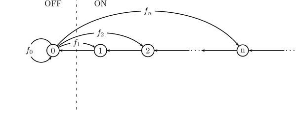
Figure 1: A topology used by models which generate LRD for particular choices of $f_{i}$.

A number of authors have used models of this form. Four models from the literature are discussed here.

Obviously this introduces a huge simplification into the modelling. The traffic model produced has uniform length packets and which can only have arrival times $n\Delta t$ where $n\in\mathbb{N}$ and $\Delta t$ is a characteristic of the system. Amongst those features not captured by such a model are

• The distribution of packet lengths shown by real life systems.

• The seasonality shown by real life systems (daily and weekly cycles).

• System behaviour arising from TCP feedback mechanisms.

• Usually packets are not constrained to arrive within some multiple of $\Delta t$.

Set against this, there is the analytical simplicity of such models. By investigating toy models where the behaviour can be understood it may be possible to gain an insight which is not possible in more complex models which capture more realistic features of the behaviour of network traffic.

2 Traffic generation models considered

Four models have been found in the literature of which two use the same topology but different parameters. In order to simplify the explanations given in this paper, the models will be described using the same notation even where this will differ from the notation given by the authors in the papers cited. While the Wang model was not actually suggested as a model for internet traffic, it is included here as it is the oldest model the author has found in the literature which associates on/off MMP with LRD.

The notation used is:

• ${\mathbf{P}}$ — the transition matrix of the underlying MC.

• $f_{k}$ — the transition probability to some state $k$ (in the models discussed it will usually be obvious where the transition was from).

• $\pi_{k}$ — the equilibrium distribution of some state $k$.

• $\mu$ — the mean number of packets generated per iteration ($\mathrm{E}\left[Y_{t}\right])$.

• $\alpha$ — a parameter giving the degree of LRD and related to the Hurst parameter $H$ by $H=(2-\alpha)/2$.

The physical interpretation of these parameters is important to understand. The interpretation of $f_{k}$ and $\pi_{k}$ depends on the topology of the model. For example, in the topology of the Wang or the Clegg/Dodson model then $f_{k}$ is the probability that a zero will be followed by exactly $k$ ones. The probability $\pi_{0}$ is the probability that (at equilibrium) the series will have the value zero — hence $\mu=1-\pi_{0}$ is the mean number of arrivals per unit time for the model. Similar interpretations can be made for the Arrowsmith/Barenco model.

The value of $\mu$ is critically important since it controls the amount of traffic the model will produce. The parameter $\alpha$ (not relevant for the PSST) which relates to the Hurst parameter also has important effects for queuing.

2.1 Wang model

The Wang model [19] grew out of the problems associated with calculating the invariant density of certain non-linear maps. In particular, it arises from a piecewise linearisation of the Manneville-Pomeau map [15] which is itself used in internet traffic modelling [8]. The topology of the MC is given in Figure 1 and therefore the transition matrix is

$${\mathbf{P}}=\left[\begin{array}[]{cccccc}f_{0}&f_{1}&f_{2}&\dots&f_{n}&\dots\\ 1&0&0&\dots&0&\dots\\ 0&1&0&\dots&0&\dots\\ 0&0&1&\dots&0&\dots\\ \vdots&\vdots&\vdots&\ddots&\vdots&\ddots\end{array}\right]$$ (4)

The finite version of this matrix is sometimes known as a companion matrix. The MC can be shown to be ergodic if $f_{0}>0$, if the sum $\sum_{i=0}^{\infty}if_{i}$ converges and if, for all $m\in\mathbb{N}$ there is $n>m:f_{n}>0$. For the Wang model, the transition probabilities are given by

$$f_{k}=\begin{cases}\frac{a}{k^{\alpha+1}}-\frac{a}{(k+1)^{\alpha+1}}&k\in\mathbb{N}\\ 1-a&k=0,\end{cases}$$

where $a\in(0,1)$ and $\alpha>0$ are parameters of the model. It has been shown [19] that if $\alpha\in(0,1)$ then the process will have LRD with

$$\rho(k)\sim k^{-\alpha}.$$

The mean $\mu$ is given for this topology (assuming the conditions for ergodicity are met) by

$$\mu=1-\pi_{0}=1-\left[1+\sum_{k=1}^{\infty}kf_{k}\right]^{-1},$$ (5)

where the expression in brackets comes from the mean first return time time for state 0. For the other states it can be easily shown that

$$\pi_{k}=\pi_{0}\sum_{j=k}^{\infty}f_{j}.$$

Substituting into (5) for the specific values this becomes

$$\mu=1-\left[1+\sum_{k=1}^{\infty}\frac{a}{k^{(\alpha+1)}}\right]^{-1}=1-\left[1+a\zeta(\alpha+1)\right]^{-1},$$ (6)

where $\zeta(\alpha+1)$ is the Riemann zeta function. While this model allows the Hurst parameter to be set, there is no closed form for the mean, though, given a value for $\alpha$ one could estimate the correct value for $a$ by an iterative procedure. It is easy to get expressions for the other equilibrium densities

$$\pi_{k}=\frac{(1-a)\pi_{0}}{1-\left[k/(k+1)\right]^{(\alpha+1)}}\qquad k\in\mathbb{N}.$$

This model has the advantage that the LRD has been shown analytically and can be set with a single parameter — choice of $\alpha$ determines the Hurst parameter of the simulated traffic. Computational modelling is relatively easy. There is no closed form for the equilibrium density of any of the states but the calculation is not difficult. There is no closed form solution for the value of $a$ corresponding to a particular mean once $\alpha$ has been set, however, such a value can be approximated using (6) rearranged to

$$a=\frac{\mu}{1-\mu}\zeta(\alpha+1)^{-1}.$$

2.2 The Pseudo-Self-Similar Traffic (PSST) model

The PSST model [17] was introduced to capture the LRD in packet traffic (they use the phrase self-similarity). In fact the model suggested is a finite model which would not generate self-similarity but the authors hope it would approximate it. The model is further investigated in [10] and criticised as providing unrealistic estimates for queuing performance. The topology of the PSST model is shown in Figure 2.

Figure 2: The topology of the PSST model.

The transition matrix for the model truncated after $n$ states (numbered $0$ to $n-1$) is given by.

$${\mathbf{P}}_{n}=\left[\begin{array}[]{ccccc}\Sigma_{0}&\frac{1}{a}&\frac{1}{a^{2}}&\dots&\frac{1}{a^{n-1}}\\ \frac{q}{a}&\Sigma_{1}&0&\dots&0\\ \left(\frac{q}{a}\right)^{2}&0&\Sigma_{2}&\dots&\\ \vdots&\vdots&\vdots&\ddots&\vdots\\ \left(\frac{q}{a}\right)^{n-1}&0&0&\dots&\Sigma_{n-1}\end{array}\right],$$

where

$$\Sigma_{0}=1-(1/a)-(1/a^{2})-\dots-(1/a^{n-1})$$

and $\Sigma_{i}=1-(q/a)^{i}$ for $i=1,\dots,n-1$. Note that for this to be a valid ergodic MC $a-a^{-(n-1)}>2$ and $a>q>1$. In the original model

$$Y_{t}=\begin{cases}1&X_{t}=0,\\ 0&\text{ otherwise },\end{cases}$$

This is a slightly strange choice because such a model would produce runs of packets which have a length which decays exponentially and runs of inter-packet gaps which are heavy-tailed. In this paper, this model will be referred to as PSST(a) and PSST(b) is the same model with on and off reversed (that is $Y_{t}=1$ if $X_{t}\neq 0$).

Previous references have used a truncated finite version of this model. However, there seems no particular reason to use this approximation and here the infinite model will be used. For $\Sigma_{0}$ the sum becomes

$$\Sigma_{0}=1-\frac{1-(1/a)^{n-1}}{a-1}$$

which for the infinite chain reduces to $\Sigma_{0}=a/(a-1)$.

For PSST(a) model the mean is given by

$$\mu_{a}=\pi_{0}=\frac{q^{n}-q^{n-1}}{q^{n}-1},$$

which in the infinite model becomes

$$\mu_{a}=\frac{q-1}{q}.$$

For the PSST(b) model the mean is given by $\mu_{b}=1-\mu_{a}=1/q$. This can be rearranged to $q=1/(1-\mu_{a})$ or $q=1/\mu_{b}$. The equilibrium probabilities of the states are given by

$$\pi_{k}=\frac{\pi_{0}}{q^{k}}.$$

However, there is no obvious interpretation of the $a$ parameter which, in some way, in combination with the ratio $q/a$, controls the long term decay of the model. Lower values of $q/a$ will lead to longer sojourn times in higher numbered states as $q/a$ becomes smaller. So it might be expected that lower values of $q/a$ would lead to higher correlations over large lags. The long-term behaviour of the model is discussed in section 2.5.

2.3 Arrowsmith/Barenco model

This model [2, 3] was introduced to capture the LRD seen in packet traffic and as a development of the Wang model. The topology is shown in Figure 3.

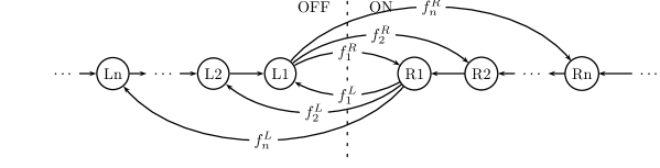
Figure 3: The topology of the Arrowsmith/Barenco model.

The expected sojourn time on the left hand side of the model $S_{L}$ is given by

$$S_{L}=\sum_{k=1}^{\infty}kf_{k}^{L},$$

and a similar expression can be given for the sojourn time on the right hand side $S_{R}$. This gives the expected number of packets per iteration as

$$\mu=\frac{S_{R}}{S_{R}+S_{L}}.$$

Because the model is a double-sided version of the Wang model then the decay of consecutive runs of zeros and ones can be individually controlled. An important result with this topology is [3, Theorem 4].

Theorem 1

Let

$$f_{k}^{L} \sim K_{L}k^{-\alpha_{L}+1}$$

$$f_{k}^{R} \sim K_{R}k^{-\alpha_{R}+1}$$

where $\alpha_{L},\alpha_{R}>0$ and $K_{L},K_{R}>0$ are all constants (here we will restrict $\alpha_{L},\alpha_{R}$ to $(0,1)$. Then

$$\rho(k)\sim Kk^{\beta},$$

where $\beta=\min(\alpha_{L},\alpha_{R})$ and $K$ is given by

$$K=\begin{cases}\frac{K_{R}(1-\mu)}{S(\alpha_{R}-1)\mu}&\alpha_{R}<\alpha_{L}\\ \frac{K_{L}\mu}{S(\alpha_{L}-1)(1-\mu)}&\alpha_{L}<\alpha_{R}\\ \frac{K_{R}(1-\mu)K_{L}\mu}{\mu(1-\mu)S(\alpha_{L}-1)}&\alpha_{L}=\alpha_{R},\end{cases}$$

where $S=S_{L}+S_{R}$.

In fact, no specific form for the values of $f_{k}$ are given in [3] and a variety of methods for choosing parameters for this model are given in [2].

2.4 Clegg/Dodson model

The Clegg/Dodson model [7] uses the same topology as the Wang model but different transition probabilities. The model has two parameters $\pi_{0}\in(0,1)$ which is related to the mean by $\pi_{0}=1-\mu$ and $\alpha\in(0,1)$ which determines the Hurst parameter. These are used to give the transition probabilities

$$f_{k}=\frac{1-\pi_{0}}{\pi_{0}}\left[k^{-\alpha}-2(k+1)^{-\alpha}+(k+2)^{-\alpha}\right],$$ (7)

for $k>0$ and for $k=0$,

$$f_{0}=1-\frac{1-\pi_{0}}{\pi_{0}}\left[1-2^{-\alpha}\right].$$ (8)

From these it can be shown that the model has equilibrium probabilities given by

$$\pi_{k}=(1-\pi_{0})[k^{-\alpha}-(k+1)^{-\alpha}]\qquad k>0.$$ (9)

which gives the sum

$$\sum_{i=k}^{\infty}\pi_{i}=(1-\pi_{0})k^{-\alpha}\qquad k>0.$$ (10)

This can be interpreted as the probability of a randomly chosen $Y_{t}$ being one and being followed by at least $k-1$ ones.

The model is only valid with $\alpha,\pi_{0}\in(0,1)$ if,

$$\pi_{0}>\frac{2^{\alpha}-1}{2^{\alpha+1}-1}.$$ (11)

If this condition is not met the model does not form a valid Markov chain. This rules out combinations with high Hurst parameter and high occupancy, near one (fortunately, these are unrealistic parameter sets for most networks).

It can be proved that the time series $Y_{t}$ generated by this model exhibits LRD with the Hurst parameter $H=1-\alpha/2$.

2.5 Long-term behaviour of the PSST model

It has been speculated but not shown that the PSST model generates traffic which exhibits long-range dependence. Further, the traffic from the PSST model has been analysed by measuring its Hurst parameter. However, there may be some reason to question this method. Consider $R_{0}$ the first return time to the zero state of the model. From the transition matrix it can be seen that,

$$\mathbb{P}\left[R_{0}>k\right]=\sum_{i=1}^{n}\frac{1}{a^{i}}(\Sigma_{i})^{k}.$$ (12)

Since $\Sigma_{i}\in(0,1)$, for any finite $n$ then as $k\rightarrow\infty$ this will fall off faster than some $x^{k}$ with $x\in(0,1)$ and therefore, this distribution cannot be heavy tailed. Only the infinite model can exhibit heavy tails in the return times to zero and hence the sojourn time of zeros in the PSST or ones in the PSST(b) model.

It can be simply shown that the infinite model does have heavy tails in the return time to zero. Recall that

$$\Sigma_{i}=1-(q/a)^{i},$$

and since $q/a<1$ then as $i\rightarrow\infty$ values of $\Sigma_{i}$ can be found arbitrarily close to one. To show that a distribution has a heavy tail we must prove condition (2) holds for all $\varepsilon>0$. For a given $\varepsilon>0$ there must be some $N:\Sigma_{N}>e^{-\varepsilon/2}$ ($N$ is a function of $\varepsilon$ and gets larger as $\varepsilon\rightarrow 0$). Taking just the term for $i=N$ in (12) gives

$$\mathbb{P}\left[R_{0}>k\right]>\frac{1}{a^{N}}(e^{-\varepsilon/2})^{k},$$ (13)

and therefore, the condition for the distribution of $R_{0}$ being heavy tailed is a condition on $\mathbb{P}\left[R_{0}>k\right]e^{\varepsilon}$ and a lower bound is given by

$$\mathbb{P}\left[R_{0}>k\right]e^{\varepsilon k}>\frac{1}{a^{N}}e^{-\varepsilon k/2}e^{\varepsilon k}=\frac{1}{a^{N}}e^{\varepsilon k/2}.$$

and for a fixed $\varepsilon>0$ and $N$ (which is a function of $\varepsilon$) this will become infinite as $k\rightarrow\infty$. This shows that for the infinite PSST the length of the OFF period has a heavy-tailed sojourn time (or the ON period for the PSST(b) model). However, the form of the asymptotic fall-off may not be the often-assumed form of (3). This would mean that theorem from [9] could not be applied and the LRD of the model could not be assumed.

The expression can be further expanded to give

$$\mathbb{P}\left[R_{0}>k\right] =\sum_{i=1}^{n}\sum_{j=0}^{k}\binom{k}{j}(-1)^{j}\left(\frac{q^{j}}{a^{j+1}}\right)^{i}$$

$$=\sum_{j=0}^{k}\binom{k}{j}\frac{(-q)^{j}(1-q^{jn}/a^{(j+1)n})}{(a^{j+1}-q^{j})}.$$

As $n\rightarrow\infty$ then $q^{jn}/a^{(j+1)n}\rightarrow 0$ and this becomes

$$\mathbb{P}\left[R_{0}>k\right]=\sum_{j=0}^{k}\binom{k}{j}\frac{(-1)^{j}}{a(a/q)^{j}-1}.$$ (14)

For $k$ odd the series can also be written as

$$\mathbb{P}\left[R_{0}>k\right] =$$

$$\sum_{j=0}^{(k-1)/2}\binom{k}{2j} \left[\frac{1}{a(a/q)^{2j}-1}-\frac{1}{a(a/q)^{(k-2j)}-1}\right].$$

While these expression are in a closed form they are not particularly convenient to work with computationally. The binomial coefficient becomes large for large $k$ as does the value of $(a/q)^{j}$ for large $j$ this makes the two expressions above hard to work with numerically and an arbitrary precision arithmetic library must be used to investigate large values of $k$.

Figure 4: Plot of $\mathbb{P}\left[R_{0}>k\right]$ versus $k$ for PSST model.

Figure 4 shows three different plots for (14) which all produce the same mean traffic (controlled by the $q$ parameter) but vary the $q/a$ ratio which controls the dependence. If the system has a power-law sojourn time then the log-log plot would tend to a straight-line as $k\rightarrow\infty$. However, as can be seen, this is not the case for two of the three lines here and for the range of $k$ plotted (although arguably might be the case for the $q/a=1/2$ line). These plots look at sojourn times of up to 1000. It may be that the plot would become linear. However, the case where $k=1000$ is the case where 1000 or more consecutive zeros (or ones in the PSST(b) model) appear and must be at the limits of what would be expected in even exceptionally long computational runs. In other words, this is the region of the model which computational runs will “see”.

In short, while the PSST model has a heavy-tail distribution in the sojourn time of the off state, it does not appear to have the expected power-law fall off. The author knows of no theorem which would prove the LRD or otherwise of the generated time-series. Even if the time-series generated did exhibit LRD it could be expected that it is the case that the LRD would appear in the summation of the autocorrelation of Definition 1 but not necessarily with the power-law fall of of (1). If this were the case then the model would not have a well-defined Hurst parameter. Measurements of the Hurst parameter on traffic produced by the PSST model vary greatly depending on the estimator used. This is discussed in section 3.4 and does not seem to have been noted by other investigators.

2.6 Computer implementation

These MMP described are relatively simple and fast to implement. For this paper, they have been implemented in the computer language python. By necessity a robust computational implementation of such routines must deal with very small probabilities. The phenomenon of LRD generated by such chains relies on the robust computation of the probability of some long run of ones or zeros. However, numerical rounding issues become important in practical implementations and a naive implementation would be subject to rounding errors. The rounding error problem is described here in relation to the Clegg/Dodson model. The full details are given in [7]. A robust implementation of any of these models is must overcome similar rounding problems and a similar approach can be used.

For example, a direct computation of $f_{k}$ for large $k$ in models using the topology 1 would lead to a very small number which may be hard to deal with computationally. Assume that the chain is in state zero at time $t$ ($X_{t}=0$). It is now necessary to find $\mathbb{P}\left[X_{t+1}=k\right]$ using the values of $f_{k}$. A naive implementation would choose the state to move to from the zero state by picking a single random number and comparing it with the probability distribution function. For low $k$ a direct computation of $\mathbb{P}\left[X_{t+1}=k\right]$ is well within the computational accuracy of the computer. For higher values then calculations of $\mathbb{P}\left[X_{t+1}\in[k,2k]|X_{t+1}\geq k\right]$ keep the numbers in a manageable range. This technique is employed for all four models here.

It should be noted that LRD is a difficult subject to work with computationally. Hurst parameters near unity ($\alpha$ near zero) cause great problems. Theoretically, the nearer one the Hurst parameter, the slower the sample mean will converge to the mean. To give a concrete example, $10^{6}$ iterations of the Clegg/Dodson model with $\mu=0.5$ and $\alpha=0.1$ ($H=0.95$) gives for the first three samples, $\overline{Y}=0.563$, $\overline{Y}=0.401$ and $\overline{Y}=0.426$. This does not indicate a problem with the computational model rather this slow convergence of the sample mean is inherent in the nature of LRD itself. Naturally, this has a critical importance to real experiments.

3 Experimental setup

The experiments performed in this paper are extremely simple. The input data for one simulation is a set of arrival times and packet lengths. These data may originate from real measurements or from the models described. The packets are then simulated as arriving at a queue of known output bandwidth. The properties of the queue and the output traffic are then measured. The experiment may then be repeated with a smaller output bandwidth to see how this affects the queue. Obviously as bandwidth decreases it would be expected that the mean queue length and queuing delays would increase but the exact behaviour depends upon the statistical nature of the traffic.

3.1 Data sets used

Two data sets are used for the simulation in this paper. In both cases, only the first 100,000 packets were investigated. The names and origin of the exact sources used are given here so that other researchers can make similar measurements.

CAIDA data: This data set is taken from a trace approximately an hour long. It is referred to as 20030424-000000-0-anon.pcap.gz and was captured on the 24th April 2003. It was captured on an OC48 link with a rate of 2.45 Gb/s. The average packet length was 493 bits. The data is freely available to researchers who fill in a request form. More information about this data can be found at:
www.caida.org/data/passive/.

Bellcore data: This much-studied data set is described in [12]. The data here is taken from an August 1989 measurement referred to as BC-pAug89.TL. The data was collected on an Ethernet link which connected a LAN to the outside world. Note that in this case the data did not record the true length of packets, only the length less the Ethernet header (which is variable). The average packet length recorded was 464 bits. Hence, the experiment in this paper is only using an approximation of the real data. The data is freely available for researchers. More information about this data can be found at:
ita.ee.lbl.gov/html/contrib/BC.html.

3.2 Queuing model, pre-processing and digitisation of real data

The queuing model used in this paper is extremely simple. The system has a given bandwidth $b$ (bits/sec). Items join the back of the queue. If a packet of length $L$ bits arrives at the queue then it will take a time $L/b$ to process. It is output from the queue at this time. Until this time the entire packet is considered to be part of the queue for purposes of calculating mean queue length (which can be calculated in terms of packets or bits).

A starting point for modelling is to establish a base case for comparisons. The real data simply consists of arrival times of packets and packet lengths. In order to attempt to match this data with real models, then a bandwidth $b$ was selected. This was chosen to create an occupancy near ten percent as this was thought to be a reasonable occupancy for a congested network. The Bellcore data was reported as being taken from a network with an occupancy of twenty percent at peak times. The CAIDA data almost certainly had an occupancy much lower than this since it is from a modern high-speed link. The actual figure chosen is not really important since the data are then to be queued through lower and lower bandwidths.

For the Bellcore data the baseline bandwidth was chosen as 1.96Mb/sec and for the CAIDA data 128Mb/sec this gave occupancies of and 0.094 and 0.098 respectively. Traffic with the recorded arrival times and packet lengths was then passed through this queue and the output times from this queue were taken as the base case to simulate. The data referred to as “raw” for the rest of this paper is the output of this queue with either the Bellcore or CAIDA packet lengths as an input.

The traffic generation models are all digitised in a way that the real data was not. The models all simply produce a string of ones and zeros corresponding to a packet or a gap. To convert these into packets and departure times a timescale $dt$ must be established and also a fixed packet length. The timescale $dt$ is the length of time between packets in a packet train or the length of one inter-packet gap. The packet length $l$ bits was chosen as the mean packet length of the real data (464 bits for the Bellcore data and 496 bits for the CAIDA). The timescale was then chosen related to the bandwidth as the time taken to transmit one packet of this length, that is $dt=l/b$.

Obviously this is a considerable simplification and it is therefore useful to investigate to what extent the real data would be altered if it were subject to this digitisation. Therefore a digitised version of the real data was produced where all the packets are of length $l$ and broadcast at fixed multiples of $dt$. This data is referred to as the digitised data. It was created simply by simulating a queue where the packets arrival times and packet lengths were taken from the real data. At every time $ndt:n\in\mathbb{N}$, if the queue contained $l$ or more bits then a packet of length $l$ was sent from the queue at this time. The data referred to as digitised throughout the rest of this paper is the results of this process with the input as the raw data and queued using the same bandwidth $b$ as the raw data.

Figure 5 shows the differences introduced by this digitisation process. These results are produced by queueing the Bellcore raw and digitised data in a queue with half the original bandwidth ($b$ is reduced from 1.96Mb/s to 0.98Mb/s). The top figure shows the distribution of the queue size in bits and the bottom figure shows the distribution of the queue in packets. As can be seen on the data in bits, the real data has a much more complex graph, simply because packets can have a variety of different lengths. Interestingly the raw data tends to have a higher queue length in terms of bits but lower in terms of packets. The reason for this is not known. The digitised data certainly shows differences to the raw data but the queuing performance is not greatly dissimilar. Further comparisons will be shown in the next section.

Figure 5: Plot of $\mathbb{P}\left[Q>q\right]$ with $q$ as the queue length in bits(top) and packets(bottom).

3.3 Models used to simulate data

Several on/off type models were tested against the real data to compare queuing performance. In addition to the MMP models already described two further models were used for comparison. The Poisson model is, perhaps, the simplest possible model. It either generates or does not generate a packet in every time period with a probability equal to the required mean. Note that strictly speaking this is a Bernoulli process but it is well approximated by a Poisson process. Fractional Gaussian Noise (FGN) is a well known process for generating data series with LRD. While it produces continuous traces it can be simply adapted to produce an on/off packet-gap model In practice, the PSST model was found to be extremely unstable for producing traffic with the low mean used. Successive realisations produced traces with extremely different means and the results from the model varied greatly from run to run — for example, with $q=1.104$ the model should produce a mean of 0.94. With $a=20$ three subsequent runs produced sample means of 0.11, 0.19 and 0.27. With $a=2$ (the lowest valid value for $a$) three subsequent runs produced sample means of 0.11, 0.11 and 0.07. In other words, the traffic level can increase by a huge amount between runs and it is impossible to get consistent results. For this reason, only the PSST(b) model results are presented here as this model produces a more consistent sample mean.

For the Arrowsmith/Barenco model a method was needed for estimating the $f_{i}^{L}$ and $f_{i}^{R}$ parameters. These parameters represent the probabilities of an inter-packet gap or packet train of length $i$ and this gives an obvious strategy for tuning them. The parameters are matched to the probability distribution of inter-packet gap and packet train lengths in the digitised data for each sample of traffic. This implies that the Arrowsmith/Barenco model will be producing traffic traces with the same distribution of packet train lengths and inter-packet gaps as the digitised data. Another method is described in [3] where the parameters of the model are tuned using genetic algorithms to match a given autocorrelation function. Many possible parameter selection strategies are available for this model and the comments in the rest of this paper should only be taken as reflective of the particular method of parameter selection. Note that this method for getting parameter settings means that the model does not replicate the Hurst parameter.

The Poisson model is a single parameter model, reflecting only the mean of the data. The Wang, Clegg/Dodson and FGN models are two parameter models which model the mean and the Hurst parameter. The PSST(b) model is a two parameter model which models the mean and a parameter related to correlations. The Arrowsmith/Barenco model as used here is a multi-parameter model which models the probability distribution of the lengths of packet trains and inter-packet gaps.

3.4 Calculation of Hurst parameter

Calculating the Hurst parameter of real data is not a simple matter. For a practical guide in the context of telecommunications and descriptions of the methods used in this paper see [6]. The methods used in this paper are the R/S estimator, Aggregated Variance, Periodogram, Wavelet analysis and the Local Whittle Estimator. Software using the statistics package R can be downloaded from:
http://www.richardclegg.org/lrdsources/software/. An excellent description of various methods and S-Plus code can be found at:
http://math.bu.edu/INDIVIDUAL/murad/home.html.

To calculate the Hurst parameter the data must first be converted into a time series. This can be done simply by counting the number of bytes processed if the data is split into sample times of a given period. The question is then which time period to choose. Too long a time period will give too small a sample size to work with (a ballpark figure is that several thousand time series points is a minimum). Too short a time period will give a time series which largely consists of zeros.

For the Bellcore date time periods of 0.1 seconds, 0.01 seconds and 0.001 seconds were tried. This resulted in 2521, 25208 and 252080 samples respectively. However, at the smallest sample size more than three quarters of the periods sampled have no packets at all.

Data	R/S	Agg. V.	Period.	Wav.	Loc. W.
Raw (0.1s)	0.757	0.509	0.657	0.689	0.855
Raw (0.01s)	0.75	0.751	0.845	0.769	0.828
Raw (0.001s)	0.798	0.765	0.79	0.809	0.736
Dig (0.1s)	0.756	0.509	0.657	0.689	0.856
Dig (0.01s)	0.748	0.751	0.845	0.769	0.828
Dig (0.001s)	0.787	0.765	0.788	0.81	0.79

Table 1: Hurst parameter estimates for Bellcore data.

Table 1 shows the results for the raw and digitised Bellcore data for the five estimators and three sampling rates as described above. The value of $H$ would normally be expected to lie between 0.5 (independent or short-range dependent data) and 1. As can be seen, at the slowest sampling rate (smallest sample size) there is little agreement between the estimators. It would be hard to justify giving more than one significant figure for $H$ given the low agreement between the estimators. When sampling at the two higher rates the estimators seem to agree on a Hurst parameter of around 0.8 (the exception being the Local Whittle estimator which gives 0.736 at the highest sampling rate for the raw data). The digitisation has made very little difference to the estimated Hurst parameter of the data in almost all cases.

The same procedure is performed for the CAIDA data. This data has a line speed and aggregation levels of 1000, 100 and 10 micro seconds were chosen which gives 3924, 39331 and 392301 samples respectively on the raw data (as with the Bellcore data, the raw and digitised data were in broad agreement and the digitised results are not presented here.) The results are shown in Table 2 and, again, while it is only appropriate to get $H$ to one decimal place the results broadly agree with a value of $H=0.6$. This is a low level of LRD (indeed it may be there is no LRD in this data) consistent with the rule of thumb that networks with lower utilisation often exhibit a lower level of long-range dependence.

Data	R/S	Agg. V.	Period.	Wav.	Loc. W.
Raw (1000us)	0.567	0.617	0.563	0.641	0.621
Raw (100us)	0.66	0.593	0.607	0.639	0.635
Raw (10us)	0.529	0.626	0.644	0.578	0.529

Table 2: Hurst parameter estimates for CAIDA data.

Data	R/S	Agg. V.	Period.	Wav.	Loc. W.
FGN (0.1s)	0.76	0.713	0.85	0.874	0.84
FGN (0.01s)	0.754	0.779	0.798	0.763	0.793
FGN (0.001s)	0.652	0.781	0.786	0.724	0.605
Wang (0.1s)	0.634	0.426	0.381	0.502	0.68
Wang (0.01s)	0.603	0.563	0.653	0.675	0.853
Wang (0.001s)	0.608	0.747	0.802	0.851	0.898
PSST (0.1s)	0.553	0.481	0.451	0.589	0.629
PSST (0.01s)	0.796	0.582	0.617	0.693	0.972
PSST (0.001s)	0.705	0.709	0.868	1.07	1.35
Arr./Bar. (0.1s)	0.553	0.504	0.458	0.448	0.549
Arr./Bar. (0.01s)	0.634	0.52	0.538	0.597	0.619
Arr./Bar. (0.001s)	0.582	0.59	0.605	0.612	0.703

Table 3: Hurst parameter estimates for 100,000 packet realisations of simulated data.

Hurst parameter estimates were also made for the simulated data. The Wang model and FGN models were uses to simulate the Bellcore data using a theoretical Hurst parameter $H=0.8$ and the same theoretical mean as the Bellcore data. The models are run to produce 100,000 packets and aggregated as before to produce Hurst parameter estimates. The PSST(b) model is also used with the same theoretical mean as the data and a=500.

Table 3 shows the Hurst parameter estimates for models attempting to simulate the parameters of the Bellcore data. As can be seen, despite the theoretically sound nature of the FGN and Wang method, the estimators are not actually in very good agreement with the theory. This is not an unfamiliar situation to researchers studying the field of LRD estimation. From the table, the FGN Hurst parameter is estimated reasonably at an aggregation level of 0.1 and 0.01 seconds and rather underestimated at an aggregation level of 0.001 seconds. The Wang model also produces a variety of estimates for $H$ with the R/S estimator being particularly bad and the estimates at an aggregation of 0.1 seconds being so low that a researcher might conclude there was no LRD present.

The PSST model is spectacularly inconsistent. Considering the $H$ parameter is usually expected to be in the range $H=(1/2,1)$ for LRD and $H=1/2$ for no LRD, the estimates for the model vary across the entire available range and outside it. The estimates also change completely depending on the aggregation level considered. This is consistent with the hypothesis that if the PSST model does indeed produce traffic with LRD it does so in such a way that the traffic has no Hurst parameter.

Note that the method for choosing parameters for the Arrowsmith/Barenco model does not reproduce the Hurst parameter and this can be seen. While the Bellcore data had a measured Hurst parameter around $H=0.8$ the Arrowsmith/Barenco model tuned to have the same distribution of packet train lengths and inter-packet gaps has a measured Hurst parameter around $H=0.6$.

If the sample trace is longer then better estimates of the Hurst parameter are obtained for all models apart from the PSST(b) model. Table 4 shows a typical set of results for 1,000,000 packet realisations. The Wang model is producing data with a Hurst parameter of 0.8 and, while all of the estimators but the R/S are overestimating, they are not doing so greatly and are largely consistent with scales. The Clegg/Dodson model and FGN model also behave as expected. The PSST(b) model continues to produce widely differing estimates for $H$ which vary with aggregation scale. The PSST model shows similar behaviour.

Note that [10] reports that the PSST model was tuned to replicate the value of $H$ for real data. It is possible that the authors only had a single $H$ estimator available and thus did not notice these discrepancies. In this paper the $a$ parameter for the PSST(b) model was chosen simply to be “large” for the high Hurst case and smaller for the low Hurst case. No more scientific fitting procedure was available for the model.

Data	R/S	Agg. V.	Period.	Wav.	Loc. W.
Wang (0.01s)	0.612	0.885	0.858	0.842	0.875
Wang (0.001s)	0.724	0.859	0.840	0.852	0.905
PSST(b) (0.01s)	0.604	0.668	0.682	0.761	0.971
PSST(b) (0.001s)	0.846	0.74	0.88	1.076	1.349

Table 4: Hurst parameter estimates for 1,000,000 packet realisations of simulated data.

4 Results

The experiments performed are all of the same nature. The input to an experiment is data either from a real data source (raw or digitised) or from one of the models with its parameters tuned to match that of the digitised data. The input data is then sent through a queue with a given bandwidth $b$. The queuing performance of the model is then measured. While many performance measures could be considered, results are only given here in terms of the expected queue size $\mathrm{E}\left[q\right]$. The experiment is then repeated with a smaller value of $b$ until experiments have been performed with occupancies ranging from 0.1 to 0.6 (the latter representing a network with an extremely high degree of congestion).

4.1 Bellcore data

All models were run to produce traces 252 seconds long (the length of the original trace) with packets of length 464 bits. The model parameters were all chosen to replicated the mean of the original data. For the Clegg/Dodson, FGN and Wang models the second model parameter was chosen to replicate the Hurst parameter $H=0.8$ (although parameters higher and lower were tried). For the PSST(b) model $q=10.4$ was chosen to capture the correct mean. Various values of $a$ were tried but, as has been mentioned, tuning the model to replicate the Hurst parameter was impossible. The results presented here used $a=500$ which was considered to provide quite a high level of correlations. The model was tested with various other $a$ values with little more success than that reported here. The Arrowsmith/Barenco model was tuned to replicate the distribution of the packet-train lengths and inter-packet gaps of the digitised data as previously described.

Figure 6: Comparison of Poisson model versus real traffic for Bellcore data.

Figure 7: Comparison of FGN model versus real traffic for Bellcore data.

Figure 8: Comparison of Wang (model versus real traffic for Bellcore data.

Figure 6 shows comparisons of the Poisson model with the real data (both raw and digitised). Note that the $y$ axis is a logscale on this and all following figures. The theory line for the Poisson model is provided by the Pollaczek–Khinchin formula (with the discrepancy being accounted for by the fact that the model is, strictly speaking, Bernoulli not Poisson). As can be seen, and as would be expected, the Poisson model hugely underestimates the level of queuing in the network. This result is as would be expected from the literature.

Figure 7 shows a comparison of the FGN model versus real traffic. Several realisations of FGN are tried. Three realisations have $H=0.8$, one has $H=0.85$ and one has $H=0.75$. As can be seen the model produces more or less the same queuing performance with the same mean and Hurst parameter and a higher Hurst parameter produces larger queues. This is as would be expected from the literature. However, both are under predicting the queuing of the real data.

Figure 8 shows a comparison of the Wang model versus real traffic. Again several realisations of the Wang model are used. Again the model is producing similar queuing performance for the three models with the same mean and Hurst parameter. Note that the model with a Hurst parameter of $H=0.85$ has higher occupancy simply because this realisation happens to have produced data with a sample mean greater than the actual mean of the process. This is a common problem with LRD processes with high $H$ where the sample mean can converge slowly to the actual mean. The most striking thing though is that again all the models have failed to capture the queuing performance of the real data. In this case the models have greatly over estimated the amount of queuing which will occur.

Figure 9 shows a comparison with all of the models used against the real traffic trace. What is most striking about this is that none of the models are even close to replicating the real data. The raw and digitised data are relatively close together. The Clegg/Dodson and Wang models appear to be similar in performance (perhaps unsurprisingly since they have the same topology but different parameters). Both of these models overestimate queuing. The PSST model produces a higher queue level than these two models and is, obviously an overestimate of the queuing of the real data. The Poisson model, as has been mentioned, is an underestimate of the real queuing performance as is the FGN model. Interestingly, for low occupancies, the Poisson model is actually giving higher queues than the FGN model even though this model was motivated by addressing the underestimation of queuing in the Poisson model. The Arrowsmith/Barenco model is, perhaps, the closest model to the real data but this particular method must still be regarded as having failed to successfully model the queuing performance of the Bellcore data. Also the model used is a multi-parameter model as opposed to a one or two parameter model like the others and hence would be expected to be a much closer match.

A subtle but important difference in the figure is that in the regions with higher occupancy (the right hand side of the graph) the slope of the lines is very different. With the exception of the FGN model, in this region the models appear to have parallel lines on this figure but these lines have a very different gradient to the plots for the raw and digitised data. In other words, not only the level of congestion is different but the way the data responds to an increase in congestion is fundamentally different.

Figure 9: Comparison of all models on Bellcore data looking at the expected queue length.

Another way of comparing the models is to look at the probability of given queue lengths. Here, a similar graph to Figure 9 is plotted with the $y$ axis as the probability of the queue being equal to or greater than a given length. Figure 10 shows the probability of the queue equalling or exceeding five (top) or twenty (bottom). As can be seen, again none of the models are doing a good job of approximating these probabilities. The raw and digitised data remain similar to each other. At low occupancies the Poisson, FGN and Arrowsmith/Barenco models seem to be the best approximations and at high occupancies the Clegg/Dodson and Wang models seem to be closer. None of the models prove accurate over the whole range. The models prove poor approximations over the whole range of occupancies considered, no matter what the queue length chosen.

Figure 10: Comparison of all models on Bellcore data looking at the probability that the queue is five or greater (top) or twenty or greater (bottom).

4.2 CAIDA data

All models were run to produce traces 4.02 seconds long (the length of the original trace) with packets of length 496 bits. Again the model parameters were all chosen to replicated the mean of the original data and, for the Clegg/Dodson, FGN and Wang models the Hurst parameter $H=0.6$. For the PSST(b) model $q=10.2$ was chosen to capture the correct mean and $a=30$ was used to give a low level of correlation. The Arrowsmith/Barenco model was tuned as for the Bellcore data.

Figure 11 shows a comparison of all the models versus the real and digitised data. In most ways the results are similar to the results of modelling the Bellcore data. Again the Clegg/Dodson and Wang models are similar but provide an overestimate of the level of queuing. Again the FGN and Poisson models provide an underestimate of the queuing in this case with the FGN model giving a lower estimate of queuing than the Poisson model. In this case, however, the Arrowsmith/Barenco model has provided a very good estimate of the queuing lying somewhere between the raw and digitised data. The PSST model has provided a better approximation although it is still an over estimate. Again, however, the same feature can be seen as with the Bellcore data, in the high occupancy region (at the right hand side of the graph) the artificial models (with the exception of the FGN) seem to have run parallel (they appear to have approximately the same gradient). However, the real data appears to have a steeper gradient than any of the models in this region.

Figure 11: Comparison of all models on CAIDA data.

Again, the experiments can be repeated looking at the probabilities of the queue exceeding a given length. As for the Bellcore data, the probability of the queue length exceeding certain levels are plotted. Figure 12 shows the probability that the queue equals or exceeds five (top) or twenty (bottom). In the case of the queue exceeding five, the Arrowsmith/Barenco model gives an excellent approximation for most of the range of the experiment. Indeed it lies between the raw and digitised lines. The Wang and Clegg/Dodson (and possibly even PSST) models could also be seen to be acceptably close. For the more extreme event assessed by the probability that the queue exceeds twenty, the Wang and Clegg/Dodson models are clearly overstating the probability of these extreme queues. The PSST(b) model is a relatively good approximation of the real data. All other models seem to be underpredicting the likelihood of large queues at high occupancies.

Figure 12: Comparison of all models on CAIDA data looking at the probability that the queue is five or greater (top) or twenty or greater (bottom).

4.3 Later sections of data

As has been seen, it is a difficult task to replicate the queuing performance of a sample of 100,000 packets of real data. It might then be asked, if this sample could, in principle be replicated with one hundred percent accuracy then would this modelling be appropriate for subsequent data samples from this data. Figure 13(top) shows the second, third, fourth and fifth samples of 100,000 packets of the Bellcore data queued by the same process (raw data). As can be seen the queuing performance of the data varies greatly between these samples. Note that each point plotted corresponds to a different bandwidth for queuing but the data differs also in the mean packets transmitted and hence the occupancy differs between samples. However, the differences are far from being differences purely due to the time over which the packets transmitted. Consider, for example the first 100,000 packets compared to the third 100,000. The third 100,000 packets have a lower occupancy (that means they took longer to transmit and are sampled from a period of time where, on average, packets were being sent at a lower rate) but a higher queue.

Figure 13 (bottom) shows a similar plot for the CAIDA data. In this case, while the mean rate of data transmission still differs between samples, the queuing performance is broadly similar.

Figure 13: Comparison of subsequent sections of Bellcore data (top) and CAIDA data (bottom).

4.4 Discussion and criticism of results

The results presented here show an important weakness in a class of MMP models which have been used to emulate network traffic. Over all the data sets used, no models gave a good representation of the expected queue or queue overflow probabilities for the Bellcore data. It should be noted again that the model referred to as the Arrowsmith/Barenco model was just one method for choosing parameters for this model and this is not a general criticism of using this topology for modelling data. For the expected queue length, the Arrowsmith/Barenco model gave a good representation of the CAIDA data and the PSST(b) model gave a fair representation. In the case of the PSST(b) model there is no good way the author knows of picking one of the model’s parameters and it may be that this match is little more than coincidence. No models seemed able to predict the queue overflow probabilities of the CAIDA data for all queue lengths and all occupancies (although perhaps this would be demanding too much of such simple models).

The CAIDA data had a lower degree of long-range dependence. Also the CAIDA model had a more consistent performance between subsequent samples of 100,000 packets. It may be suspected that these two facts are related but it is hard to tell without further investigation.

One obvious criticism of the experiments performed here is that a real network would not behave like this under queuing. The TCP/IP protocol incorporates mechanisms which perform crude congestion control. In short, what is described here as the real data is not, in fact, how a real network would perform subject to the capacity constraints. This criticism is an important one and it is certainly true that a closed loop model incorporating this feedback would be a better representation of what actually happens when a real network becomes more congested. However, this said, good open loop models would greatly help the understanding of what factors in real network traffic impact on queuing performance. It would be much harder to understand how bandwidth impacted a closed loop system and it could be reasonably expected that changes to a network which were positive for an open loop system were also positive for a closed loop system (although this is by no means guaranteed).

Other models may be capable of producing a better model of the queuing performance of internet traffic. In [2] a method is described for tuning the parameters of the Arrowsmith/Barenco model to replicate the ACF of a traffic sample using genetic algorithms. Wavelets have been used not just for analysis of traffic traces (as in this paper) but also for simulating traffic [16] [1]. It is not clear, however, how an individual packet model could be generated from a time series produced using wavelet.

5 Conclusion

This paper presented a number of MMP models which produce on/off sequences. These models have all been suggested as potential models of telecommunications data (with the exception of the Wang model which arose in the field of Statistical Mechanics). In addition the FGN model was included since this is also a commonly suggested model for telecommunications data and the Poisson model was included as a baseline for comparisons. It is clear that in all cases the Poisson modelling was inappropriate and gave misleading queuing estimates.

While the Wang, Clegg/Dodson and FGN models captured the mean and Hurst parameter of the data, they did not accurately reflect the queuing performance of the system. Investigation of those models made it clear that, within those models, the Hurst parameter had a very important effect on queuing performance with a high Hurst parameter equating to worse queuing performance.

The PSST model proved hard to work with and the criticisms of this model by other authors seem justified [10]. However, this author is sceptical of the claim in [10] that the model can be fitted to provide a particular Hurst parameter. The PSST model does not seem to provide a traffic trace with a controllable Hurst parameter. In addition the original PSST model exhibits a remarkable degree of instability in its sample mean when the mean is set to produce a low level of traffic (a value of $q$ near 1). This said, the PSST(b) model was the only two parameter model to have any degree of success in modelling either data set.

The Arrowsmith/Barenco model as used in this paper did not model the Bellcore data well but was a very good model for the CAIDA data. It should be recalled that in this paper, a particular method for fitting the model parameters was used and the Arrowsmith/Barenco model is more general than the particular model used here. The model used in this paper is a multi-parameter model and would be expected to provide a better fit than one or two parameter models.

It is important to note that in the case of the high Hurst parameter Bellcore data, even if a model were found which accurately represented the queuing performance of the first 100,000 packets subsequent samples of 100,000 packets behaved very differently. On the other hand, for the CAIDA data which had a lower Hurst parameter, subsequent samples of the data performed more consistently.

In short, the problem of replicating the statistics of real traffic traces is a difficult one. The models tried in this paper all have their attractions in terms of computational or mathematical simplicity but none of them proved adequate to model the queuing performance of a traffic trace taken from a real network. If researchers are to truly understand what causes and can relieve queuing in telecommunications networks then an open loop model of this type would be an important starting point.

References

- [1] P. Abry, P. Flandrin, M. S. Taqqu, and D. Veitch. Self-similarity and long-range dependence through the wavelet lens. In P. Doukhan, G. Oppenheim, and M. S. Taqqu, editors, Theory and Applications of Long-Range Dependence, pages 526–556. Birkhäuser, 2003.
- [2] M. Barenco. Packet Traffic in Computer Networks. PhD thesis, School of Mathematical Sciences, Queen Mary, University of London, 2002.
- [3] M. Barenco and D.K. Arrowsmith. The autocorrelation of double intermittency maps and the simulation of computer packet traffic. Dynamical Systems, 19(1):61–74, 2004.
- [4] J. Beran. Statistics For Long-Memory Processes. Chapman and Hall, 1994.
-
[5]
R. G. Clegg.
Statistics of Dynamic Networks.
PhD thesis, Dept. of Math., Uni. of York., York., 2004.
Available online at:
www.richardclegg.org/pubs/thesis.pdf. -
[6]
R. G. Clegg.
A practical guide to measuring the Hurst parameter.
International Journal of Simulation: Systems, Science &
Technology, 7(2):3–14, 2006.
Available online at:
www.richardclegg.org/pubs/rgc_ijs.pdf. -
[7]
R. G. Clegg and M. M. Dodson.
A Markov based method for generating long-range dependence.
Phys. Rev. E, 72:026118, 2005.
Available online at:
www.richardclegg.org/pubs/rgcpre2004.pdf. - [8] A. Erramilli, R. P. Singh, and P. Pruthi. Chaotic maps as models of packet traffic, volume 1, pages 329–338. 1994.
- [9] D. Heath, S. Resnick, and G. Samorodnitsky. Heavy tails and long-range dependence in on/off processes and associated fluid models. Math. of Oper. Res., (1):145–165, 1998.
- [10] R. El Abdouni Khayari, R. Sadre, B. R. Haverkort, and A. Ost. The pseudo-self-similar traffic model:application and validation. Perform. Eval., 56:3–22, 2004.
- [11] W. E. Leland, M. S. Taqqu, W. Willinger, and D. V. Wilson. On the self-similar nature of Ethernet traffic. In D. P. Sidhu, editor, Proc. ACM SIGCOMM, pages 183–193, San Francisco, California, 1993.
- [12] W. E. Leland and D. V. Wilson. High time-resolution measurement and analysis of LAN traffic: Implications for LAN interconnection. Proc. IEEE INFOCOM, pages 1360–1366, 1991.
- [13] S. Li and C. Hwang. Queue response to input correlation functions: Discrete spectral analysis. IEEE/ACM Trans. on Networking, 1(5):522–533, October 1993.
- [14] A. L. Neidhardt and J. L. Wang. The concept of relevant time scales and its application to queuing analysis of self-similar traffic (or is Hurst naughty or nice?). In Proceedings of the 1998 ACM SIGMETRICS joint international conference on Measurement and Modeling of Computer Systems, pages 222–232, 1998.
- [15] Y. Pomeau and P. Manneville. Intermittent transition to turbulence in dissipative dynamical systems. Commun. Math. Phys., 74(2), 1980.
- [16] R. H. Riedi, M. S. Crouse, V. J. Ribeiro, and R. G. Baraniuk. A multifractal wavelet model with application to network traffic. IEEE Special Issue On Information Theory, 45(April):992–1018, 1999.
- [17] S. Robert and J.-Y. Le Boudec. New models for pseudo-self-similar traffic. Perform. Eval., 30:57–68, 1997.
- [18] Z. Sahinoglu and S. Tekinay. On multimedia networks: Self similar traffic and network performance. IEEE Communications Magazine, pages 48–52, January 1999.
- [19] X. J. Wang. Statistical physics of temporal intermittency. Phys. Rev. A, 40(11):6647–6661, 1989.
- [20] W. Willinger, V. Paxson, R. H. Riedi, and M. S. Taqqu. Long-range dependence and data network traffic. In P. Doukhan, G. Oppenheim, and M. S. Taqqu, editors, Theory And Applications Of Long-Range Dependence, pages 373–407. Birkhäuser, 2003.
- [21] W. Willinger, M. S. Taqqu, R. Sherman, and D. V. Wilson. Self-similarity through high-variability: statistical analysis of Ethernet LAN traffic at the source level. IEEE/ACM Trans. on Networking, 5(1):71–86, 1997.